On the Measurement of the Lense-Thirring effect using the nodes of the LAGEOS satellites, in reply to “On the reliability of the so-far performed tests for measuring the Lense -Thirring effect with the LAGEOS satellites” by L. Iorio

I. Ciufolini^a and E. Pavlis^b

^aDipartimento di Ingegneria dell’Innovazione, Università di Lecce, Via Monteroni, 73100 Lecce, Italy

^bJoint Center for Earth Systems Technology (JCET/UMBC), University of Maryland, Baltimore County, 1000 Hilltop Circle, Baltimore, Maryland, USA 21250

Abstract

In this paper, we provide a detailed description of our recent analysis and determination of the frame-dragging effect obtained using the nodes of the satellites LAGEOS and LAGEOS 2, in reply to the paper “On the reliability of the so-far performed tests for measuring the Lense Thirring effect with the LAGEOS satellites” by L. Iorio (doi: 10.1016/j.newast.2005.01.001). First, we discuss the impact of the $\dot{J}_{2n}$ uncertainties on our measurement and we show that the corresponding error is of the order of 1 $\%$ of frame-dragging only. We report the result of the orbital simulations and analyses obtained with and without $\dot{J}_{4}$ and a with $\dot{J}_{4}$ equal to its EIGEN-GRACE02S value plus 12 times its published error, i.e., a $\dot{J}_{4}$ equal to about 611 $\%$ of the value adopted in EIGEN-GRACE02S, that is $\dot{J}_{4}=6.11\times(-1.41\cdot 10^{-11})\simeq-8.61\cdot 10^{-11}$. In all these three cases, by also fitting the final combined residuals with a quadratic, we obtain the same value of the measured Lense-Thirring effect. This value differs by only 1 $\%$ with respect to our recent measurement of the Lense-Thirring effect. Therefore, the error due to the uncertainties in $\dot{J}_{2n}$ in our measurement of the gravitomagnetic effect can at most reach 1 $\%$, in complete agreement with our previously published error budget. Our total error budget in the measurement of frame-dragging is about $5\%$ of the Lense-Thirring effect, alternatively even by simply considering the published errors in the $\dot{J}_{2n}$ and their recent determinations we get a total error budget of the order of 10 $\%$, in complete agreement with our previously published error budget. Furthermore, we explicitly give the results and plot of a simulation clearly showing that the claim of Iorio’s paper that the $\dot{J}_{2n}$ uncertainty may contribute to up a 45 $\%$ error error in our measurement is clearly unsubstantiated. We then present a rigorous proof that any “imprint” or “memory” effect of the Lense-Thirring effect is completely negligible on the even zonal harmonics produced using the GRACE satellites only and used on the orbits of the LAGEOS satellites to measure the frame-dragging effect. In this paper we do not discuss the problem of the correlation of the Earth’s even zonal harmonics since it only refers to our previous, 1998, analysis with EGM96 and it will be the subject of a different paper; nevertheless, we stress that in the present analysis with EIGENGRACE02S the total error due to the static Earth gravity field has been calculated by pessimistically summing up the absolute values of the errors due to each Earth’s even zonal harmonic uncertainty, i.e., we have not used any covariance matrix to calculate the total error but we have just considered the worst possible contribution of each even zonal harmonic uncertainty to the total error budget. We also present and explain our past work on the technique of measuring the Lense-Thirring effect using the LAGEOS nodes and give its main references. Finally we discuss some other minor points and misunderstandings of the paper by Iorio, including some obvious mistakes contained both in this paper and in some other previous papers of Iorio. In conclusion, the criticisms in Iorio’s paper are completely unfounded and misdirected: the uncertainties arising from the possible variations of $\dot{J}_{2n}$ are fully accounted for in the error budget that we have published.

1 Error due to the $\dot{J}_{2n}$ in the 2004 measurement of the Lense-Thirring effect

In order to discuss the error analysis and the total error budget of our measurement of the Lense-Thirring effect (?), we first stress that in the data reduction of our recent measurement of the Lense-Thirring effect (?) we have used the value of $\dot{J}_{4}=-1.41\cdot 10^{-11}$, adopted by GFZ in the EIGEN-GRACE02S Earth gravity model (?), and we have fitted our combined residuals with a secular trend only plus a number of periodical terms. We can of course introduce $\dot{J}_{4}$ as a free parameter in our fit (see below). In this case, together with the measurement of the Lense-Thirring effect, we also measure the effect of the secular variations of $J_{2}$, $J_{4}$ and $J_{6}$ on the combination of the nodal longitudes of the LAGEOS satellites; this is described by a $\dot{J}_{4}^{Effective}$ (?) in our combination, which includes the effect of the secular variation of the higher even zonal harmonics. In (?) it is indeed reported an effective value of $\dot{J}_{4}^{Effective}\cong-1.5\cdot 10^{-11}$ for the combination of the LAGEOS satellites nodes, which is consistent with the EIGEN-GRACE02S model since, on our combination of the nodal longitudes of the LAGEOS satellites, it just represents a 6 $\%$ variation of the value given with EIGEN-GRACE02S and, however, it includes the effect of any higher $\dot{J}_{2n}$, with $2n\geq 4$; this value is also fully consistent with our published result of a Lense-Thirring drag equal to 99 $\%$ of the general relativity prediction with uncertainty of 5 $\%$ to 10 $\%$. It is easily seen, even by visual inspection, that our combined residuals would clearly display any such quadratic term. Indeed, in figure (1) we show the residuals obtained using the $\dot{J}_{4}$ value given with EIGEN-GRACE02S that should be compared with a simulation of the orbital residuals, shown in figure (5), obtained using in the data reduction a strongly unrealistic value of $\dot{J}_{4}$ corresponding to the value adopted in EIGEN-GRACE02S plus 12 times its published error and which produces a $\sim 45\%$ variation of the secular trend as claimed by the author of (?)! It is clear that only the first figure can be simply described by a linear dependence.

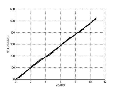
Figure 1: Fit of the residuals of the nodes of LAGEOS and LAGEOS II, using our combination and the Earth’s model EIGEN-GRACE02S, with a secular trend plus six periodical terms. The slope is $\mu\simeq 0.99$ (Ciufolini and Pavlis 2004).

In the EIGEN-GRACE02S model (?), obtained by the GRACE mission only, the Earth gravity field was measured during the period 2002-2003. Corrections due to $\dot{J}_{2}$ and $\dot{J}_{4}$ were then applied to this 2002-2003 measurement in order to obtain a gravity field model antecedent to 2002-2003. These values of $\dot{J}_{2}$ and $\dot{J}_{4}$, used by the GFZ team, are $\dot{J}_{2}=-2.6\cdot 10^{-11}$ and $\dot{J}_{4}=-1.41\cdot 10^{-11}$ and they were measured on the basis of completely independent 30-year observations before 2002.

Let us describe the result of the orbital analyses using the orbital estimator GEODYN with and without a contribution of $\dot{J}_{4}=-1.41\cdot 10^{-11}$, and the result of a simulation with a $\dot{J}_{4}$ equal to 611 $\%$ of the value given in EIGEN-GRACE02S, i.e. $\dot{J}_{4}\simeq-8.61\cdot 10^{-11}$.

First, we stress again that in the case of not applying the $\dot{J}_{4}$ EIGEN-GRACE02S correction to the orbital analysis, its effect can be clearly identified (but nevertheless completely fitted for, see below) even by visual inspection since it shows up as a hump in the combined residuals, whereas in our fit of (?) shown in Fig. 1 the absence of any such quadratic effect is obvious. Then, since the effect of the time variation $\dot{J}_{4}$ shows up as a quadratic effect in the cumulative nodal longitude of the LAGEOS satellites, the combined residuals of LAGEOS and LAGEOS 2 may be fitted with a quadratic curve, together with a straight line and with the main periodic terms. Thus, by fitting the raw residuals obtained without any $\dot{J}_{4}$ in a $test-analysis$, see Fig. 2, we measured a $\dot{J}_{4}^{Effective}\cong-1.5\cdot 10^{-11}$, which includes the effect of $\dot{J}_{6}$ and of higher even zonal harmonics on the combination of the LAGEOS nodes. On other hand, by fitting the combined residuals obtained with the EIGEN-GRACE02S correction of $\dot{J_{4}}=-1.41\cdot 10^{-11}$, we measured a $\delta\dot{J}_{4}^{Effective}$ of less than $-0.1\cdot 10^{-11}$, see Fig. 3, and this fitted difference is in complete agreement with the previous case. In all the cases of inclusion of an anomalous $\dot{J_{4}}$ in the data analysis, we obtained a measured value of $\mu\cong 0.98$, see Figures 3 and 4.

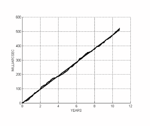
Figure 2: Fit of the residuals of the nodes of LAGEOS and LAGEOS II, using our combination and the Earth’s model EIGEN-GRACE02S, with a secular trend plus six periodical terms plus a quadratic. The residuals have been obtained without inclusion of any $\dot{J}_{4}$ value in the orbital analysis, i.e., using $\dot{J}_{4}=0$. The Lense-Thirring slope is $\mu\simeq 0.98$.

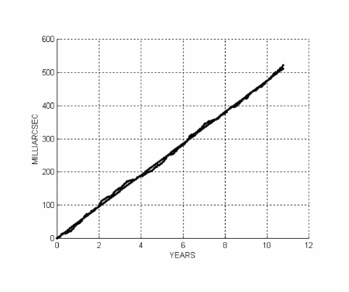
Figure 3: Fit of the residuals of the nodes of LAGEOS and LAGEOS II, using our combination and the Earth’s model EIGEN-GRACE02S, with a secular trend plus six periodical terms plus a quadratic. The residuals have been obtained using the $\dot{J}_{4}$ value given in the EIGEN-GRACE02S model. The Lense-Thirring slope is $\mu\simeq 0.98$.

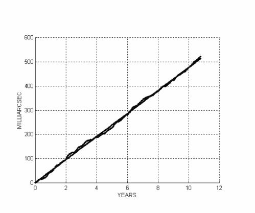
Figure 4: Fit of the residuals of the nodes of LAGEOS and LAGEOS II, using our combination and the Earth’s model EIGEN-GRACE02S, with a secular trend plus six periodical terms plus a quadratic. The residuals have been obtained using a $\dot{J}_{4}$ value equal to 611 $\%$ of the $\dot{J}_{4}$ value given in the EIGEN-GRACE02S model. The Lense-Thirring slope is $\mu\simeq 0.98$.

Therefore, the small value of the unmodelled quadratic effects in our nodal combination due to the unmodelled $\dot{J}_{2n}$ effects (with $2n\geq 4$) corresponds to a change in the measured value of the Lense-Thirring effect of about 1 $\%$ only. As a consistency test, using the value $\dot{J}_{4}^{Effective}=-1.5\cdot 10^{-11}$, obtained from fitting the combined residuals (which is only about 6 $\%$ larger than the value $\dot{J}_{4}=-1.41\cdot 10^{-11}$ given in the EIGEN-GRACE02S model), we have again generated the residuals and fit these with a straight line only plus the main periodic terms. It turned out that the change of the measured value of frame-dragging was about 1 $\%$ only with respect to the case of using $\dot{J}_{4}-1.41\cdot 10^{-11}$ and fitting the residuals with a straight line plus the main periodic terms (?), i.e., this test resulted in a measured value of $\mu\cong 0.98$. The result of this test agrees with the case of fitting the combined orbital residuals with a straight line plus a quadratic curve, indeed in all cases we got $\mu\cong 0.98$, see Figures 2, 3 and 4. As a third case, using in the data reduction a highly unrealistic value of $\dot{J}_{4}$ equal to the value adopted in EIGEN-GRACE02S plus 12 times its published error, i.e., a $\dot{J}_{4}$ equal to about 611 $\%$ of the value given in EIGEN-GRACE02S, that is $\dot{J}_{4}=6.11\times(-1.41\cdot 10^{-11})\simeq-8.61\cdot 10^{-11}$, by fitting the residuals with a straight line plus the main periodic terms plus a parabola, we again obtained the same measured value of frame-dragging, i.e., $\mu\cong 0.98$, see Fig. 4. Therefore, also in this case the measured value of frame-dragging differs by about 1 $\%$ only with respect to the case of using $\dot{J}_{4}=-1.41\cdot 10^{-11}$ without fitting a quadratic curve, i.e., the result reported in (?) and in Fig. (1).

These analyses clearly show that even in the cases of - 100 $\%$ and + 511 $\%$ variations between the value of $\dot{J}_{4}$ of Mother Nature and the value used in the orbital estimation of (?), it is possible to fit for the $\dot{J}_{4}^{Effective}$ effect and get back from the fit most of the simulated variation in $\dot{J}_{4}$ but especially it shows that the measured value of the Lense-Thirring effect can only be affected at the 1 $\%$ level by the $\dot{J}_{2n}$ uncertainties. Indeed, by fitting with a parabola the combined orbital residuals in these three cases corresponding to different values of $\dot{J}_{4}$ (zero, the EIGEN-GRACE02S value, and 611 $\%$ of this EIGEN-GRACE02S value), we always obtained $\mu\cong 0.98$ (Figures 2, 3 and 4, whereas in (?) we obtained, $without\,fitting\,any\,parabola$, $\mu\cong 0.99$.

In conclusion this 1 $\%$ variation (obtained by fitting the residuals including a parabola) with respect to the value of $\mu\cong 0.99$ measured in (?) (without any parabola in the fit) gives the estimated error due to the $\dot{J}_{2n}$ uncertainties in our measurement of $\mu$, as reported in (?). In (?), it is claimed that the 5 $\%$ to 10 $\%$ error budget of our recent measurement has been strongly underestimated because of the $\dot{J}_{4}$ and $\dot{J}_{6}$ errors; indeed, in this paper it is claimed a possible error as large as 45 $\%$ due to the $\dot{J}_{2n}$ uncertainties. However, this statement is simply nonsense based on what we explained in the previous paragraph and only shows a lack of understanding of both the real effect of the $\dot{J}_{2n}$, with $2n\geq 4$, on the combination of the nodes of LAGEOS and LAGEOS 2 and of the technique of the least-squares fit.

As already pointed out, it is critical to stress that anyone can immediately rule out a large error of this type even by visual inspection of Fig. 1, which is the fit of the combined orbital residuals of (?). A change, for example, of 45 $\%$ in the fit due to the $\dot{J}_{2n}$ effects (as claimed in (?)) would correspond to a superposition of a gigantic hump, with a height of several hundreds of milliarcsec, to our raw residuals that instead clearly show a straight line trend with a rate of 47.9 milliarcsec (compare Fig. 1 and Fig 5)!

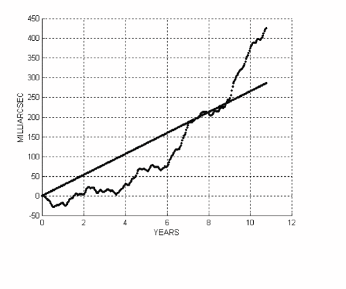
Figure 5: Simulation of our combined residuals of the nodes of LAGEOS and LAGEOS II using our combination. The residuals have been obtained using a highly unrealistic value of $\dot{J}_{4}$ equal to 611 $\%$ of the $\dot{J}_{4}$ value given in the EIGEN-GRACE02S model with x-intercept in 2000. The Lense-Thirring slope, fitting only for a secular trend, is $\mu\simeq 0.55$, i.e., it has a change of about 45 $\%$ with respect to the fit of Figure 2. The quadratic effect in the combined residuals due to $\dot{J}_{4}$ can be clearly identified even by visual inspection. This plot should be compared with Fig. 1 (the result of (Ciufolini and Pavlis 2004)) and with Fig. 4 where these simulated combined residuals have been fitted by including a quadratic term in order to fit for the $\dot{J}_{4}^{Effective}$ effect.

Indeed, in Fig. 5 we have shown the result of a simulation using, as an example, a value of $\dot{J}_{4}=-8.61\cdot 10^{-11}$, corresponding to the value given in the EIGEN-GRACE02S model $plus$ 12 times the error of $\dot{J}_{4}$ given in (?) (see below), for example with x-intercept in the year 2000. Not only, in this case, to get a 45 $\%$ error we would need an error in $\dot{J}_{4}$ that is 1200 $\%$ of what estimated in ref. (?), but any such error would produce a huge deformation of the final residuals that can be easily identified even by visual inspection of the combined residuals and, however, completely fitted for using a quadratic as shown in Fig. 4 and as previously explained. A 45 $\%$ error in the measured value of $\mu$ due to a superimposed quadratic effect looks as a clear nonsense! In other words, by comparing Fig. (5) with Fig. (1) (corresponding to our measurement (?)), it is clear that what is missing and misunderstood in (?) is that the only relevant secular effect that can mimic the Lense-Thirring effect is due to the errors in the values of the static $J_{2n}$ coefficients used in our analysis, whereas the $\dot{J}_{2n}$ will show up as quadratic effects and therefore large values of $\dot{J}_{2n}$ can be clearly identified over our long period of 11 years and can be fitted for, using a quadratic curve. For example, in the single, i.e., $\it not$ combined, residuals of the node of LAGEOS and of the node of LAGEOS 2 of Fig. 6 and 7 is clearly observed a long term variation in the trend that, since it disappears in the nodes combination of Fig. 1, can be identified as an anomalous increase in the Earth quadrupole moment, corresponding to the effect observed by Cox and Chao (?).

Finally, since the measurements of $\dot{J}_{2n}$ and $J_{2n}$ are completely independent (as previously explained), the corresponding errors are independent and this allowed us to take the RSS of these errors. Nevertheless, even by just adding up these errors we would get an error budget of 6.6 $\%$, well within our quoted range of 5 $\%$ to 10 $\%$.

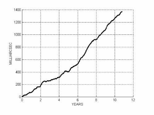
Figure 6: Residuals of the nodal longitude of LAGEOS using EIGEN-GRACE02S.

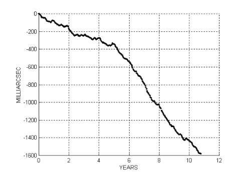
Figure 7: Residuals of the nodal longitude of LAGEOS 2 using EIGEN-GRACE02S.

Another way to look at the interconnection between the Lense-Thirring effect and the value of $\dot{J}_{4}$ is through a $\chi^{2}$ plot, as shown in Fig. 8. The origin of this graph corresponds to the best fit of our combined residuals by including a parabola in the fit (i.e., it corresponds to $\dot{J}_{4}^{Effective}\cong-1.41\cdot 10^{-11}-0.1\cdot 10^{-11}=-1.51\cdot 10^{-11}$ and Lense-Thirring effect $=98\%$ of the general relativity prediction) and the ellipse represents the confidence level (?) for a 99 $\%$ probability. It has to be stressed that this ellipse of confidence is tentative in the sense that we have assumed an average tentative standard deviation for each combined residual; the full analysis using the covariance matrix obtained by the GEODYN data reduction is presented in (?) . In this figure we have also included the value of $\dot{J}_{4}$ adopted in the EIGEN-GRACE02S model (?). The two parameters are indeed correlated, but this figure shows that the maximum uncertainty in the Lense-Thirring parameter arising from the possible variation of $\dot{J}_{4}$ is just $\sim\pm 0.75\%$ of its value. The complete error analysis published in (?) and (?) quotes a larger total uncertainty between 5 $\%$ and 10 $\%$ since it also takes into account all the other error sources.

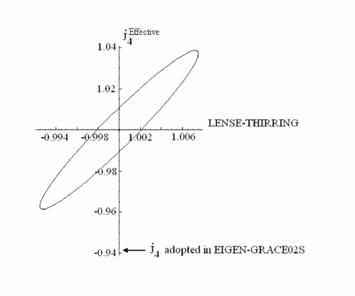
Figure 8: Confidence Ellipse. On the $x$ axis is the Lense-Thirring effect; the origin, at $x=1$, corresponds to the fitted value of frame-dragging. On the $y$ axis is $\dot{J}_{4}^{Effective}$; the origin, at $y=1$, corresponds to the fitted value $\dot{J}_{4}^{Effective}\simeq-1.51\cdot 10^{-11}$. This confidence ellipse is tentative since we have assumed an average tentative standard deviation for each combined residual. This figure shows that the maximum uncertainty in the measured Lense-Thirring parameter arising from the possible variation of $\dot{J}_{4}$ is just $\sim 0.75\%$

Let us estimate with a different method the maximum conceivable error due to the the $\dot{J}_{2n}$ in our measurement of the Lense-Thirring effect. First we stress that our error budget relies on the validity of the EIGEN-GRACE02S model and of the GRACE mission. Questioning our error budget is basically equivalent to question the validity of the GRACE mission itself.

As already pointed out, the Earth model EIGEN-GRACE02S was produced by GRACE measurements only, during the period 2002-2003, whereas the independent evaluation of $\dot{J}_{4}$ was produced on the basis of completely independent 30-year observations before 2002. The only constraint (based on the validity of the GRACE measurements) is that the $\dot{J}_{4}$ correction applied to $J_{4}$, must of course produce in 2002-2003 the same value of $J_{4}$ that was measured by GRACE in 2002-2003, at least within the EIGEN-GRACE02S uncertainties in $J_{4}$. Running then the orbital estimator GEODYN with or without a contribution corresponding to the estimated error in $\dot{J}_{4}$ of $\pm 0.6\cdot 10^{-11}$ (?) and by fitting the residuals without a parabola resulted in a change of the corresponding measured value of frame-dragging of $\pm$ 7.29 $\%$. This was verified in two ways: using GEODYN and an independent program written specifically to evaluate the $\dot{J}_{4}$ effect. By changing the observational period the measured value of frame-dragging would only slightly change (see the slope of Fig.1 over subsets of the total observational period of 11 years) and the corresponding error would consistently change too, increasing over periods farther away from 2002-2003. Nevertheless, over our observational period, the maximum $\dot{J}_{4}$ error was 7.29 $\%$. Similarly, by fitting the residuals without a parabola, an error of $0.5\cdot 10^{-11}$ in $\dot{J}_{6}$ would produce a 2.98 $\%$ error over our observational period. Then, by adding these errors to the error due to tides we get a maximum error of 11 $\%$ and finally considering all the other independent error sources (see the Supplementary Discussion of ref. (?)) we get a total uncertainty of 12 $\%$ in our measurement of the Lense-Thirring effect, in substantial agreement with the maximum error of about 10 $\%$ reported in (?). Nevertheless, it is critical to perform this worst case error analysis (without fitting our residuals with a quadratic) by using the most recent 2004 measurements of $\dot{J}_{4}$ and $\dot{J}_{6}$ (?), see also section 2. Recently, a solution for the time variation of the even zonal harmonics up to degree 6 was determined using Satellite Laser Ranging data from 8 geodetic satellites over a time period of 28 years from 1976 to 2003. The secular zonal variations for the degree up to 6 have been determined using the existing long term Satellite Laser Ranging data from multiple satellites, including Starlette, Ajisai, Stella, Lageos I and II, Etalon I and II, and BEC using both long and short arc orbital analysis technique. The results of (?) are $\dot{J}_{4}=-1.99\cdot 10^{-11}$ and $\dot{J}_{6}=0.02\cdot 10^{-11}$. Then, we have used these values of $\dot{J}_{4}$ and $\dot{J}_{6}$ and the orbital estimator GEODYN, according to the worst case analysis just described (without any fit for a quadratic term), to evaluate the impact of these different values of $\dot{J}_{4}$ and $\dot{J}_{6}$ in our measurement of the Lense-Thirring effect. We have then found a total difference of about 6.9 $\%$ in our measurement of the Lense-Thirring effect due to these new values of $\dot{J}_{4}$ and $\dot{J}_{6}$ (a precise statistical analysis based on the scatter of the various determinations of the $\dot{J}_{2n}$ is presented in a detailed paper in preparation (?)). Then, by adding this error to the error due to tides we get a maximum error of less than 7.9 $\%$ from time variations of the Earth gravity field and finally considering all the other independent error sources we get a total uncertainty of 9.3 $\%$ in our measurement of the Lense-Thirring effect, in full agreement with the maximum error of about 10 $\%$ reported in (?).

However, as explained above, we stress that the effect of such an error in $\dot{J}_{4}^{Effective}$ is not observed in our combined residuals, nor is of course observed a larger error of this type (?) that would in fact produce in our combined residuals a huge parabola superimposed to the frame-dragging trend (see, for example, Fig. 5). Indeed, as previously explained, by fitting our raw residuals including a quadratic curve we have that the total effect of the $\dot{J}_{2n}$, with ${2n}\geq 4$, on the combined node residuals corresponds to a total error in our determination of frame-dragging of about 1 $\%$ only.

It is finally worth to stress once again that the measured value of the Lense-Thirring effect, $\mu\cong 0.98$, obtained by fitting with a straight line and six periodic terms plus a parabola the raw combined residuals of (?), fit shown in Fig. 2, fully agrees with the measured value of the Lense-Thirring effect, $\mu\cong 0.98$, obtained by fitting with a straight line and six periodic terms plus a parabola the raw combined residuals simulated over our observational period of 11 years using GEODYN without inclusion of any $\dot{J}_{4}$, i.e. with $\dot{J}_{4}=0$ (Fig. 3), and with a highly unrealistic value of $\dot{J}_{4}=611\,\%\,{\dot{J}_{4}}^{EIGEN-GRACE02S}$ (Fig. 4).

In conclusion, the 5 $\%$ uncertainty in our measurement of the Lense-Thirring effect is fully confirmed in spite of the serious misunderstandings of our analysis in (?). Indeed, a number of further critical remarks are reported in (?) that show that his author did not carefully and seriously read our papers but only superficially read them and deeply misunderstood them.

In (?) is written “The value $\dot{J}_{4}^{eff}\cong-1.5\cdot 10^{-11}$ year^-1 measured with the combination of Eq. (5) is affected not only by $\dot{J}_{6}$ and the other higher degree even zonal harmonics but, more importantly, by the Lense Thirring signature itself. Indeed, the combination of Eq. (5) is designed in order to only disentangle $\dot{J}_{6}$ and the Lense Thirring effect. So, it is not admissible to use the so obtained $\dot{J}_{4}^{eff}$, which is coupled by construction to the Lense Thirring effect, in order to reliably and correctly measure the Lense Thirring effect itself” This statement is completely false because the Lense-Thirring effect was measured in (?), as very clearly written in (?), by only fitting with a straight line (plus the main periodical terms) the residuals produced with the standard value of $\dot{J}_{4}$ adopted in the EIGEN-GRACE02S model: no effective $\dot{J}_{4}$ and no quadratic fit were used in order to obtain our result in (?). The quadratic fit, together with a straight line and harmonics terms, was only used as a ”tool”, to evaluate the strength of any unmodelled $\dot{J}_{4}$ effect (as above explained in details). Furthermore, as clearly explained above, the statement “the so obtained $\dot{J}_{4}^{eff}$, which is coupled by construction to the Lense Thirring effect” is completely void of any possible meaning.

Furthermore, this paper (?) is not $properly$ referring to all the fundamental papers published since 1984 on the use of the nodes of the LAGEOS satellites in order to measure the Lense-Thirring effect (see section 4).

In the conclusion of (?) is written: “For a given observational time span and a given background reference Earth gravity model, two time series of the combined residuals, built up with and without the aforementioned $\dot{J}_{l}$ GTR-free values in the background reference models, it should be analyzed. The difference between the so obtained $\mu$ parameters can, then, be evaluated.” Again, in an official rebuttal letter of Ciufolini and Pavlis, dated November 2004 (?), to answer one of the papers of criticism sent by Iorio for publication (rejected by the referees), the method to evaluate the impact of the $\dot{J}_{2n}$ uncertainties was clearly written and explained: “ … Running then the orbital estimator GEODYN with or without a contribution corresponding to the estimated error in $\dot{J}_{4}$ of $0.6\cdot 10^{-11}$ (?) resulted in a change of the corresponding measured value of frame-dragging by 7.29 $\%$. …”. This is exactly one of the methods of error analysis reported here.

However, the most profound misunderstanding in (?) is the following “… If one is interested in extracting from such a signal a linear trend, it is not possible also to fit a parabolic noise signal without corrupting or distorting in some way the genuine linear trend of interest. Exactly in the same way, it is not possible to fit and remove the noise linear signal induced by $J_{4}$, $J_{6}$, . . . It is only possible to evaluate, as more accurately and realistically as possible, their impact on the measurement of the linear trend.”. In a previous similar paper of the same author (?) is written: “The time series of the combined residuals of the nodes of LAGEOS and LAGEOS II consists of the Lense-Thirring linear trend as predicted by GTR, which has, in fact, to be measured, the linear trend induced by the static part of the uncancelled even zonal harmonics of the geopotential $J_{4}$, $J_{6}$ …, the parabolic signal induced by $\dot{J}_{4}$, $\dot{J}_{6}$ and the time-varying harmonic perturbations of gravitational and non gravitational origin. If one is interested in extracting from such a signal a linear trend, modelled as $a_{0}+a_{1}t$, it is not possible also to fit a parabolic noise signal, modelled as $b_{0}+b_{1}t+b_{2}t^{2}$, without corrupting or distorting in some way the genuine linear trend of interest. …”.

However, in the above mentioned official letter of Ciufolini and Pavlis to Iorio, dated November 2004 (?), it was clearly written: “First, our error budget relies on the validity of the EIGEN-GRACE02S model and of the GRACE mission. Questioning our error budget is equivalent to questioning the validity of the GRACE mission itself. We stress that the Earth model EIGEN-GRACE02S was produced by GRACE measurements ONLY, during the period 2002-2003, whereas the INDEPENDENT evaluation of $J_{4}$-dot was produced on the basis of completely independent 30-year observations BEFORE 2002. The only constraint (based on the validity of the GRACE measurements) is that the $J_{4}$-dot correction applied to $J_{4}$, MUST of course produce in 2002-2003 the same value of $J_{4}$ as that was measured by GRACE in 2002-2003.”

This means that one is not free to fit for a trend $b_{1}t$ due to $\dot{J}_{4}$ in addition to the trend $a_{1}t$ but, on the basis of the 2002-2003 GRACE measurement of $J_{4}$, any change $\dot{J}_{4}$, when applied to the EIGEN-GRACE02S static model, must of course be such to agree in 2002-2003 with the value of $J_{4}$ measured by GRACE in 2002-2003 (at least within the small measurement uncertainty given in the EIGEN-GRACE02S model; this small uncertainty has however a negligible influence on our final result). This means that, since we have to be consistent with the GRACE observation of $J_{4}$ in 2002-2003, the term $b_{1}$ must be: $b_{1}\equiv-2b_{2}N$, where N is the number of years between the first year of application of the $\dot{J}_{4}$ correction and the GRACE observations in 2002-2003. Therefore, as we did, one only needs to fit for $b_{2}$ and get $b_{1}$ from it, or alternatively (as we also did) fit for $b_{2}(t^{2}-2Nt)$ in addition to the $a_{1}t$ trend. So our test fit is just a polynomial fit (with or without the periodic terms). In conclusion, in the two sections reported above, the author of (?) is explicitly stating that one cannot fit some observational data with a polynomial of degree three!!

2 On the value of $\dot{J_{4}}$

Long period and secular variations in the zonal harmonics of the spherical harmonic expansion describing Earth’s gravitational field are generally attributed to “post-glacial rebound” and ice-sheet mass changes (?, ?, ?), and reflect changes in Earth’s viscous lower mantle (?). These changes hold information about the dynamics of Earth and its anelastic response to tidal forcing. Estimation of the secular rates for the zonal harmonics therefore has been a high priority research topic of space geodesy for many years now, with a considerable number of independent results in the literature (?, ?, ?, ?, ?, ?, ?, ?, ?, ?, ?, ?, ?, ?, ?). The majority of these results were obtained from the analysis of long time intervals spanning several decades of data obtained from several satellites including the two LAGEOS, Starlette, Ajisai, Stella, BE-C and the two ETALONs. Due to the limited number of satellite orbit configurations, only a handful of the very lowest degree zonal terms’ rates can be “observed” (?), reaching at best, up to degree six. The estimation of the zonal rates is in most cases based on perturbation analysis of very long arcs (several years), but not always necessarily so. In particular, the last four studies cited above involve short-arc techniques, estimating the average “static” value of the zonal harmonics, and deriving the rate from a subsequent analysis of the resulting time series. Furthermore, in most cases, the investigators used their static gravitational model of preference, implying that the adopted epoch values for $J_{4}$ were different amongst studies. These differences are well documented in the literature dealing with the static models JGM-3, EGM96, GRIM5-S1, TEG-4, EIGEN-GRACE02S, and GGM01S. It is then remarkable that from a plethora of approaches, analyzed data sets, and diverse analysis s/w packages used, the resulting estimate for the secular rate of these harmonics, e.g. $\dot{J}_{4}$, which is of interest here, differs by no more than 100% from the commonly accepted value (?), the one that was also used in the development of EIGEN-GRACE02S.

As it is discussed in (?), there is considerable correlation between the zonal rate estimates ($\rho_{\dot{J_{2}},\dot{J_{4}}}=-0.75,\rho_{\dot{J_{2}},\dot{J_{6}}}=+0.76,\rho_{\dot{J_{4}},\dot{J_{6}}}=-0.86$), but there is no significant correlation between the static values of the harmonics and their rates. This independence of errors between the static values’ estimates and the associated rates is further demonstrated in (?), where monthly estimates of the $J_{2}$ term obtained from GRACE data and those obtained entirely independently from SLR data analysis are compared. The agreement is remarkable, even though the GRACE data analysis has not reached yet its definitive level. The results from (?) suggest that the current best estimate for $\dot{J_{4}}$, with all other zonal rates up to $\dot{J_{6}}$ simultaneously estimated, is $-1.99\times 10^{-11}$/y. This value is only $0.58\times 10^{-11}$/y off the currently accepted value, adopted in developing EIGEN-GRACE02S, or in terms of a percentage, it is off by only -41%. This possible range of error is well within our $\mu$ error margin (5-10%), since our simulation of a 611% error in $\dot{J_{4}}$ resulted only in a corresponding 1% error in the fitted value of $\mu$.

A careful collection of all the published values of $\dot{J_{4}}$ in the literature and subsequent statistical analysis, points to the same conclusion. Since the published estimates can be in most cases considered independent as we explained above, we can perform a simple statistical analysis of these values and their variance in comparison to the quoted error estimates of these values. The population is not large by any statistical standards, but that is what is available. There are two estimates, $+0.2\times 10^{-11}$ (?) and $+0.3\times 10^{-11}$ (?), which are clearly outliers and the reasons are explained in (?), so our statistical tests include cases where both of these or either one separately are eliminated from the population of estimates. The results in terms of a mean $\dot{J_{4}}$ and its associated scatter are shown in Table 1.

Table 1: Statistical significance of the variations between individual $\dot{J_{4}}$ estimates.

Case Description	Mean value of $\dot{J_{4}}$	Scatter of $\dot{J_{4}}$	References
	($\times 10^{-11}$/y)	($\times 10^{-11}$/y)
A. Six estimates
from Table 5
(ref. 1) and
the new estimate
from (ref. 2)	-0.70	$\pm$0.8	(1): (?)
			(2): (?)
B. As in A,
but without
the two outliers
of +0.2 and
$+0.3\times 10^{-11}$/y	-1.02	$\pm$0.6	As in (A).
C. As in A,
removing only
the estimate of
$+0.3\times 10^{-11}$/y	-0.84	$\pm$0.74	As in (A).
D. As in A,
removing only
the estimate of
$+0.2\times 10^{-11}$/y	-0.83	$\pm$ 0.76	As in (A).
E. Nine estimates
from Table 7
of Ref. 1.	-1.697	$\pm$0.69	(1): (?)

These tests point to one conclusion very clearly: the uncertainty in our present knowledge of $\dot{J_{4}}$ is in the neighborhood of $\pm 0.7\times 10^{-11}$/y and this quantity is only 50% of the $\dot{J_{4}}$ value that we used in our Lense–Thirring measurement. It implies that with a 67% probability, the true value of $\dot{J_{4}}$ could be in the interval [-1.697 - 0.7 to -1.697 + 0.7] , that is [-2.4, -1.0], or if we increase the probability to 95% confidence level, we then have the corresponding interval of [-3.1, -0.3], or even at the 99% level, $\dot{J_{4}}$ will then lie in the interval [-3.8, +0.4], all values in $10^{-11}$/y.

From all these cases, we see that we never reach the extreme valueon: $-8.61\times 10^{-11}$/y, although, even in that case, the final effect on the fitted value of $\mu$ was only 1%!

In conclusion, from all the cases studied, there is no reason to expect an error in $\dot{J_{4}}$ of more than $0.7\times 10^{-11}$/y (at 1-$\sigma$ level of significance, i.e. 67% probability), and all statistically acceptable variations in the estimate of $\dot{J_{4}}$ indicate that there can be no more than 1% error in the fitted value of $\mu$, caused by this error in $\dot{J_{4}}$, as shown in section 1. The evaluation of the $\dot{J_{4}}$ error estimate on the basis of the various results indicates also a perfect agreement with the quoted $1\times 10^{-11}$/y error for the $-1.41\times 10^{-11}$/y rate for $J_{4}$, which was adopted in developing EIGEN-GRACE02S.

3 “Imprint” or “Memory” of the Lense-Thirring Effect

In regard to other conceivable error sources, a possible bias in our measurement of $\mu$ might be due to some “imprint” or “memory” of the a priori value of the Lense–Thirring effect used in the determination of the gravity model [see: (?)]. The author of (?) is mentioning this potential source of error in section 3.2.6 “The a priori “memory” effect of the Lense Thirring signature on the adopted Earth gravity model on the Earth gravity model used”. The Earth gravity field model EIGEN-GRACE02S has been obtained using the observations of the GRACE satellites only and by using a set of models and parameters to describe the orbital perturbations, including some a priori, theoretical, value of the Lense–Thirring effect, indeed EIGEN-GRACE02S has been obtained without the Lense-Thirring effect in the data analysis. The previous models EIGEN-2S and GGM01S have been derived using the observations of the CHAMP and GRACE satellites. Thus, the gravitational field model EIGEN-GRACE02S that we used to measure $\mu$ may contain some kind of “imprint” of the a priori, theoretical, value of the Lense–Thirring effect (i.e., zero in the EIGEN-GRACE02S case).

Nevertheless, in the present analysis we are only concerned about a conceivable imprint on the Earth’s even zonal harmonics $J_{2n}$. The Earth gravitational potential is measured by observation of the rate of change of the GRACE inter-satellite distance (?), i.e., the gravitational field is measured by observation of the relative acceleration of two test particles (the equation linking relative acceleration and gravitational field is, in general relativity, the geodesic deviation equation (?)). However, the effect of the gravitomagnetic field on the acceleration vector of a satellite (?), decomposed in out–of–plane direction, $\bot$ (orthogonal to the satellite orbital plane); along track, $\hat{\bf{v}}$ (along the satellite velocity vector); and radial direction, $\hat{\bf{r}}$ (along $\bf{r}$), is given by $\bf{a}=\bf{v}\times\bf{H}$, where ${\bf H}\,=\,{{{2\,[{\bf J}\,-\,3\,({\bf J}\,\cdot\,\hat{\bf x}\,)\,\hat{\bf x}]}\over{|{\bf x}|^{3}}}}$ is the gravitomagnetic field and ${\bf{v}}=v\bf\hat{v}$. For a polar satellite with a circular orbit we then have $a^{L-T}_{\bot}\sim\sin\phi$, where $\phi$ is the latitude, $a^{L-T}_{\hat{\bf{r}}}=0$ and $a^{L-T}_{\hat{\bf{v}}}=0$. However, the effect of the even zonal harmonics on the acceleration vector of a satellite is given by $\bf{a}={\bf{\nabla}}U$ and the terms of the potential $U$ generated by the mass, $M$, of the central body and by the even zonal harmonics, $J_{2n}$, are (?): $U={M\over r}\,[1-J_{2}\,({R_{\oplus}\over r})^{2}P_{20}(\sin\phi)-J_{4}({R_{\oplus}\over r})^{4}P_{40}(\sin\phi)-...]$, where $J_{2}$ and $J_{4}$ are the non–normalized even zonal harmonic coefficients of degree 2 (quadrupole) and 4, $R_{\oplus}$ is the Earth’s equatorial radius and $P_{20}(\sin\phi)$ and $P_{40}(\sin\phi)$ are the Legendre associated functions. For a polar satellite with a circular orbit we then have $a^{J_{2n}}_{\bot}=0$, $a^{J_{2n}}_{\hat{\bf{r}}}\neq 0$ and $a^{J_{2n}}_{\hat{\bf{v}}}\neq 0$. Then, for a polar satellite with a circular orbit the satellite acceleration generated by the even zonal harmonics is just orthogonal to satellite acceleration generated by the gravitomagnetic field (i.e. the Lense–Thirring effect). In conclusion, the static even zonal harmonics determined by a polar satellite with a circular orbit are independent on the a priori value used for the Lense–Thirring effect.

Indeed, the orbit of the GRACE satellites is nearly circular with eccentricity $<0.005$ (the same is true for the CHAMP satellite with eccentricity = 0.004) and basically polar with inclination = 89^∘ (the same is true for the CHAMP satellite with inclination = 87.3^∘), thus the values of the even zonal harmonics determined by the GRACE orbital perturbations are substantially independent on the a priori value of the Lense–Thirring effect. This also applies to the CHAMP polar satellite and to the previous CHAMP and GRACE only models. The small deviation from a polar orbit of the GRACE satellite, that is $1.7\times 10^{-2}$ rad, gives only rise, at most, to a very small correlation with a factor $1.7\times 10^{-2}$. For CHAMP this correlation is, at most, $\sim$ $4.7\times 10^{-2}$. In addition, since our results are independent of the error in the quadrupole coefficient $J_{2}$, any bias in $J_{2}$ due to a Lense–Thirring “imprint” is canceled in our combination (4). However, the Lense–Thirring effect depends on the third power of the inverse of the distance from the central body, i.e., $(1/r)^{3}$, and the $J_{2}$, $J_{4}$, $J_{6}$ … effects depend on the powers $(1/r)^{3.5}$, $(1/r)^{5.5}$, $(1/r)^{7.5}$ … of the distance; then, since the ratio of the semimajor axes of the GRACE satellites to the LAGEOS’ satellites is $\sim\;{6780\over 12270}\cong{1\over 1.8}$, any conceivable “Lense–Thirring imprint” on the spherical harmonics at the GRACE altitude becomes quickly, with increasing distance, a negligible effect, especially for higher harmonics of degree $l\geq 4$. Therefore, any conceivable “Lense–Thirring imprint” is negligible at the LAGEOS’ satellites altitude. The same applies to the CHAMP polar satellite. In addition, in (?), it was proved with several simulations that by far the largest part of this “imprint” effect is absorbed in the by far largest coefficient $J_{2}$.

In conclusion, any error due to a conceivable “imprint” of the Lense–Thirring effect on the Earth’s even zonal harmonics of the EIGEN-GRACE02S model (and of the other CHAMP and GRACE only models) is negligible on the combination (4) of the nodes of LAGEOS and LAGEOS II and therefore in our measurement of the Lense-Thirring effect.

4 A brief history of proposed experiments and measurements of the Lense-Thirring effect using the nodes of the LAGEOS satellites

The measurement reported in Nature (?) uses the nodes of the two laser ranged satellites LAGEOS and LAGEOS 2 in order to cancel the effect of the first even zonal harmonic coefficient, $J_{2}$, of Earth and to measure the Lense-Thirring effect. Furthermore, it uses the accurate model EIGEN-GRACE02S of the Earth gravity field developed by GFZ of Potsdam with the data of the NASA GRACE satellites.

The key idea of using the nodes of two laser ranged satellites of LAGEOS type to measure the Lense-Thirring effect was published for the first time in 1984-86 (?, ?)).

The idea to use the nodes of N satellites of LAGEOS type to cancel the effect of the first N-1 Earth even zonal harmonics and to measure the Lense-Thirring effect was published for the first time in 1989 (?). The measurement of the Nature paper is simply the case of N=2. Indeed, in this 1989 paper on page 3102, fourth line, in order to measure the Lense-Thirring effect and to cancel the even zonal harmonics uncertainties, it is proposed (see also (?), on page 336): “For $J_{2}$, this corresponds from formula (3.2), to an uncertainty in the nodal precession of 450 milliarcsec/year, and similarly for higher $J_{2n}$ coefficients. Therefore the uncertainty in $\dot{\Omega}_{Class}^{Lageos}$ is more than ten times larger than the Lense-Thirring precession. A solution would be to orbit several high-altitude, laser-ranged satellites, similar to LAGEOS, to measure $J_{2},J_{4},J_{6}$ etc, and one satellite to measure $\dot{\Omega}_{Lense-Thirring}$ ”. Thus, the case of the Nature paper is just the one with two satellites. At that time the error due to the even zonal harmonics was quite larger due to the much less accurate Earth gravity models available at that time and the LAGEOS 2 satellite was not yet launched (it was launched in 1992).

In particular, the idea, to use the two nodes of the satellites LAGEOS and LAGEOS 2 to measure the Lense-Thirring effect, together with the corresponding formula also using the perigee of LAGEOS 2, was published for the first time in 1996 (?). See, e.g., the formula (15) on page 1717 of ref. (?): “$\delta\dot{\Omega}_{I}+k_{1}\delta\dot{\Omega}_{II}+k_{2}\delta\dot{\omega}_{II}=\mu(31+31.5k_{1}-57k_{2})\,milliarcsec/year\,+\,[other\,error\,sources\,(\delta C_{60},\delta C_{80},...,\delta I_{I},\delta I_{II})],$” in the slightly different notation of the Nature paper this is exactly eq. (1) of (?) where 31 and 31.5 are written in the Nature paper: $\dot{\Omega}_{I}^{Lense-Thirring}$ and $\dot{\Omega}_{II}^{Lense-Thirring}$ and $\delta C_{60},\delta C_{80}$, … are just written $\Sigma\delta J_{2n}$, and $k_{2}=0$, i.e. there is no use of the perigee, but just of the nodes, according to what we suggested in the above 1989 paper (?) and similar following papers. All the relevant LAGEOS and LAGEOS 2 nodal rate coefficients of the $J_{2n}$, up to $J_{4}$, were explicitly given in this 1996 paper.

In (?) various combinations of the orbital elements of the satellites LAGEOS, LAGEOS 2 and LAGEOS 3 were also studied.

Finally, the combination (1) of ref. (?), using the nodes only, with the explicit value of the $k_{1}$ coefficient (that is however an absolutely trivial step using the above formula and the coefficients given in (?), since it corresponds to set $k_{2}=0$, according to what explained in (?) and (?), and to carry out the following highly trivial arithmetics: $k_{1}\cong-(-9.3/17.2)\cong 0.54$, where the coefficients $K_{20}^{I}\cong-9.3\cdot 10^{11}$ milliarcsec/yr and $K_{20}^{II}\cong 17.2\cdot 10^{11}$ milliarcsec/yr were explicitly given in (?)) was presented and published in the SIGRAV 2002 Villa Mondragone (Rome) School proceedings (?), presented at a plenary talk at the Marcel Grossmann meeeting in Rio de Janeiro in July 2003 (to appear in the proceedings (?)) and at a number of other meetings since 2002. In almost every talk given by one of us from 1996 to 2004, it was discussed the possibility of using the nodes only of LAGEOS and LAGEOS 2 to just cancel the $J_{2}$ effect and measure the Lense-Thirring effect. Therefore, the author of (?) seems to have just rediscovered in 2003-2004 what already published by one of us many years ago.

The use of the GRACE-derived gravitational models, when available, to measure the Lense-Thirring effect with accuracy of a few percent was, since many years, a well known possibility to all the researchers in this field and was presented by one of us during the SIGRAV 2000 conference (?) and published in its proceedings, and was published by Ries et al. in the proceedings of the 1998 William Fairbank conference and of the 2003 13th Int. Laser Ranging Workshop (?, ?), as very clearly reported in the Supplementary Discussion of (?) where it is written: “… (see also ref. [10] by Ries et al.-2003 concluding that, in the measurement of the Lense-Thirring effect using the GRACE gravity models and the LAGEOS and LAGEOS 2 satellites: “a more current error assessment is probably at the few percent level”) …”.

In conclusion, all the claims of the author (?) are simply lacking of any rational basis: above is shown how much work was already published on this topic before the author of (?) even began to produce any of his paper on this topic and to rediscover some earlier results (the papers reported above are just a small subset of all the work published by us in the last 20 years). To avoid the misunderstandings of (?), it would have just been a matter of very carefully reading the previously existing literature on this subject!

Let us finally briefly comment on some historical milestones in regard to the error analysis of the Nature paper and to the uncertainties in the perturbations of the nodes of the LAGEOS satellites.

The error analysis of our 2004-measurement of the Lense-Thirring effect with the LAGEOS and LAGEOS 2 satellites is substantially the same as the error analysis of the LAGEOS III/LARES experiment that was carried out in a very large number of papers and studies of NASA, ASI and ESA (?). In particular, in 1989, this analysis was performed under the supervision of an official NASA committee chaired by Peter Bender, with members J. Anderson, J. Armstrong, J. Breakwell, D. Christodoulidis, F. Everitt, E. Guinan, R. Hellings, R. King, I. Shapiro, D. Smith and R. Weiss; then, in 1994, J. Ries et al., published a revised error budget of the LAGEOS III experiment, with a total error of 4 $\%$ [this 1994 error analysis of Ries et al. is reported with its reference in the Supplementary Discussion of (?)] and, in 1998, with a total error of 3$\%$-4$\%$ [see: (?) in (?)], as reported in the Supplementary Discussion of (?).

For differences and similarities between the error analysis of the proposed LAGEOS III/LARES experiment and the one of the recent measurement of the Lense-Thirring effect with LAGEOS and LAGEOS 2 (?), see the Supplementary Discussion of (?) and ref. (?). Here we just stress that the studies of the LAGEOS III/LARES experiment were fundamental milestones in this field, indeed they analyzed in details all the main modelling errors in the nodal rates of LAGEOS type satellites.

5 On the use of the mean anomaly and on the use of Jason to measure the Lense-Thirring effect proposed in (Iorio 2004)

Besides the deep misjudgements and miscalculations of the impact of $\dot{J}_{4}$ and of any “Lense-Thirring imprint” in the uncertainty of our measurement of frame-dragging, one of the most profound mistakes and misunderstandings of (?) is the proposed use of the mean anomaly of a satellite to measure the Lense-Thirring effect (in some previous paper by the same author the use of the mean anomaly was also explicitly proposed; see e.g. L. Iorio ”Some comments on the recent results about the measurement of the Lense-Thirring effect in the gravitational field of the Earth with the LAGEOS and LAGEOS II satellites” arXiv:gr-qc/0411084 $\bf{v5\;19\;Apr\;2005}$, however its latest versions, after the online publishing of our present paper in New Astronomy on the 2nd of May 2005, have been amended of this mistake). In (?) (arXiv:gr-qc/0411024 $\bf{v9\;19\;Apr\;2005}$, however its latest versions, after the online publishing of our present paper in New Astronomy on the 2nd of May 2005, have been amended of this mistake) is written:

“The problem of reducing the impact of the mismodelling in the even zonal harmonics of the geopotential with the currently existing satellites can be coped in the following way. Let us suppose we have at our disposal N $(N>1)$ time series of the residuals of those Keplerian orbital elements which are affected by the geopotential with secular precessions, i.e. the node, the perigee and the mean anomaly: let them be $\Psi^{A}$, A = LAGEOS, LAGEOS II, etc. Let us write explicitly down the expressions of the observed residuals of the rates of those elements $\delta\dot{\Psi}^{A}_{obs}$ in terms of the Lense Thirring effect $\dot{\Psi}^{A}_{LT}$, of N - 1 mismodelled classical secular precessions $\dot{\Psi}^{A}_{l}\delta J_{l}$ induced by those even zonal harmonics whose impact on the measurement of the gravitomagnetic effect is to be reduced and of the remaining mismodelled phenomena $\Delta$ which affect the chosen orbital element:

$$\delta\dot{\Psi}^{A}_{obs}=\delta\dot{\Psi}^{A}_{LT}+\Sigma\dot{\Psi}^{A}_{l}\delta J_{l}+\Delta^{A},$$

$$A=LAGEOS,LAGEOSII,...\;\;\;\;\;(2)$$

The parameter${}^{7}\;\mu$ is equal to 1 in the General Theory of Relativity and 0 in Newtonian mechanics. The coefficients $\dot{\Psi^{A}_{l}}$ are defined as

$$\dot{\Psi}_{l}={{\partial\dot{\Psi}_{class}}\over{\partial J_{l}}}\;\;\;\;\;(3)$$

and have been explicitly worked out for the node and the perigee up to degree $l=20$ in Iorio (2002b, 2003a); they depend on some physical parameters of the central mass (GM and the mean equatorial radius $R$) and on the satellite’s semimajor axis $a$, the eccentricity $e$ and the inclination $i$. We can think about Eq. (2) as an algebraic non-homogeneuous linear system of N equations in N unknowns which are $\mu$ and the N - 1 $\delta J_{l}$: solving it with respect to $\mu$ allows to obtain a linear combination of orbital residuals which is independent of the chosen N - 1 even zonal harmonics.”

This is simply a nonsense paragraph: let us, for example, consider a satellite at the LAGEOS altitude, the Lense-Thirring effect on its mean longitude is of the order of 2 meters/yr, however the mean longitude change is about $1.8\cdot 10^{11}$ meters/yr. Thus, from Kepler’s law, the Lense-Thirring effect corresponds to a change of the LAGEOS semi-major axis of about 0.09 millimeters. Since, even a high altitude satellite such as LAGEOS showed a semimajor axis change of the order of 1 millimeter/day, due to atmospheric drag and to the Yarkoski-Rubincam effect (because of atmospheric drag, the change of semimajor axis and mean motion is obviously much larger for lower altitude satellites), and since the present day $precision$ of satellite laser ranging is, even in the case of the best SLR stations, of several millimeters, it is a clear nonsense to propose a test of the Lense-Thirring effect based on using the mean anomaly of ANY satellite, mean anomaly largely affected by non-conservative forces.

In (?) and in one of Iorio’s recent papers, it is proposed to use the data collected from the satellite mission JASON, to accurately measure the Lense-Thirring effect. Let us highlight some of the major obstacles that one would face in trying to implement such a proposal. A more detailed work discussing this proposal, the use of the mean anomaly and other highly unfeasible proposals of the author of (?) will be the subjects of a following paper.

First of all, Jason is a “low Earth orbit” satellite, at a 1330 km altitude, and experiences by far larger perturbations than the LAGEOS satellites from atmospheric drag, albedo and solar radiation pressure and from all gravitational wavelengths. The complicated shape of the satellite makes impossible to precisely “forward-model” all the non-conservative forces acting on the satellite which generate perturbations that are making JASON a totally unsuitable target for making a measurement of such a tiny effect as the Lense-Thirring drag.

JASON is an oceanographic mission which measures radar ranges from the satellite to the surface of the ocean with a precision of about 4 cm. To make use of these observations for oceanographic research, the requirement on the orbital accuracy is stringent but certainly not extraordinary. A couple of centimeters of radial error are adequate, although recent results indicate that we may be closer to 1 cm (?). The JASON bus is a very large, asymmetrical one and it was not designed to support millimeter ranging work, since oceanography is still trying to rationalize much larger signals. In addition to the large size and poorly defined shape in terms of properties, etc., the satellite undergoes nearly continuous orbital adjustments to maintain its ground-track within $\pm$ 1 km off the accepted mean ground-track of the Topex/Poseidon mission and in this process its ideal orbit as a test particle in the Earth gravitational field changes by thrusting and maneuvering; this is never easily controlled and it cannot be taken into account in computing a perfectly reconstituted orbit. The shape of the satellite bus and the continuous motion of parts on the bus (e.g., solar panels) as well as the satellite itself (yawing or not, to maintain orientation with respect to the Sun) generate further accelerations that are unknown and extremely difficult to account for, except by solving for what we call “ad hoc”, non-physically meaningful, accelerations at certain intervals and that, however, will absorb signals such as the L-T effect. To avoid these problems a large international group of researchers proposed the LARES/WEBERSAT mission (?) and, in doing so, designed a new structure for the LARES satellite, a very clean cannonball satellite, similar to LAGEOS but improved for what regards the effect of the non-gravitational perturbations. In any case, one wonders why the author of (?) has not proposed the use of which not only have by far better shape and orbital stability compared to JASON but they also carry ultra precise accelerometers that measure all non-conservative accelerations, so that they are in practice “free-falling” particles in vacuum, at least to the extent that is covered by the accuracy of these instruments.

In conclusion, not only all the criticisms in Iorio’s paper are completely unfounded and misdirected and our total error bubget is fully confirmed to be between 5 $\%$ and 10 $\%$ of the Lense-Thirring effect, but Iorio’s paper shows a profound lack of understanding and knowledge of the real, practical, data analysis of laser ranging observations and of the actual modeling of the Earth gravity field.

Acknowledgements

One of us (I.C.) is very grateful to Richard Matzner for reading the manuscript and for helpful suggestions.

References

- [1]
- [2] [] Ciufolini, I., and Pavlis, E., Letters to Nature, 431, 958 (2004).
- [3]
- [4] [] Reigber, C., Schmidt, R., Flechtner, F., Konig, R., Meyer, U., Neumayer, K. H., Schwintzer, P., and Zhu, S. Y., J. Geodyn. 39, 1 (2005). The EIGEN-GRACE02S gravity field coefficients and their calibrated errors are available at: http://op.gfz-potsdam.de/grace/index_GRACE.html 18.
- [5]
- [6] [] Eanes, R. J., A study of temporal variations in Earth’s gravitational field using Lageos-1 laser ranging observations. Ph.D. Dissertation. The University of Texas at Austin, 1995.
- [7]
- [8] [] Iorio, L., New Astronomy, in the press, 2005, doi: 10.1016/j.newast.2005.01.001.
- [9]
- [10] [] Ciufolini, I., Pavlis, E., and Peron, R., to be published (2005)
- [11]
- [12] [] Cox, C. M., and Chao, B., Science, 297, 831 (2002).
- [13]
- [14] [] Press, W. H., Flannery, B. P., Teukolsky, S. A., and Vetterling, W.T., Numerical Recipes (Cambridge University Press, Cambridge, New Jersey, 1986).
- [15]
- [16] [] Ciufolini, I., Pavlis, E., et al., in preparation (2005)
- [17]
- [18] [] Cheng, M. K. and Tapley, B. D., Secular variations in the low degree zonal harmonics from 28 years of SLR data, AGU Fall Meeting Abstracts, C801 (2004).
- [19]
- [20] [] Iorio, L., arXiv:gr-qc/0412057 v1, 12 Dec 2004.
- [21]
- [22] [] Ciufolini, I., and Pavlis, E., official letter of answer to the unpublished comments of Iorio on (?) submitted for publication.
- [23]
- [24] [] Trupin, A. S., Meier, M. F., and Wahr, J. M., Geophysical Journal International 108, 1 (1992).
- [25]
- [26] [] Ivins, E. R., Sammis, C. G., and Yoder, C. F., J. Geophys. Res. 98, 4579 (1993).
- [27]
- [28] [] Mitrovica, J. X. and Peltier, W. R., J. Geophys. Res. 98, 4509 (1993).
- [29]
- [30] [] Yoder, C. F., Williams, J. G., Dickey, J. O., Schutz, B. E., Eanes, R. J., and Tapley, B. D., Nature 303, 757 (1983).
- [31]
- [32] [] Rubincam, D. P., J. Geophys. Res. 89, 1077 (1984).
- [33]
- [34] [] Cheng, M. K., Eanes, R. J., Shum, C. K., Schutz, B. E., and Tapley, B. D., Geophys. Res. Lett. 16, 393 (1989).
- [35]
- [36] [] Gegout, P. and Cazenave, A., Geophys. Res. Lett. 18, 1739 (1991).
- [37]
- [38] [] Nerem, R. S., Chao, B. F., Au, A. Y., Chan, J. C., Klosko, S. M., Pavlis, N. K., and Williamson, R. G., Geophys. Res. Lett. 20, 595 (1993).
- [39]
- [40] [] Cheng, M. K., Tapley, B. D., Eanes, R. J., and Shum, C. K., Time-varying gravitational effects from analysis of measurements from geodetic satellite (abstract), EoS Trans. AGU, 74(43), Fall Meet., Suppl., p. 196 (1993).
- [41]
- [42] [] Cazenave, A., Gegout, P., and Ferbat, G., Secular variations of the gravity field from LAGEOS 1, LAGEOS 2 and AJISAI, Global Gravity Field and its Temporal Variations, Int. Assoc. of Geod. Symp. Vol. 116 (New York), Springer-Verlag, pp. 141–151 (1996).
- [43]
- [44] [] Nerem, R. S. and Klosko, S. M., Secular variations of the zonal harmonics and polar motion as geophysical constraints, Global Gravity Field and its Temporal Variations, Int. Assoc. of Geod. Symp. Vol. 116 (New York), Springer-Verlag, pp. 152–163 (1996).
- [45]
- [46] [] Eanes, R. J. and Bettadpur, S. V., Temporal variability of earth’s gravitational field from satellite laser ranging observations, Global Gravity Field and its Temporal Variations, Int. Assoc. of Geod. Symp. Vol. 116 (New York), Springer-Verlag, pp. 30–41 (1996).
- [47]
- [48] [] Cheng, M. K., Shum, C. K., and Tapley, B. D., J. Geophys. Res. 102, 22377 (1997).
- [49]
- [50] [] Devoti, R., Luceri, V., Rutigliano, P., Sciarretta, C., and Bianco, G., Bollettino DI Geofisica Teorica ED Applicata 40, 353 (1999).
- [51]
- [52] [] Cox, C. M., Klosko, S. M., and Chao, B. F., Changes in ice-mass balance inferred from time variation of the geopotential observed through slr and doris tracking, Gravity, Geoid and Geodynamics 2000, International Association of Geodesy (IAG) Symposia Volume 123 (M. G. Sideris, ed.), Springer (2000).
- [53]
- [54] [] Pavlis, E. C., Dynamical determination of origin and scale in the earth system from satellite laser ranging, Vistas for Geodesy in the New Millennium, Proc. 2001 International Association of Geodesy Scientific Assembly, Budapest, Hungary, September 2-7, 2001 (New York) (J. Adam and K.-P. Schwarz, eds.), Springer-Verlag, pp. 36–41 (2002).
- [55]
- [56] [] Cheng, M. K. and Tapley, B. D., J. Geophys. Res. 109, 9402 (2004).
- [57]
- [58] [] McCarthy, D. D. and Petit, G. (eds.), 2004. Iers conventions (2003), IERS Technical Note 32, Observatoire de Paris, Paris (2004).
- [59]
- [60] [] Ciufolini, I., et al., Class. and Quantum Grav. 14, 2701 (1997).
- [61]
- [62] [] Kaula, W. M., Theory of Satellite Geodesy, (Blaisdell, Waltham, 1966).
- [63]
- [64] [] Ciufolini, I., “Theory and Experiments in General Relativity and other Metric Theories” Ph. Dissertation, Univ. of Texas, Austin, Ann Arbor, Michigan, 1984.
- [65]
- [66] [] Ciufolini, I., Phys. Rev. Lett. 56, 278 (1986).
- [67]
- [68] [] Ciufolini, I., Int. J. Mod. Phys. A 4, 3083 (1989).
- [69]
- [70] [] Ciufolini, I., and Wheeler, J.A., Gravitation and Inertia (Princeton University Press, Princeton, New Jersey, 1995).
- [71]
- [72] [] Ciufolini, I.,, Nuovo Cimento A 109, 1709 (1996).
- [73]
- [74] [] Ries, J. C., Eanes, R. J., Tapley, B. D., and Peterson, G. E., in Toward Millimeter Accuracy Proc. 13th Int. Laser Ranging Workshop, Noomen, R., Klosko, S., Noll, C. and Pearlman, M. eds., (NASA CP 2003 212248, NASA Goddard, Greenbelt, MD, 2003).
- [75]
- [76] [] Ries, J. C., Eanes R. J., and Tapley, B. D., in “Non Linear Gravitodynamics, The Lense-Thirring effect”, World Scientific (2003).
- [77]
- [78] [] Peterson, G. E., “Estimation of the Lense-Thirring Precession Using Laser-Ranged SAtellites” Ph. Dissertation, Univ. of Texas, Austin, 1997.
- [79]
- [80] [] Ciufolini, I., proceedings of the SIGRAV General Relativity and Gravitation School, Villa Mondragone, Frascati, 2002, IOP (2004).
- [81]
- [82] [] Ciufolini, I., A. Paolozzi, E. Pavlis et al. LARES phase A study for ASI (1998); see also ref. (?).
- [83]
- [84] [] Ciufolini, I., proceedings of the Marcel Grossmann meeeting, Rio de Janeiro, Brasil, July 2003.
- [85]
- [86] [] Tapley, B., Ciufolini, I., Ries, J.C., Eanes, R.J., Watkins, M.M., NASA-ASI Study on LAGEOS III, CSR-UT publication n. CSR-89-3, Austin, Texas (1989). See also: I. Ciufolini et al., INFN study on LARES/WEBER-SAT (2004).
- [87]
- [88] [] Ciufolini, I., Paolozzi A., Currie D., Pavlis E.C., Proceedings of the INFN Frontier Science conference, Frascati, June (2004).
- [89]
- [90] [] Pavlis, E.C., Geodetic Contributions to Gravitational Experiments in Space, in Recent Developments in General Relativity, Genoa 2000, R. Cianci, R. Collina, M. Francaviglia, P. Fre (eds), pp. 217-233, Springer-Verlag, Milan, (2002).
- [91]
- [92] [] Ries, J., et al., in I. Ciufolini, A. Paolozzi, E. Pavlis et al. LARES phase A study for ASI (1998).
- [93]
- [94] [] Luthcke, S. B., N. P. Zelensky, D. D. Rowlands, F. G. Lemoine, T. A. Williams, Marine Geodesy, 26, 399 (2003).
- [95]