Cosmology with variable parameters and effective equation of state for Dark Energy

Abstract

A cosmological constant, $\Lambda$, is the most natural candidate to explain the origin of the dark energy (DE) component in the Universe. However, due to experimental evidence that the equation of state (EOS) of the DE could be evolving with time/redshift (including the possibility that it might behave phantom-like near our time) has led theorists to emphasize that there might be a dynamical field (or some suitable combination of them) that could explain the behavior of the DE. While this is of course one possibility, here we show that there is no imperative need to invoke such dynamical fields and that a variable cosmological constant (including perhaps a variable Newton’s constant too) may account in a natural way for all these features.

1 Introduction

The phenomenon of the accelerated expansion of the universe is presently one of the central issues of both observational and theoretical cosmology. A number of diverse cosmological observations [1, 2] have by now established the accelerated nature of the present expansion of the universe and even provided additional information on the deceleration/acceleration transition and the redshift dependence of the expansion of the universe. From the theoretical side, the sole fact that the universe is presently accelerating, and may continue to do so, has triggered many studies. Some particularly interesting possibilities include braneworld models of the late-time cosmic acceleration [3]. The real theoretical challenge, however, lies in understanding the dynamics leading to the accelerated expansion of the universe. Despite the fact that many promising models have been proposed, the fundamental nature of the accelerating mechanism remains presently unknown. The attempts towards shedding some light on the cause of the acceleration of the universe employ a broad range of concepts in many theoretical frameworks. The most widely used and the conceptually simplest option assumes the existence of dark energy (DE), the cosmic component with the negative pressure. Dark energy is a very useful concept since it encodes all our ignorance on the acceleration of the universe in a single cosmic component. Furthermore, DE can also be used as an effective description of other mechanisms of the acceleration of the universe [4]. A traditional candidate for the role of DE is the cosmological constant (CC), $\Lambda$. In fact, the cosmological FRW model with cold dark matter and $\Lambda$ as the DE component (the so-called $\Lambda$CDM cosmology) fits the data reasonably well [1, 2]. Theoretically, however, the CC as a DE candidate faces a formidable problem related to the very many ($55$ at least) orders of magnitude difference of its predicted value in quantum field theory (QFT) and the observed value [5]. This huge discrepancy leads indeed to the cosmological challenge of the millennium and calls for a more profound treatment of the CC problem [6]. The many inconsistencies related to the “$\Lambda$ conundrum” have led to the development of the dynamical DE models. The tacit assumption of all these models is that $\Lambda$ does not contribute to the DE or that it vanishes, which merely circumvents the CC problem. The dynamical DE models, however, incorporate the advantage that they approach the modeling of the mysterious dark energy component in a more general way, allowing its properties to vary with the expansion. Notwithstanding this welcome feature, the necessity of a (severe) fine-tuning of the parameters of these models in order that the measured value of the DE coincides with the predicted value does persist and it is in no way less worrisome than in the CC case. The list of dynamical DE models comprise, among others, quintessence [7], phantom energy [8],Chaplygin gas [9] etc [5, 6]. Very often these models of DE are realized in terms of dynamical scalar field(s). These fields were actually introduced on more or less phenomenological grounds to deal with the CC problem long ago  [10, 11]. In particular, in the popular quintessence approach the scalar fields and their parameters/scales are totally unrelated to the known particle physics fields, and as a consequence an obvious connection to fundamental physics is lacking. Not only so, in all these models the scalar field potentials just concocted to describe an acceptable form of DE are non-renormalizable by power counting and, what is worse, they are essentially field-theoretically unmotivated.

In this paper we take the point of view that these DE models are not more fundamental than the original $\Lambda$ model. However, we exploit the most useful property of the former, namely the dynamical character of the DE. Therefore, we generalize the CC concept allowing the variability of the $\Lambda$ term (and possibly also of the gravitational coupling $G$) with the cosmic time, both assumptions being perfectly compatible with the cosmological principle and can be realized, as we shall see, in a fully covariant way. The support for such a generalization of the $\Lambda$ term comes from QFT on curved space-time [12, 13] and/or quantum gravity approaches [14]. Here, however, we do not derive the variability of $\Lambda$ and $G$ from these models, but discuss the general implications of this variability. Our conclusions will therefore be valid for any specific model of the mentioned type. Let us emphasize that this approach embodies many virtues: i) the problem of the CC is dealt with instead of circumventing it; ii) the variability of $\Lambda$ may shed some light on the observed value of $\Lambda$; iii) a variable $\Lambda$ is indeed a type of dynamical DE, and will be handled here in the language of the effective DE picture. We will show in a precise way how a cosmology with variable parameters $(\Lambda,G)$ can mimic a dynamical DE model and produce a non-trivial effective equation of state (EOS), $p_{D}=w_{\rm eff}\,\rho_{D}$, beyond the naively expected one for the $\Lambda$ term ($w_{\Lambda}=-1$). Since the EOS parametrization is widely used in all planned experiments aiming at a precise study of the DE [4], such correspondence can be useful and it may even unveil some unexpected limitations of the EOS method for characterizing the ultimate nature of the DE.

2 Dark energy picture versus variable cosmological parameters picture

Before presenting the general procedure for obtaining the effective dark energy EOS corresponding to a generic variable $\Lambda$ and $G$ model, we briefly discuss the frameworks of two approaches which we call for short the DE picture and the variable CC picture. The DE picture assumes the existence of two separately conserved cosmological energy density components, the matter-radiation component and the DE component. In this picture the Einstein field equations

$$R_{\mu\nu}-\frac{1}{2}g_{\mu\nu}R=8\pi G\,\tilde{T}_{\mu\nu}$$ (1)

have a total energy-momentum tensor of the form $\tilde{T}_{\mu\nu}=T^{s}_{\mu\nu}+T^{D}_{\mu\nu}$. The standard energy-momentum tensors of matter-radiation $T^{s}_{\mu\nu}$ and the one for dark energy $T^{D}_{\mu\nu}$ are conserved separately. In the framework of FRW metric, the conservation of the energy-momentum tensor for matter-radiation, $\nabla^{\mu}T^{s}_{\mu\nu}=0$, leads to the standard conservation law

$$\frac{d\rho_{s}}{dt}+\alpha H_{D}\,\rho_{s}=0\,.$$ (2)

Here $\alpha=3(1+\omega_{s})$ where $\omega_{s}=0$ and $1/3$ for nonrelativistic matter and radiation, respectively. In the standard DE picture the assumption that $\nabla^{\mu}T^{D}_{\mu\nu}=0$ results in the additional conservation law for the DE:

$$\frac{d\rho_{D}}{dt}+3(1+w_{\rm eff})H_{D}\,\rho_{D}=0\,.$$ (3)

Generally the parameter $w_{\rm eff}$ is redshift dependent, $w_{\rm eff}=w_{\rm eff}(z)$. The Hubble parameter in this picture is defined by the Friedmann equation (assuming zero spatial curvature)

$$H_{D}^{2}=\frac{8\pi G_{0}}{3}(\rho_{s}+\rho_{D})\,,$$ (4)

where a subscript $D$ has been appended to $H$ to distinguish the expression (4) from its counterpart in the variable CC picture – see (9) below. The solution of the conservation laws (2) and (3) results in the following scaling laws for the components of the model:

$$\rho_{s}(z)=\rho_{s}(0)\left(1+z\right)^{\alpha}$$ (5)

and

$$\rho_{D}(z)=\rho_{D}(0)\,\zeta(z)\,,$$ (6)

$$\zeta(z)\equiv\,\exp\left\{3\,\int_{0}^{z}\,dz^{\prime}\frac{1+w_{\rm eff}(z^{\prime})}{1+z^{\prime}}\right\}\,.$$

Using the expressions (5) and (6), the Friedmann equation acquires the form

$$H_{D}^{2}(z) = H^{2}_{0}\,\left[\tilde{\Omega}^{0}_{M}\,\left(1+z\right)^{\alpha}+\tilde{\Omega}_{D}^{0}\,\zeta(z)\right]\,.$$ (7)

On the other hand we have the variable CC picture, which describes the kind of models studied in this paper. Any of these models incorporates the matter-radiation component, a variable $\Lambda$ component and, possibly although not necessarily, a variable gravitational coupling $G$. The variable $\Lambda$ model represents a modification of Einstein equations of General Relativity which maintains its geometrical interpretation. The dynamical equations for gravity are given by

$$R_{\mu\nu}-\frac{1}{2}g_{\mu\nu}R=8\pi G\,T_{\mu\nu}+\,g_{\mu\nu}\Lambda\equiv 8\pi G(T_{\mu\nu}+g_{\mu\nu}\rho_{\Lambda})\,,$$ (8)

where $T_{\mu\nu}$ stands for the energy-momentum tensor of matter. This equation demonstrates that the full covariance is maintained even if $\Lambda$ and $G$ acquire space-time variability. Here $\rho_{\Lambda}$ is the energy density associated to $\Lambda$. In the framework of the FRW metric, $\rho_{\Lambda}$ and $G$ depend on the cosmic time only, in accordance with the cosmological principle. Friedmann’s equation is straightforwardly obtained from (8) and reads

$$H_{\Lambda}^{2}=\frac{8\pi G}{3}(\rho+\rho_{\Lambda})\,.$$ (9)

The general Bianchi identity of the Einstein tensor leads to the covariant conservation law

$$\nabla^{\mu}\left[G(T_{\mu\nu}+g_{\mu\nu}\rho_{\Lambda})\right]=0\,,$$ (10)

which for FRW metric acquires the form

$$\frac{d}{dt}\,\left[G(\rho+\rho_{\Lambda})\right]+3\,G\,H_{\Lambda}\,(\rho+p)=0\,.$$ (11)

This “mixed” conservation law connects the variation of $\rho_{\Lambda}$, $G$ and $\rho$, where the scaling of the matter-radiation density $\rho$ may be non-canonical in this picture (in contrast to $\rho_{s}$ in the DE picture). In this paper we consider a very broad class of models, just assuming the variability of the aforementioned quantities, without specifying the fundamental origin of such a variation. A number of variable CC models of various kinds [15], and the renormalization group (RG) models of running $\rho_{\Lambda}$ and $G$ [12, 13, 14] provide the basis for the variability of these cosmological parameters. For example, the RG models [12, 13] do not determine the time dependence of $\rho_{\Lambda}$ and $G$ directly, but indirectly specifying them in terms of other cosmic dynamic quantities (matter density $\rho$, Hubble parameter $H$, etc):

$$\rho_{\Lambda}(z)=\rho_{\Lambda}(\rho(z),H(z),...)\,,\ \ \ \ \ G(z)=G(\rho(z),H(z),...)\,.$$ (12)

These functions usually have a monotonic dependence when expressed as functions of cosmic time or redshift. The relations (12), with the general conservation law (11), lead to the complete solution of the variable CC cosmological model. Using this solution the general expression for the Hubble parameter becomes

$$H_{\Lambda}^{2}(z)=H^{2}_{0}\,\left[\Omega_{M}^{0}\,f_{M}(z;r)(1+z)^{\alpha}+\Omega_{\Lambda}^{0}\,f_{\Lambda}(z;r)\right]\,.$$ (13)

Here $f_{M}$ and $f_{\Lambda}$ are known functions of redshift which may also depend on parameters $r=r_{1},r_{2},\dots$ originating from the fundamental dynamics. They generally have a nontrivial dependence on $z$ and only in the case of $\Lambda$CDM cosmology they satisfy $f_{M}=f_{\Lambda}=1$. Furthermore, they also fulfill the conditions $f_{M}(0,r)=1$ and $f_{\Lambda}(0,r)=1$ in accordance with the cosmic sum rule $\Omega_{M}^{0}+\Omega_{\Lambda}^{0}=1$. Notice that in general the two sets of cosmological parameters in the two pictures (13) and (7) will be different, e.g. $\Delta\Omega_{M}\equiv\Omega_{M}^{0}-\tilde{\Omega}_{M}^{0}\neq 0$, because they correspond to two different fits of the same data.

3 Matching of pictures and effective dark energy equation of state

The two pictures presented in the preceding section may be considered as two separate, general DE models. In the remainder of the paper we, however, assume that they are equivalent descriptions of the same cosmological evolution. More precisely, we study the effective DE dynamics associated to the variable CC model through the procedure named the matching of pictures. The matching of pictures requires that the expansion history of the universe is the same in both pictures, i.e. that their Hubble functions are equal, $H_{D}=H_{\Lambda}$ at all times. In this way, for a known dynamics of the variable CC model, an effective DE can be constructed. A number of general results for the behavior of the effective DE density can be obtained with interesting implications to the observational data. The aforementioned matching of the two pictures gives the following equality connecting the dynamical cosmological quantities in both pictures, $G(\rho+\rho_{\Lambda})=G_{0}(\rho_{s}+\rho_{D})$. Using $H\,dt=-dz/(1+z)$, the general Bianchi identity (11) can be cast in the form

$${(1+z)}\,\,d(\rho_{s}+\rho_{D})=\alpha\,\left(\rho_{s}+\rho_{D}-\xi_{\Lambda}\right)\,{dz}\,,$$ (14)

where we have introduced

$$\xi_{\Lambda}(z)=\frac{G(z)}{G_{0}}\,\rho_{\Lambda}(z)\,.$$ (15)

Next we use the scaling law (2) for $\rho_{s}$ and we arrive at the compact form for the redshift evolution of the effective DE density in the variable CC picture:

$$\frac{d\rho_{D}(z)}{dz}=\alpha\,\frac{\rho_{D}(z)-\xi_{\Lambda}(z)}{1+z}\,.$$ (16)

The integration of (16) readily yields a closed form expression for the effective DE density

$$\rho_{D}(z)=\left(1+z\right)^{\alpha}\left[\rho_{D}(0)-\alpha\int_{0}^{z}\frac{dz^{\prime}\,\xi_{\Lambda}(z^{\prime})}{(1+z^{\prime})^{(\alpha+1)}}\right]\,.$$ (17)

Expanding $\xi_{\Lambda}(z)$ around $z=-1$ one can see that $\rho_{D}(z)\rightarrow\xi_{\Lambda}(z)$ at sufficiently late time (i.e. when $z\rightarrow-1$). Finally, the effective EOS parameter for the variable CC model easily follows from (6) and (16)

$$w_{\rm eff}(z)=-1+\,\frac{1}{3}\,(1+z)\,\frac{1}{\rho_{D}}\frac{d\rho_{D}}{dz}=-1+\frac{\alpha}{3}\,\left(1-\frac{\xi_{\Lambda}(z)}{\rho_{D}(z)}\right)\,,$$ (18)

and it is seen to depend on the structure of the quantities (15) and (17). From this expression we immediately see that in this kind of models $w_{\rm eff}$ can cross the $w_{\rm eff}=-1$ line as soon as $\xi_{\Lambda}$ equals $\rho_{D}$. This observation reinforces the role of the effective DE density $\rho_{D}$ in the study of the CC boundary crossing in the dark energy picture .

4 Effective quintessence and phantom behavior of cosmological models with variable $\Lambda$ and $G$

For the following considerations it will be convenient to recast the solution of the ODE (16) in a different way. Let $z^{*}$ be the redshift value at which $\xi_{\Lambda}(z^{*})=\rho_{D}(z^{*})$, i.e. $w_{\rm eff}(z^{*})=-1$. Then it is easy to show that (16) is solved by the density function

$$\rho_{D}(z)=\xi_{\Lambda}(z)-\left(1+z\right)^{\alpha}\,\int_{z^{*}}^{z}\frac{dz^{\prime}}{(1+z^{\prime})^{\alpha}}\frac{d\xi_{\Lambda}(z^{\prime})}{dz^{\prime}}\,.$$ (19)

Quite remarkably, one can prove that a value $z^{*}$ always exists near our present time; namely in the recent past, in the immediate future or just at $z^{*}=0$. The proof of this assertion is obtained by straightforward calculation using: i) the matching condition $H_{D}=H_{\Lambda}$ and ii) the differential constraint that the general Bianchi identity (11) imposes on the functions $f_{\Lambda}$ and $f_{M}$ in (13). In this way one obtains the following relation

$$\frac{d\rho_{D}(z)}{dz}=\frac{\alpha\,(1+z)^{\alpha-1}}{1-\tilde{\Omega}_{M}^{0}}\rho_{D}(0)\left(\Omega_{M}^{0}\,f_{M}(z;r)-\tilde{\Omega}_{M}^{0}\right)\,.$$ (20)

From this the proof is obvious. Indeed, we have already mentioned that at the present epoch function $f_{M}$ satisfies the condition $f_{M}(0,r)=1$. Moreover, the parameter difference $\Delta\Omega_{M}=\Omega_{M}^{0}-\tilde{\Omega}_{M}^{0}$ should not be large because the two pictures (DE and CC) describe the same physics. Hence from the continuity of $f_{M}$ it is clear that there must be a point $z^{*}$ close to 0 where (20) vanishes, that is to say a point that satisfies $w_{\rm eff}(z^{*})=-1$. The advantage of the formulation (19) becomes evident when one calculates the slope of the $\rho_{D}$ function:

$$\frac{d\rho_{D}(z)}{dz}=-\alpha\,\left(1+z\right)^{\alpha-1}\int_{z^{*}}^{z}\frac{dz^{\prime}}{(1+z^{\prime})^{\alpha}}\frac{d\xi_{\Lambda}(z^{\prime})}{dz^{\prime}}\,.$$ (21)

This compact expression reveals some counterintuitive and general aspects of the effective DE density evolution for variable CC models in which $\xi_{\Lambda}(z)$ is a monotonous function of $z$. Intuitively one would expect that for $\xi_{\Lambda}(z)$ growing/decreasing with $z$ (decreasing/growing with expansion) $\rho_{D}$ should be quintessence-like/phantom-like. The expression (21) shows that this is not the case. Namely, for $\xi_{\Lambda}(z)$ growing with $z$, $\rho_{D}$ decreases with $z$ for $z>z^{*}$, i.e. in this redshift interval has the phantom-like characteristics. Only for $z<z^{*}$ $\rho_{D}$ behaves as quintessence. Analogously, for $\xi_{\Lambda}(z)$ decreasing with $z$, $\rho_{D}$ behaves like quintessence for $z>z^{*}$, whereas only for $z<z^{*}$ it becomes phantom-like. Interestingly enough, if $z^{*}$ lies near our recent past (see Fig. 1a), the last case could just reflect the experimental indications of DE phantom-like behavior suggested by recent analyses of the data [20]. A concrete framework describing this last possibility is outlined in Section 5. These results illustrate that in variable CC models, the behavior of effective DE density is generally not determined by the CC only, but by the joint behavior of all quantities entering the general Bianchi identity (11). Especially interesting results are obtained when in the variable CC models the matter component $\rho$ is separately conserved, i.e. when it also satisfies (2). In this case (11) implies ${d\xi_{\Lambda}}/{dt}=-(\rho/G_{0})\,{dG}/{dt}$, which from (21) results in

$$\frac{d\rho_{D}}{dz}=\alpha(1+z)^{\alpha-1}\,\frac{\rho(0)}{G_{0}}\ [G(z)-G(z^{*})]\,.$$ (22)

Thus in this case the properties of $\rho_{D}$ depend only on the scaling of $G$ with redshift, e.g. if $G$ is asymptotically free and $z^{*}>z$, then $\rho_{D}$ behaves effectively as quintessence (${d\rho_{D}}/{dz}>0$), whereas if $G$ is infrared-free then $\rho_{D}$ behaves phantom-like (${d\rho_{D}}/{dz}<0$).

5 Effective dark energy picture of the RG model

As a concrete illustration of the general procedure we have developed for obtaining the effective DE properties, in this section we consider the analysis [19] of the renormalization group cosmological model of [16] characterized by $G=\mathrm{const}$ and the scaling law $\rho_{\Lambda}=C_{1}+C_{2}H^{2}$ for the CC. Here $C_{1}=\rho_{\Lambda,0}-(3\nu H_{0}^{2})/(8\pi G)$ and $C_{2}=(3\nu)/(8\pi G)$, where $\nu$ is the single free parameter of the model –a typical value is $|\nu|=\nu_{0}\equiv 1/12\pi$ [19]. This model is fully analytically tractable and relatively simple expressions for $w_{\rm eff}$ can be obtained. In this particular case it is clear that (15) reads $\xi_{\Lambda}(z)=\rho_{\Lambda}(z)$. Therefore, for the flat universe case the effective parameter of EOS obtained from (17) and (18) is

$$w_{\rm eff}(z)=-1+(1-\nu)\,\frac{\Omega_{M}^{0}\,(1+z)^{3(1-\nu)}-\tilde{\Omega}_{M}^{0}\,(1+z)^{3}}{\Omega_{M}^{0}\,[(1+z)^{3(1-\nu)}-1]-(1-\nu)\,[\tilde{\Omega}_{M}^{0}\,(1+z)^{3}-1]}\,.$$ (23)

For $|\nu|\ll 1$ we may expand the previous result in first order in $\nu$. Assuming $\Delta\Omega_{M}\equiv\Omega_{M}^{0}-\tilde{\Omega}_{M}^{0}=0$ we find

$$w_{\rm eff}(z)\simeq-1-3\,\nu\frac{\Omega_{M}^{0}}{\Omega_{\Lambda}^{0}}\,(1+z)^{3}\,\ln(1+z)\,.$$ (24)

This result reflects the essential qualitative features of the general analysis presented in the previous sections. For $\nu>0$, Eq. (24) clearly shows that we can get an (effective) phantom-like behavior ($w_{\rm eff}<-1$) and for $\nu<0$ we have (effective) quintessence behavior. We see that this variable CC model can give rise to two types of very different behaviors by just changing the sign of a single parameter. However, one can play with more parameters if desired. Indeed, as we have seen the cosmological parameters in the two pictures (DE versus CC picture) will generally be different ($\Delta\Omega_{M}\neq 0$). Fig.1 shows in a patent manner that in this case, even for $\nu<0$, the variable CC model may exhibit phantom behavior due to the existence of a transition point $z^{*}$ in our recent past.

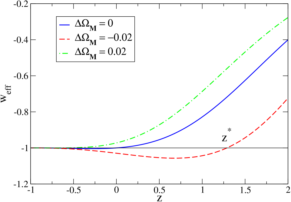
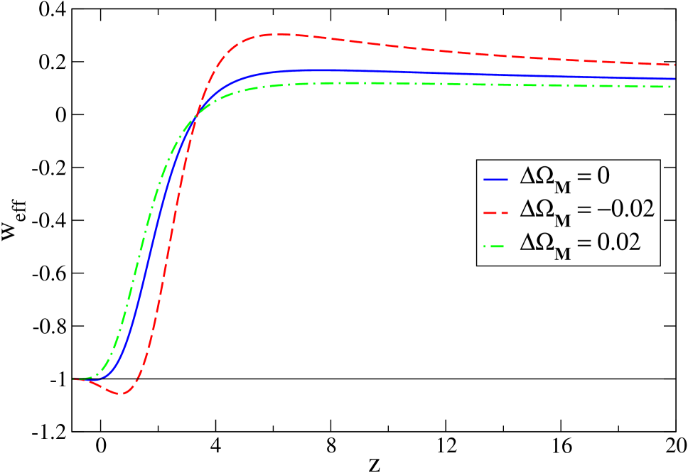
(a)	(b)

Figure 1: (a) Numerical analysis of the effective EOS parameter $w_{\rm eff}$, Eq. (23), as a function of the redshift for fixed $\nu=-\nu_{0}<0$, and for various values of $\Delta\Omega_{M}$. The Universe is assumed to be spatially flat ($\Omega_{K}^{0}=0$) with the standard parameter choice $\Omega_{M}^{0}=0.3\,,\Omega_{\Lambda}^{0}=0.7$; (b) Extended $z$ range of the plot (a). We see that for $\Delta\Omega_{M}<0$ there exists a transition point $z^{*}$ near our recent past: namely, the one corresponding to the crossing of the CC barrier $w_{\rm eff}=-1$ by the lowest curve in the figures.

6 Conclusions

We have shown that a model with variable $\Lambda$ (and possibly of $G$) generally leads to a non-trivial effective EOS, thus mimicking a canonical dynamical DE model (i.e. one with conserved DE density). That EOS can effectively appear as quintessence and even as phantom energy. Moreover, we have proven that there always exists a transition point $z^{*}$ near $z=0$ where $w_{\rm eff}(z^{*})=-1$. If this point lies in our recent past (as illustrated in Fig. 1a) there could have been a recent transition into an (effective) phantom regime $w_{\rm eff}(z)<-1$, as suggested by several analysis of the data. If, however, experiments would unambiguously indicate $w_{\rm eff}(z)>-1$ we could equally well interpret this in our framework, for $z^{*}$ could just be in our immediate future. We conclude that variable $(\rho_{\Lambda},G)$ models may account for the observed evolution of the DE, without need of invoking any combination of fundamental quintessence and phantom fields. The eventual determination of an empirical EOS for the DE in the next generation of precision cosmology experiments should keep in mind this possibility.

Acknowledgements. This work has been supported in part by MEC and FEDER under project 2004-04582-C02-01, and also by DURSI Generalitat de Catalunya under project 2005SGR00564. The work of HS is financed by the Secretaria de Estado de Universidades e Investigación of the Ministerio de Educación y Ciencia of Spain. HS thanks the Dep. ECM of the Univ. of Barcelona for the hospitality.

References

References

- [1] A.G. Riess et al., Astronom. J. 116 (1998) 1009; S. Perlmutter et al., Astrophys. J. 517 (1999) 565; R. A. Knop et al., Astrophys. J. 598 (2003) 102; A.G. Riess et al. Astrophys. J. 607 (2004) 665.
- [2] WMAP Collab.: http://map.gsfc.nasa.gov/; M. Tegmark et al, Phys. Rev. D69 (2004) 103501.
- [3] C. Deffayet, G.R. Dvali, G. Gabadadze, Phys. Rev. D65 (2002) 044023.
- [4] E.V. Linder, Phys. Rev. D 70 (2004) 023511; S. Hannestad, E. Mortsell, JCAP 0409 (2004) 001.
- [5] S. Weinberg, Rev. Mod. Phys. 61 (1989) 1; V. Sahni, A. A. Starobinsky, Int. J. of Mod. Phys. 9 (2000) 373; S.M. Carroll, Living Rev. Rel. 4 (2001) 1; J. Solà, Nucl. Phys. Proc. Suppl. 95 (2001) 29; T. Padmanabhan, Phys. Rep. 380 (2003) 235.
- [6] T. Padmanabhan, Curr. Sci. 88 (2005) 1057, astro-ph/0411044.
- [7] R.R. Caldwell, R. Dave, P.J. Steinhardt, Phys. Rev. Lett. 80 (1998) 1582; C. Wetterich, Nucl. Phys. B302 (1988) 668; B. Ratra, P.J.E. Peebles, Phys. Rev. D37 (1988) 3406; For a review, see e.g. P.J.E. Peebles, B. Ratra, Rev. Mod. Phys. 75 (2003) 559.
- [8] R.R. Caldwell, Phys. Lett. B545 (2002) 23; A. Melchiorri, L. Mersini, C.J. Odman, M. Trodden, Phys. Rev. D68 (2003) 043509; H. Štefančić, Phys. Lett. B586 (2004) 5; ibid. Eur. Phys. J. C36 (2004) 523; S. Nojiri, S.D. Odintsov, Phys. Rev. D70 (2004) 103522; S. Capozziello, S. Nojiri, S.D. Odintsov, hep-th/0512118; J.S. Alcaniz, H. Stefancic, astro-ph/0512622.
- [9] A. Yu. Kamenshchik, U. Moschella, V. Pasquier, Phys. Lett. B511 (2001) 265, gr-qc/0103004; N. Bilic, G.B. Tupper, R.D. Viollier, Phys. Lett. B535 (2002) 17.
- [10] A.D. Dolgov, in: The very Early Universe, Ed. G. Gibbons, S.W. Hawking, S.T. Tiklos (Cambridge U., 1982); F. Wilczek, Phys. Rep. 104 (1984) 143; L. Abbot, Phys. Lett. B 150 (1985) 427.
- [11] R.D. Peccei, J. Solà, C. Wetterich, Phys. Lett. B195 (1987) 183; S.M. Barr, Phys. Rev. D 36 (1987) 1691; J. Solà, Phys. Lett. B228 (1989) 317; ibid., Int. J. of Mod. Phys. 5 (1990) 4225.
- [12] I.L. Shapiro, J. Solà, JHEP 0202 (2002) 006, hep-th/0012227; I.L. Shapiro, J. Solà, Phys. Lett. B475 (2000) 236, hep-ph/9910462.
- [13] A. Babic, B. Guberina, R. Horvat, H. Štefančić, Phys. Rev. D65 (2002) 085002; B. Guberina, R. Horvat, H. Štefančić, Phys. Rev. D67 (2003) 083001.
- [14] A. Bonanno, M. Reuter, Phys. Rev. D65 (2002) 043508; E. Bentivegna, A. Bonanno, M. Reuter, JCAP 0401 (2004) 001; F. Bauer, Class.Quant.Grav. 22 (2005) 3533; ibid. gr-qc/0512007.
- [15] M. Reuter, C. Wetterich, Phys. Lett. B188 (1987) 38; K. Freese, F. C. Adams, J. A. Frieman, E. Mottola, Nucl. Phys. B287 (1987) 797; J.C. Carvalho, J.A.S. Lima, I.Waga, Phys. Rev. D46 (1992) 2404; J.M. Overduin, F. I. Cooperstock, Phys. Rev. D58 (1998) 043506.
- [16] I.L. Shapiro, J. Solà, C. España-Bonet, P. Ruiz-Lapuente, Phys. Lett. B574 (2003) 149; ibid. JCAP 0402 (2004) 006; I.L. Shapiro, J. Solà, Nucl. Phys. Proc. Supp. 127 (2004) 71.
- [17] I.L. Shapiro, J. Solà, H. Štefančić, JCAP 0501 (2005) 012.
- [18] A. Vikman, Phys. Rev. D71 (2005) 023515; B. Feng, X-L. Wang, X-M. Zhang, Phys. Lett. B607 (2005) 35; H. Štefančić, Phys. Rev. D71 (2005) 124036.
- [19] J. Solà, H. Štefančić, Phys. Lett. B624 (2005) 147, astro-ph/0505133; J. Solà, H. Štefančić, astro-ph/0507110 (Mod. Phys. Lett. A, in press); J. Solà, gr-qc/0512030.
- [20] R.R. Caldwell, M. Kamionkowski, N.N. Weinberg, Phys. Rev. Lett. 91 (2003) 071301; U. Alam, V. Sahni, A.A. Starobinsky, JCAP 0406 (2004) 008; H.K. Jassal, J.S. Bagla, T. Padmanabhan, Mon. Not. Roy. Astron. Soc. Letters 356 (2005) L11-L16.