Coupling of Radial and Axial non-Radial Oscillations of Compact Stars: Gravitational Waves from first-order Differential Rotation

Abstract

We investigate the non-linear coupling between radial and non-radial oscillations of static spherically symmetric neutron stars as a possible mechanism for the generation of gravitational waves that may lead to observable signatures. In this paper we concentrate on the axial sector of the non-radial perturbations. By using a multi-parameter perturbative framework we introduce a complete description of the non-linear coupling between radial and axial non-radial oscillations; we study the gauge invariant character of the associated perturbative variables and develop a computational scheme to evolve the non-linear coupling perturbations in the time domain. We present results of simulations corresponding to different physical situations and discuss the dynamical behaviour of this non-linear coupling. Of particular interest is the occurrence of signal amplifications in the form of resonance phenomena when a frequency associated with the radial pulsations is close to a frequency associated with one of the axial $w$-modes of the star. Finally, we mention possible extensions of this work and improvements towards more astrophysically motivated scenarios.

I Introduction

Gravitational wave astronomy is currently developing as a new way of studying the cosmos, with a number of different experiments starting operating or being developed: earth-based interferometers (LIGO lig , VIRGO vir , GEO600 geo and TAMA tam ), resonant bars (EXPLORER, AURIGA, NAUTILUS, ALLEGRO and NIOBE; see bar ) and spheres such as MiniGRAIL min , as well as the laser interferometer space antenna LISA lis . The scientific success of these detectors in producing new physical and astrophysical knowledge depends on the amount of a priori available theoretical understanding about the different sources of gravitational waves. It is then of outmost importance to have good theoretical descriptions of the systems that are likely to be observed by the ongoing gravitational-wave experiments.

Due to the weak character of the gravitational interactions there is only a few number of systems that can generate gravitational waves detectable for the experiments just mentioned. In general, the dynamics of these systems involves strong gravitational fields that need to be described, using different levels of approximations, by general relativity. This is the case in the modeling of compact objects such as neutron stars and supernovæ core collapse, where non-linearity plays a role in the dynamics. For these systems, relativistic perturbation theory is an excellent approach. The linear theory has been used for a long time to study their oscillations and instabilities Andersson (2003); Kokkotas and Ruoff (2002). However, we know relatively little about non-linear dynamical effects (mainly due to numerical studies Sperhake et al. (2001); Schenk et al. (2002); Morsink (2002); Lindblom et al. (2002); Arras et al. (2003); Font et al. (2002); Stergioulas et al. (2004); Dimmelmeier et al. (2005)). Despite the fact that strong non-linear effects require a fully non-perturbative approach, it is reasonable to expect that there are interesting physical phenomena that only involve a mild non-linearity for which a second-order treatment should be perfectly suited. In this sense, a non-linear perturbative approach is therefore timely and may lead to a better understanding of the mechanisms of generation of gravitational waves.

An interesting scenario to study is a neutron star which is oscillating radially and non-radially. At first order radial oscillations of a spherical star don’t emit per se any gravitational waves, but they can drive and possibly amplify non-radial oscillations and then produce gravitational radiation to a significant level. In addition one may expect the appearance of non-linear harmonics, which may also come out at lower frequencies than the linear modes Zanotti et al. (2004); Dimmelmeier et al. (2005), where the Earth-based laser interferometers have a higher sensitivity. An additional motivation is that there are a number of studies aiming at investigating if non-radial oscillations of stars can be excited by external sources (see e.g. Gualtieri et al. (2001); Poisson (1993)). However, our idea is to investigate whether non-radial oscillations can be driven or even amplified through coupling by an internal radial oscillation, regardless of the presence of an external source. These non-linear processes can occur, for instance, in a proto-neutron star that is still pulsating. A mainly radial pulsation could for example drive the non-radial oscillations, either naturally present, or excited through fall-back accretion.

In recent papers Bruni et al. (2003); Sopuerta et al. (2004) a non-linear multi-parameter perturbative formalism has been developed, which can be applied to the study of the non-linear dynamics of the oscillations of neutron stars, as shown in Passamonti et al. (2005) where it has been further developed to study a particular second-order effect: the coupling of radial and non-radial first order perturbations of a compact spherical star. One of the main ideas behind this work is that it is very convenient to treat the two sets of perturbations, radial and non-radial, as separately parametrized and then to study, at the next perturbative order, the way in which they couple, which corresponds to a particular sector of the second-order perturbations, the one formed by the product of radial and non-radial perturbations. In Passamonti et al. (2005), the equations describing the coupling were obtained for the case of polar non-radial perturbations and gauge-invariant variables were also found (having fixed the gauge for the radial ones for simplicity).

In this paper, we extend this study to the case of axial perturbations. At first order, axial perturbations are decoupled from fluid perturbations, but at the next perturbative order, the terms describing the coupling are driven by the radial pulsations. Here we discuss the results of simulations in the time domain that show how the coupling mechanism works and under which conditions we may have a situation in which this coupling produces amplifications due to resonant phenomena.

The plan of this paper is the following: In Section II we describe the perturbative framework we use in this work. In Section III we introduce all the necessary ingredients required by the perturbative scheme in order to study the coupling of radial and axial non-radial oscillations of neutron stars. In Section IV we describe the structure of the computational framework we have implemented to solve the perturbative equations in the time domain. In particular, we discuss in detail the construction of initial data and the numerical treatment of the boundary conditions. In Section V we present the results of our simulations for two different physical scenarios: (i) the scattering of a gravitational wave packet by a differentially rotating star, and (ii) the non-linear coupling in a differentially rotating and radially oscillating compact star. In particular we discuss the appearance of amplifications due to resonances of the system. We conclude in Section VI, where we summarize the main results of this paper and discuss potential extensions of the approach we have used. In the Appendices we give some proofs of the gauge invariance character of some of the perturbative quantities (Appendix A), expressions for the source terms in the perturbative equations describing the coupling (Appendix B), and the equations for radial perturbations in terms of the tortoise fluid coordinate (Appendix C).

Throughout this work we use the following conventions: We use Greek letters to denote spacetime indices; capital Latin letters for indices in the time-radial part of the metric; lower-case Latin indices for the spherical sector of the metric. We use physical units in which $8\pi G=c=1\,$.

II Perturbative Framework

In order to investigate the effects of the coupling of linear axial perturbations and first order radial oscillations we use a general two-parameter framework recently developed Bruni et al. (2003); Sopuerta et al. (2004). In essence, this consists of separately parametrizing the radial and non radial oscillations. We have presented the formalism for the coupling between radial and polar non-radial perturbations in Passamonti et al. (2005). In this paper we develop and apply the formalism to study the coupling arising from axial perturbations, following the same general lines. In the following we recall the general two-parameter framework. However, to fix the ideas, we will refer explicitly to its application to the case of stellar oscillations.

The physical spacetime of the oscillating star we consider is represented as a non-linear perturbation of a static spherical background stellar model, with metric $\mbox{\boldmath$\mbox{\bf g}$}^{(0,0)}\,$. The expansion of the physical metric g around this background has the following form:

$$\mbox{g}_{\alpha\beta}=\mbox{g}^{(0,0)}_{\alpha\beta}+\lambda\,\mbox{g}^{(1,0)}_{\alpha\beta}+\epsilon\,\mbox{g}^{(0,1)}_{\alpha\beta}+\lambda\epsilon\,\mbox{g}^{(1,1)}_{\alpha\beta}+O(\lambda^{2},\epsilon^{2})\,,$$ (1)

where $\lambda$ and $\epsilon$ are the expansion parameters associated with radial and non-radial perturbations respectively. We use superscripts $(I,J)$ to denote perturbations of order $\lambda^{I}\epsilon^{J}$. Therefore, the terms $\mbox{\boldmath$\mbox{\bf g}$}^{(1,0)}$ and $\mbox{\boldmath$\mbox{\bf g}$}^{(0,1)}$ in (1) represent, respectively, first-order radial and non-radial perturbations, while $\mbox{\boldmath$\mbox{\bf g}$}^{(1,1)}$ is the non-linear contribution due to their coupling. This is the quantity we are interested in this paper, while we will neglect the self-coupling terms of order $\lambda^{2}$ and $\epsilon^{2}$.

Any physical quantity can be expanded as the metric in (1). In particular, the energy-momentum tensor has the expansion:

$$T_{\alpha\beta}=T^{(0,0)}_{\alpha\beta}+\lambda T^{(1,0)}_{\alpha\beta}+\epsilon T^{(0,1)}_{\alpha\beta}+\lambda\epsilon T^{(1,1)}_{\alpha\beta}+O(\lambda^{2},\epsilon^{2})\,.$$ (2)

Let us now analyze the structure of the field equations

$$\mbox{\boldmath$E$}\left[\,\mbox{\bf g}\,,\mbox{\boldmath$\psi$}_{A}\,\right]=\mbox{\boldmath$G$}\left[\,\mbox{\bf g}\,\right]-\mbox{\boldmath$T$}\left[\,\mbox{\bf g}\,,\mbox{\boldmath$\psi$}_{A}\,\right]=0$$ (3)

arising from the perturbative expansion (see e.g. Wald (1984)). Here $G$ denotes the Einstein tensor, $T$ the energy-momentum tensor and $\mbox{\boldmath$\psi$}_{A}$ (A=$1,\dots$) the matter variables. Introducing (1) and (2) into Eq. (3) we obtain the perturbative equations at each order:

$$\mbox{\boldmath$E$}\left[\,\mbox{\bf g}\,,\mbox{\boldmath$\psi$}_{A}\,\right]=\mbox{\boldmath$E$}^{(0,0)}\left[\,\mbox{\boldmath$\mbox{\bf g}$}^{(0,0)}\,,\mbox{\boldmath$\psi$}_{A}^{(0,0)}\,\right]+\lambda\mbox{\boldmath$E$}^{(1,0)}\left[\,\mbox{\boldmath$\mbox{\bf g}$}^{(1,0)}\,,\mbox{\boldmath$\psi$}_{A}^{(1,0)}\,\right]+\epsilon\mbox{\boldmath$E$}^{(0,1)}\left[\,\mbox{\boldmath$\mbox{\bf g}$}^{(0,1)}\,,\mbox{\boldmath$\psi$}_{A}^{(0,1)}\,\right]$$

$$\quad+\lambda\epsilon\mbox{\boldmath$E$}^{(1,1)}\left[\,\mbox{\boldmath$\mbox{\bf g}$}^{(1,1)}\,,\mbox{\boldmath$\psi$}_{A}^{(1,1)}\;\left|\;\mbox{\boldmath$\mbox{\bf g}$}^{(1,0)}\otimes\mbox{\boldmath$\mbox{\bf g}$}^{(0,1)}\,,\mbox{\boldmath$\psi$}_{A}^{(1,0)}\otimes\mbox{\boldmath$\psi$}_{A}^{(0,1)}\,,\mbox{\boldmath$\mbox{\bf g}$}^{(1,0)}\otimes\mbox{\boldmath$\psi$}_{A}^{(0,1)}\,,\mbox{\boldmath$\psi$}_{A}^{(1,0)}\otimes\mbox{\boldmath$\mbox{\bf g}$}^{(0,1)}\,\right]+O(\lambda^{2},\epsilon^{2})=0\,.\right.$$ (4)

This equation has to be satisfied for arbitrary values of the expansion parameters, therefore each perturbative term must vanish independently. This naturally gives rise to an iterative scheme, where at each non-linear order one has to solve inhomogeneous equations with source terms containing the solutions of the lower order equations.

The lowest order in (4), $\mbox{\boldmath$E$}^{(0,0)}=0$, gives the equations for the background, in our case the Tolman-Oppenheimer-Volkoff (TOV) equations. The other terms $\mbox{\boldmath$E$}^{(I,J)}=0$ represent the perturbative equations of order $\lambda^{I}\epsilon^{J}\,$. The structure of the operators $\mbox{\boldmath$E$}^{(I,J)}$, with $(I,J)\neq(0,0)$, is such that they act linearly on every term specified between the square brackets, while they are non-linear functions of the background quantities $\mbox{\bf g}^{(0,0)}$ and $\mbox{\boldmath$\psi$}_{A}^{(0,0)}$. At first order in $\lambda$, we obtain the equations describing the radial perturbations of the TOV background, $\mbox{\boldmath$E$}^{(1,0)}=0$, whereas axial non-radial perturbations come from the first-order terms in $\epsilon$:

$$\mbox{\boldmath$E$}^{(0,1)}\left[\,\mbox{\boldmath$\mbox{\bf g}$}^{(0,1)}\,,\mbox{\boldmath$\psi$}_{A}^{(0,1)}\,\right]=0\,.$$ (5)

Finally, the equations of order $\lambda\epsilon$ describe the radial non-radial coupling:

$$\mbox{\boldmath$E$}^{(1,1)}\biggl{[}\,\mbox{\boldmath$\mbox{\bf g}$}^{(1,1)}\,,\mbox{\boldmath$\psi$}_{A}^{(1,1)}~{}\left|~{}\mbox{\boldmath$\mbox{\bf g}$}^{(1,0)}\otimes\mbox{\boldmath$\mbox{\bf g}$}^{(0,1)}\,,\mbox{\boldmath$\psi$}_{A}^{(1,0)}\otimes\mbox{\boldmath$\psi$}_{A}^{(0,1)}\,,\right.$$

$$~{}~{}~{}~{}~{}~{}~{}~{}~{}~{}\mbox{\boldmath$\mbox{\bf g}$}^{(1,0)}\otimes\mbox{\boldmath$\psi$}_{A}^{(0,1)}\,,\mbox{\boldmath$\psi$}_{A}^{(1,0)}\otimes\mbox{\boldmath$\mbox{\bf g}$}^{(0,1)}\,\biggr{]}=0\,,$$ (6)

where the vertical bar separates the unknowns of order $\lambda\epsilon$ from the quantities computed in the previous iteration of the perturbative scheme, which form the source terms of the equations.

In order to solve these equations, it is important to take into account that the operator $\mbox{\boldmath$E$}^{(1,1)}$ acts on $(\mbox{\boldmath$\mbox{\bf g}$}^{(1,1)}\,,\mbox{\boldmath$\psi$}_{A}^{(1,1)})$ in Eq. (6) in the same way as $\mbox{\boldmath$E$}^{(0,1)}$ acts on $(\mbox{\boldmath$\mbox{\bf g}$}^{(0,1)}\,,\mbox{\boldmath$\psi$}_{A}^{(0,1)})$ in Eq. (5). The reason is that both operators come from the linearization of the Einstein tensor operator acting on axial non-radial perturbations. Then, using the linearity of $\mbox{\boldmath$E$}^{(1,1)}$, we can define

$$\mbox{\boldmath$L$}_{\rm NR}\left[\,\cdot\,\right]\equiv\mbox{\boldmath$E$}^{(1,1)}\left[\,\cdot\,|\,\mbox{\boldmath$0$}\,\right]=\mbox{\boldmath$E$}^{(0,1)}\left[\,\cdot\,\right]\,,$$ (7)

as the axial non-radial perturbation operator. Hence, equation (6) can be written in the form:

$$\mbox{\boldmath$L$}_{\rm NR}\left[\,\mbox{\boldmath$\mbox{\bf g}$}^{(1,1)}\,,\mbox{\boldmath$\psi$}_{A}^{(1,1)}\,\right]=\mbox{\boldmath$S$}\biggl{[}\mbox{\boldmath$\mbox{\bf g}$}^{(1,0)}\otimes\mbox{\boldmath$\mbox{\bf g}$}^{(0,1)}\,,$$

$$\mbox{\boldmath$\psi$}_{A}^{(1,0)}\otimes\mbox{\boldmath$\psi$}_{A}^{(0,1)}\,,\mbox{\boldmath$\mbox{\bf g}$}^{(1,0)}\otimes\mbox{\boldmath$\psi$}_{A}^{(0,1)}\,,\mbox{\boldmath$\psi$}_{A}^{(1,0)}\otimes\mbox{\boldmath$\mbox{\bf g}$}^{(0,1)}\,\biggr{]}\,.$$ (8)

This particular structure of the equations is very important in solving them by using time-domain numerical methods. Indeed, we can easily extend a numerical code that solves the equations for first-order axial non-radial perturbations simply by adding the source terms on the right-hand side of (8). Later on we will discuss additional advantages of this structure.

III Perturbative scheme for stellar oscillations

In this section we introduce the basic ingredients needed to study the coupling of radial and axial perturbations of relativistic stars: the background description (Sec. III.1), the first-order radial and axial perturbations (Secs. III.2 and III.3), and finally the equations describing the coupling of the first-order perturbations (Sec. III.4). To simplify our expressions we denote the background quantities with an overbar, e.g. $\bar{\mbox{g}}_{\alpha\beta}=\mbox{g}^{(0,0)}_{\alpha\beta}$ and $\bar{T}_{\alpha\beta}=T^{(0,0)}_{\alpha\beta}\,$.

III.1 The static spherically-symmetric background

The background is an equilibrium configuration described by a static spherically-symmetric metric (see, e.g., Misner et al. (1973)), a TOV model. The line-element is:

$$\bar{\mbox{g}}_{\alpha\beta}dx^{\alpha}dx^{\beta}=-e^{2\Phi}dt^{2}+e^{2\Lambda}dr^{2}+r^{2}(d\theta^{2}+\sin^{2}\theta d\phi^{2})\,,$$ (9)

where $\Phi$ and $\Lambda$ are functions of $r$ only. This is a solution of Einstein’s equations with a perfect-fluid energy-momentum tensor

$$\bar{T}_{\alpha\beta}=(\bar{\rho}+\bar{p})\,\bar{u}_{\alpha}\bar{u}_{\beta}+\bar{p}\,\bar{\mbox{g}}_{\alpha\beta}\,,$$ (10)

where the four-velocity of the fluid is $\bar{u}_{\alpha}=\left(-e^{\Phi},0,0,0\right)$, and in general $\rho$ and $p$ denote the energy density and the pressure. The mass function $m(r)$ is introduced through the metric function $\Lambda$: $e^{-2\Lambda(r)}=1-2m(r)/r\,$. The TOV equations of stellar equilibrium read:

$$\Phi_{,r} = \frac{m+4\pi r^{3}\bar{p}}{r(r-2m)}=-\frac{\bar{p}_{,r}}{\bar{\rho}+\bar{p}}\,,$$ (11)

$$m_{,r} = 4\pi r^{2}\bar{\rho}\,.$$ (12)

Specifying the Equation of State (EoS) of the stellar equilibrium configuration yields a 1-parameter family of solutions of the equations (11,12), which is typically parametrized by the value of the central density $\bar{\rho}_{c}=\bar{\rho}(r\!=\!0)\,$. Here we consider a configuration described by an adiabatic, barotropic EoS generalization of the Newtonian polytropic EoS:

$$\bar{p}=K\bar{\rho}^{\Gamma}\,,$$ (13)

where $K$ is a constant and $\Gamma$ the polytropic index. In particular, we take $K\!=\!100$ km², $\Gamma\!=\!2\,$, $\bar{\rho}_{c}=3\times 10^{15}$ g/cm³. These values yield a stellar configuration with mass $M=1.26M_{\odot}$ and radius $R=8.86$ km. We denote by $\bar{c}_{s}=(d{\bar{p}}/d{\bar{\rho}})^{1/2}$ the speed of sound.

III.2 Radial Perturbations of the TOV Model

Radial perturbations (first investigated by S. Chandrasekhar Chandrasekhar (1964, 1964); see also Kokkotas and Ruoff (2001)), by definition, preserve the spherical symmetry of the TOV background. They can be completely described in terms of the Lagrangian displacement of a fluid element around its equilibrium position. Alternatively, in the radial gauge, they can be written in terms of two metric functions:

$$g^{(1,0)}_{\alpha\beta}dx^{\alpha}dx^{\beta} = e^{2\Phi}(rS^{(1,0)}-2\eta^{(1,0)})dt^{2}$$ (14)

$$+ re^{2\Lambda}S^{(1,0)}dr^{2}\,.$$

The radial perturbations of the fluid variables in this gauge are:

$$u_{\alpha}^{(1,0)}dx^{\alpha} = e^{\Phi}(\textstyle{\frac{r}{2}}S^{(1,0)}-\eta^{(1,0)})dt+e^{\Lambda}\gamma^{(1,0)}dr\ ,$$ (15)

$$\delta\rho^{(1,0)} = \bar{\rho}\,\omega^{(1,0)}\ ,$$ (16)

$$\delta p^{(1,0)} = \bar{c}_{s}^{2}\bar{\rho}\,\omega^{(1,0)}\,.$$ (17)

To simplify the equations we use the following perturbative quantities: metric variables: the metric perturbations $\eta^{(1,0)}$ and $S^{(1,0)}\,$; matter variables: the fluid velocity perturbation $\gamma^{(1,0)}$ and the enthalpy perturbation, which is related to the density perturbations through the relation:

$$H^{(1,0)}=\frac{\bar{c}_{s}^{2}\bar{\rho}}{\bar{\rho}+\bar{p}}\omega^{(1,0)}\,.$$ (18)

The dynamics of radial pulsations is then governed by the following system of PDEs:

$$H_{,t}^{(1,0)} = -\bar{c}_{s}^{2}e^{\Phi-\Lambda}\left\{\gamma^{(1,0)}_{,r}+e^{2\Lambda}\left[\left(1-\frac{1}{\bar{c}_{s}^{2}}\right)\left(4\pi r\bar{p}+\frac{m}{r^{2}}\right)+\frac{2}{r}e^{-2\Lambda}-4\pi(\bar{\rho}+\bar{p})\right]\gamma^{(1,0)}\right\}\,,$$ (19)

$$\gamma_{,t}^{(1,0)} = -e^{\Phi+\Lambda}\left\{e^{-2\Lambda}H^{(1,0)}_{,r}+4\pi r(\bar{\rho}+\bar{p})H^{(1,0)}+\frac{1}{2}\left(1+8\pi r^{2}\bar{p}\right)S^{(1,0)}\right\}\,,$$ (20)

$$S_{,t}^{(1,0)} = -8\pi(\bar{\rho}+\bar{p})e^{\Phi+\Lambda}\gamma^{(1,0)}\,,$$ (21)

which was derived in Passamonti et al. (2005) using the formalism of Gerlach and Sengupta (1979, 1980); Martín-García and Gundlach (1999); Gundlach and Martín-García (2000); Martín-García and Gundlach (2001) (see Section III.3 below). A similar system was obtained in Ruoff (2000) using the well-known ADM 3+1 formalism Arnowitt et al. (1962); York (1979). Having solved the above system, the metric variable $\eta^{(1,0)}$ can then be obtained from the following relation

$$\eta^{(1,0)}_{,r}=4\pi r(\bar{\rho}+\bar{p})\left[rS^{(1,0)}+\left(1+\frac{1}{\bar{c}^{2}_{s}}\right)H^{(1,0)}\right]e^{2\Lambda}\,.$$ (22)

Finally, our variables have to satisfy the Hamiltonian constraint, which takes the following form

$$S^{(1,0)}_{,r}=e^{2\Lambda}\biggl{[}\left(8\pi r\bar{\rho}-\frac{2}{r}+\frac{2m}{r^{2}}\right)S^{(1,0)}+8\pi\frac{\bar{\rho}+\bar{p}}{\bar{c}_{s}^{2}}H^{(1,0)}\biggr{]}\,.$$ (23)

Boundary conditions must be fixed at the center and at the stellar surface $r\!=\!R$. The vanishing at the surface of the first-order Lagrangian pressure perturbation, $\Delta p^{(1,0)}(R)=0$, leads to the following condition on $\gamma^{(1,0)}$ Passamonti et al. (2005):

$$(\bar{\rho}+\bar{p})\,\bar{c}^{2}_{s}(r^{2}e^{-\Lambda}\gamma^{(1,0)})_{,r}|_{r=R}=0\,.$$ (24)

The behaviour of $S^{(1,0)}$ and $H^{(1,0)}$ on the surface can be derived from the general evolution equations (19) and (21). In the radial gauge there is still a residual gauge degree of freedom, which can be used for setting to zero all the pure gauge perturbations of the vacuum external spacetime Martín-García and Gundlach (2001). For stellar models where the density vanishes on the stellar surface, this gauge choice induces also $S^{(1,0)}$ and $\eta^{(1,0)}$ to vanish on that surface Martín-García and Gundlach (2001). At $r=0$, regularity conditions imply

$$S^{(1,0)} = rS^{(1,0)}_{o}(t)+O(r^{3})\,,$$ (25)

$$\eta^{(1,0)} = \eta^{(1,0)}_{o}(t)+O(r^{2})\,,$$ (26)

$$H^{(1,0)} = H^{(1,0)}_{o}(t)+O(r^{2})\,,$$ (27)

$$\gamma^{(1,0)} = r\gamma^{(1,0)}_{o}(t)+O(r^{3})\,.$$ (28)

III.3 Axial Perturbations of the TOV Model

Axial oscillations of a static star were first investigated by Thorne and Campolattaro Thorne and Campolattaro (1967, 1968); Campolattaro and Thorne (1970), and have been the subject of many subsequent studies (see, e.g. Chandrasekhar and Ferrari (1991); Andersson and Kokkotas (1996)).

Non-radial perturbations are nicely described in the formalism introduced by Gerlach and Sengupta Gerlach and Sengupta (1979, 1980) and further developed by Gundlach and Martín-García Martín-García and Gundlach (1999); Gundlach and Martín-García (2000); Martín-García and Gundlach (2001) (which we denote as GSGM formalism). This was originally introduced to study first order perturbations of a general time-dependent spherically symmetric stellar background. In particular we can apply it to our case, where the background is the static TOV metric.

III.3.1 Summary of the GSGM formalism for axial perturbations

The key point in the GSGM formalism is the fact that the background manifold is a warped product $M^{2}\times S^{2}$, where $S^{2}$ denotes the 2-sphere and $M^{2}$ is a two-dimensional Lorentzian manifold. The metric can be written as the semidirect product of a general Lorentzian metric on $M^{2}$, $\bar{g}_{AB}$, and the unit curvature metric $\gamma_{ab}$ on $S^{2}$:

$$\bar{\mbox{g}}_{\alpha\beta}=\left(\begin{array}[]{cc}\bar{g}_{AB}&0\\ 0&r^{2}\gamma_{ab}\end{array}\right)\,.$$ (29)

Hereafter $x^{A}$ denote the coordinates on $M^{2}$, $x^{a}$ the coordinates on $S^{2}$ and $r=r(x^{A})$ is a function on $M^{2}$ that coincides with the invariantly defined radial (area) coordinate of spherically-symmetric spacetime. A vertical bar is used to denote the covariant derivative on $M^{2}$ and a semicolon to denote that on $S^{2}$. The metrics are covariantly conserved, i.e. $\bar{g}_{AB|C}=\gamma_{ab:c}=0$ . One can introduce the completely antisymmetric covariant unit tensors on $M^{2}$ and on $S^{2}$, $\bar{\epsilon}_{AB}$ and $\epsilon_{ab}$ respectively.

The energy-momentum tensor has the same block diagonal structure as the metric:

$$\bar{T}_{\alpha\beta}=\textrm{diag}\left(\bar{\rho}\bar{u}_{A}\bar{u}_{B}+\bar{p}\bar{n}_{A}\bar{n}_{B}\,,\,r^{2}\bar{p}\,\gamma_{ab}\right)\,,$$ (30)

where $\bar{u}_{A}$ are the non-zero components of the fluid velocity, $\bar{u}_{\alpha}=(\bar{u}_{A},0)\,$, and $\bar{n}_{A}$ is a unit spacelike vector given by

$$\bar{n}_{A}=-\bar{\epsilon}_{AB}\bar{u}^{B}~{}~{}\Rightarrow~{}~{}\bar{n}_{A}\bar{u}^{A}=0\,.$$ (31)

Here we will focus on the axial non-radial perturbations (see Passamonti et al. (2005) for the polar ones). The metric and energy-momentum axial perturbations can be expanded in terms of the vector and tensor axial (or odd-parity) spherical harmonics

$$S^{lm}_{a}=\epsilon_{a}{}^{b}Y^{lm}_{:b}\,,~{}~{}~{}S^{lm}_{ab}=S^{lm}_{a:b}+S^{lm}_{b:a}\,,$$ (32)

where $Y^{lm}$ are the scalar spherical harmonics, in the following form

$$g^{(0,1)}_{\alpha\beta} = \left(\begin{array}[]{cc}0&h_{A}^{lm}\,S^{lm}_{a}\\[5.69054pt] h_{A}^{lm}\,S^{lm}_{a}&h^{lm}S^{lm}_{ab}\end{array}\right)$$ (35)

$$T^{(0,1)}_{\alpha\beta} = \left(\begin{array}[]{cc}0&\delta t_{A}^{lm}\,S^{lm}_{a}\\[5.69054pt] \delta t_{A}^{lm}\,S^{lm}_{a}&\delta t^{lm}S^{lm}_{ab}\end{array}\right),$$ (38)

where $h_{A}^{lm}\,$ $h^{lm}\,$, $\delta t_{A}^{lm}\,$, and $\delta t^{lm}$ are functions of $t$ and $r$ only. To simplify the notation, in the following we drop the harmonic indices $(l,m)$. As shown in Gerlach and Sengupta (1979, 1980), a complete set of axial gauge-invariant quantities is obtained by taking the following combinations of $h_{A}\,$, $h\,$, $\delta t_{A}\,$, and $\delta t\,$:

$$k_{A} = h_{A}-h_{\mid A}+2h\bar{v}_{A}\,,$$ (39)

$$L_{A} = \delta t_{A}-\bar{p}\,h_{A}\,,$$ (40)

$$L = \delta t-\bar{p}\,h\,,$$ (41)

where $k_{A}$ and $L_{A}$ are defined for $l\geq 1\,,$ $L$ is defined for $l\geq 2$, and $\bar{v}_{A}=r^{-1}r_{|A}\,$. The only axial fluid perturbation function arises from the expansion of the fluid velocity

$$u^{(0,1)}_{\alpha}=\left(0\,,\beta S_{a}\right)\,,$$ (42)

where $\beta$ is a gauge invariant variable. As it has been shown in Gundlach and Martín-García (2000), for a perfect fluid the energy-momentum gauge-invariant quantities take the form

$$L_{A}=(\bar{\rho}+\bar{p})\beta\bar{u}_{A}\,,\qquad L=0\,.$$ (43)

Then, the equations for the perturbations can be decoupled in terms of the following quantities Gerlach and Sengupta (1979, 1980)

$$\Psi=r^{3}\,\bar{\epsilon}^{AB}\left(r^{-2}k_{A}\right)_{\mid B}\,,~{}~{}\hat{\beta}=(\bar{\rho}+\bar{p})\beta$$ (44)

and their expressions are

$$\left[\frac{(r\Psi)_{\mid A}}{r^{2}}\right]^{|A}-\frac{(l-1)(l+2)}{r^{3}}\Psi=-16\pi\bar{\epsilon}^{AB}(\hat{\beta}\bar{u}_{A})_{\mid B}\,,$$ (45)

$$u^{A}{\hat{\beta}}_{\mid A}+(\bar{\mu}+2\bar{U})\hat{\beta}=0\,,$$ (46)

where the background quantities $\bar{\mu}$ and $\bar{U}$ are

$$\bar{\mu}=\bar{u}^{A}_{\mid A}\,,~{}~{}\bar{U}=\bar{u}^{A}\bar{v}_{A}=r^{-1}\bar{u}^{A}r_{\mid A}\,.$$ (47)

We can solve these equations by prescribing initial data for $\hat{\beta}$ and $\Psi$ at a time $t_{o}$, that is, giving $(\Psi_{o},\dot{\Psi}_{o},\hat{\beta}_{o})\,$. Equation (46) is an equation for $\hat{\beta}$ only that can be solved independently from (45). Its solution is constant along the integral curves of $\bar{u}^{A}$ (see Gundlach and Martín-García (2000)). With the solution of (46) we can solve the equation (45) for $\Psi\,$, where $\hat{\beta}$ enters only in the source term. Once we have solved equations (45,46) for $\Psi$ and $\hat{\beta}$, we can get the gauge-invariant metric perturbations $k_{A}$ by means of the following relation:

$$(l-1)(l+2)k_{A}=16\pi r^{2}\hat{\beta}\,\bar{u}_{A}-\bar{\epsilon}_{AB}(r\Psi)^{\mid B}\,.$$ (48)

We emphasize that the formalism as described so far applies to a general time dependent, spherically symmetric background spacetime.

III.3.2 GSGM formalism on the TOV background

In the case of our TOV static background, we have:

$$\bar{u}^{A}=(e^{-\Phi},0)\,,~{}~{}\bar{n}^{A}=(0,e^{-\Lambda})\,,~{}~{}\bar{\mu}=\bar{U}=0\,.$$ (49)

Then, the equations for the gauge-invariant axial perturbations $\Psi$ and $\hat{\beta}$ are

$$-\Psi_{,tt}+\Psi_{,r_{\ast}r_{\ast}}+e^{2\Phi}\left[4\pi(\bar{p}-\bar{\rho})+\frac{6M}{r^{3}}-\frac{l(l+1)}{r^{2}}\right]\Psi+16\pi re^{2\Phi+\Lambda}\left[e^{-2\Lambda}\hat{\beta}_{,r}+\left(4\pi r\bar{p}+\frac{M}{r^{2}}\right)\hat{\beta}\right]=0\,,$$ (50)

$$\hat{\beta}_{,t}=0\,,$$ (51)

where, to simplify the equations, we have introduced the tortoise coordinate

$$dr_{\ast}=e^{\Phi-\Lambda}dr\,.$$ (52)

Equation (51) tells us that $\hat{\beta}$ is not a dynamical variable and hence, at first order, is typically of no interest and can be consistently set to zero Thorne and Campolattaro (1967); Chandrasekhar and Ferrari (1991); Andersson and Kokkotas (1996). In this sense, it is said that first-order axial perturbations do not depend on the fluid motion.

As we discuss later in Section IV.2, $\beta_{lm}$ can however be taken to represent the harmonic component $lm$ of a first order differential rotation profile, and as such plays a very interesting role in the coupling, at order $\lambda\epsilon$, with radial oscillations.

Then, if we consider a non-vanishing $\hat{\beta}\,$, the general solution of (50) is the combination of (i) the solutions of the homogeneous associate equation that describes the only dynamical degrees of freedom of axial perturbations, i.e. the gravitational waves, and (ii) a particular (static) solution that is related to the dragging of inertial frames induced by a non-vanishing $\hat{\beta}$, as discussed in Thorne and Campolattaro (1967).

Outside the star, equation (50) reduces to the well-known Regge-Wheeler equation

$$-\Psi_{,tt}+\Psi_{,r_{\ast}r_{\ast}}-V_{l}(r)\Psi=0\,.$$ (53)

where

$$V_{l}(r)=\left(1-\frac{2M}{r}\right)\left(\frac{l(l+1)}{r^{2}}-\frac{6M}{r^{3}}\right)\,,$$ (54)

and $M$ is the gravitational mass of the TOV star. In (53), $r_{\ast}$ is the usual Regge-Wheeler tortoise coordinate $r_{\ast}\equiv r+2M\ln[r/(2M)-1]\,$. To complete the description of the first-order axial perturbations we need to discuss the boundary conditions at the origin, at the stellar surface, and at infinity. The requirement of regularity of the perturbations at the origin yields

$$\hat{\beta}\sim r^{l+1}\,,\qquad\Psi\sim r^{l+1}\,.$$ (55)

The matching conditions on the stellar surface imply the continuity of metric variable $\Psi\,$, of its time derivative, and of the following quantity Martín-García and Gundlach (2001):

$$e^{-\Lambda}\left(r^{-3}\Psi\right)_{,r}-16\pi r^{-2}\,\hat{\beta}\,.$$ (56)

In the case of a barotropic equation of state, the pressure and mass-energy density vanish on the surface, and the condition (56) reduces to the continuity of $\Psi_{,r}$. At infinity we can simply use Sommerfeld outgoing wave conditions.

The master function $\Psi$ is related to the emitted power in gravitational waves at infinity (see, e.g. Nagar and Rezzolla (2005)):

$$\frac{dE}{dt}=\sum_{l,m}P_{lm}=\frac{1}{16\pi}\sum_{l,m}\frac{l(l+1)}{(l-1)(l+2)}|\dot{{\Psi}}_{lm}|^{2}\,,$$ (57)

where we have explicitly restored the harmonic indices $(l,m)$ and the overdot denotes time differentiation with respect to the Schwarzschild coordinate time.

III.4 Non-linear Coupling between radial and non-radial perturbations

To derive the equations that describe the non-linear coupling between first-order radial and axial non-radial oscillations we are going to follow the procedure used in the polar case Passamonti et al. (2005). In brief, the idea is to obtain the equations for the coupling from the equations for the axial perturbations (45) and (46), by using the following formal perturbative expansion:

$$\mbox{g}_{\alpha\beta}=\mbox{g}^{(0)}_{\alpha\beta}+\epsilon\,\mbox{g}^{(1)}_{\alpha\beta}\,,$$ (58)

where $\mbox{g}^{(0)}_{\alpha\beta}$ is a time dependent background composed of our static TOV background with the radial oscillations, that is $\mbox{g}^{(0)}_{\alpha\beta}=\bar{\mbox{g}}_{\alpha\beta}+\lambda\mbox{g}_{\alpha\beta}^{(1,0)}\,$, and $\mbox{g}^{(1)}_{\alpha\beta}$ represents axial non-radial perturbations containing the first-order radial perturbations and the non-linear coupling terms, that is $\mbox{g}^{(1)}_{\alpha\beta}=\mbox{g}^{(0,1)}_{\alpha\beta}+\lambda\mbox{g}^{(1,1)}_{\alpha\beta}\,$. As we have already mentioned in Sec. II this is due to the fact that the first-order axial and the coupling perturbations have essentially the same structure and are governed by the same type of equations.

The metric and energy-momentum axial perturbation of order $(1,1)$ can be expanded in odd-parity spherical harmonics as in the first-order case [see equations (35), (38)]. To distinguish them we use superscripts $(I,J)$ denoting the perturbative order $\lambda^{I}\epsilon^{J}\,$. In this way, the $(0,1)$ metric and energy-momentum perturbations are denoted by $h_{A}^{(0,1)}\,$, $h^{(0,1)}\,$, $t_{A}^{(0,1)}\,$, and $t^{(0,1)}\,$; and the $(1,1)$ ones by $h_{A}^{(1,1)}\,$, $h^{(1,1)}\,$, $t_{A}^{(1,1)}\,$, and $t^{(1,1)}\,$. Likewise, the velocity perturbations of order $(1,1)$ are written as $u^{(1,1)}_{\alpha}=(0\,,\beta^{(1,1)}S_{a})\,$.

Then, the gauge-invariant quantities that we construct by using the ansatz of (58) are:

$$k_{A}^{(1,1)} = h_{A}^{(1,1)}-h^{(1,1)}_{\mid A}+2h^{(1,1)}\bar{v}_{A}\,,$$ (59)

$$L_{A}^{(1,1)} = \delta t_{A}^{(1,1)}-\bar{p}h_{A}^{(1,1)}-\bar{\rho}\bar{c}^{2}_{s}\omega^{(1,0)}h_{A}^{(0,1)}\,,$$ (60)

$$L^{(1,1)} = \delta t^{(1,1)}-\bar{p}h^{(1,1)}-\bar{\rho}\bar{c}^{2}_{s}\omega^{(1,0)}h^{(0,1)}\,.$$ (61)

Comparing expressions (59)-(61) with expressions (39)-(41) we notice that they differ because of the presence of the products of first-order perturbations in the $(1,1)$ perturbations in (60,61) (see also Passamonti et al. (2005)). The gauge invariance of the $(1,1)$ quantities (59)-(61) is shown in Appendix A.

We can also construct the coupling perturbations $\hat{\beta}^{(1,1)}$ and $\Psi^{(1,1)}$ in the same way as $\hat{\beta}^{(0,1)}=\hat{\beta}$ and $\Psi^{(0,1)}=\Psi$ in (44) (see Appendix A for more details). We find that they satisfy the following equations:

$$-\Psi^{(1,1)}_{,tt}+\Psi^{(1,1)}_{,r_{\ast}r_{\ast}}+e^{2\Phi}\left[4\pi(\bar{p}-\bar{\rho})+\frac{6M}{r^{3}}-\frac{l(l+1)}{r^{2}}\right]\Psi^{(1,1)}+16\pi re^{2\Phi+\Lambda}\left[e^{-2\Lambda}\hat{\beta}_{,r}^{(1,1)}+\left(4\pi r\bar{p}+\frac{M}{r^{2}}\right)\hat{\beta}^{(1,1)}\right]=e^{2\Phi}\Sigma_{\Psi}\,,$$ (62)

$$\hat{\beta}^{(1,1)}_{,t}=e^{\Phi}\Sigma_{\beta}\,,$$ (63)

where $\Sigma_{\Psi}$ and $\Sigma_{\beta}$ are source terms made out of products of radial and axial perturbations. Their expressions can be found in Appendix B. In the stellar exterior we do not have fluid perturbations and the radial perturbations vanish due to Birkhoff’s theorem. Hence, the equations for the exterior do not have source terms and then (62) reduces to the Regge-Wheeler equation for $\Psi^{(1,1)}$ [same as for $\Psi^{(0,1)}$, see Eqs. (53,54)]. Therefore, the emitted power in gravitational waves at infinity due to the (1,1) perturbations is given by equation (57), substituting $\dot{\Psi}_{lm}$ by $\dot{\Psi}^{(1,1)}_{lm}\,$. Regarding the boundary conditions for $\hat{\beta}^{(1,1)}$ and $\Psi^{(1,1)}\,$, at the origin they are the same as the ones for $\hat{\beta}^{(0,1)}$ and $\Psi^{(0,1)}$ [see Eq. (55)]; at infinity we use outgoing wave Sommerfeld conditions (see below); at the stellar surface, both $\Psi^{(1,1)}$ and its time derivatives are continuous. The matching conditions Martín-García and Gundlach (2001) also imply the continuity of the following quantity

$$e^{-\Lambda}\left[\Psi^{(1,1)}_{,r}+\left(\frac{3}{2}\Psi^{(0,1)}-\frac{r}{2}\Psi^{(0,1)}_{,r}\right)S^{(1,0)}\right]$$

$$+e^{-\Phi}\gamma^{(1,0)}\Psi^{(0,1)}_{,t}+16\pi r\hat{\beta}^{(1,1)}\,.$$ (64)

This condition, which must be satisfied by the initial data, is preserved by the evolution equations Martín-García and Gundlach (2001).

IV Setup For Numerical Computations

In this section we describe the setup we have used in the numerical simulations of the coupling of radial and axial non-radial oscillations of relativistic stars. A more detailed description of the numerical implementation can be found in Passamonti (2005).

IV.1 Structure of the Numerical Codes

It is clear from the characteristics of the perturbative framework described in Sec. II that the we have to implement the following computational steps. (i) Construction, once and for all, of the TOV background; then, at each timestep: (ii) independent integration of the first-order radial and non-radial perturbative equations; (iii) updating, using the results of (ii), of the source terms in the perturbative equations describing the coupling; (iv) use the source computed in (iii) to integrate the equations for the coupling variables. In what follows we describe how these different steps are carried out.

To solve the TOV equations (11,12) of hydrostatic equilibrium, we prescribe the value of the central density $\bar{\rho}_{c}$ and integrate from the center to the surface, where the pressure vanishes. The integration is carried out by using a fourth-order Runge-Kutta method.

Radial perturbations obey equations (19)-(23). It is well known (see, e.g. Sperhake (2001)) that an accurate numerical integration requires some attention at the stellar surface. Indeed, the low values that the speed of sound takes near the surface reduce the convergence rate of a second-order numerical scheme to first order. This problem can be solved by introducing, near the stellar surface, a tortoise fluid coordinate $x$ Ruoff (2001):

$$dr=\bar{c}_{s}\,dx~{}~{}~{}\Longrightarrow~{}~{}~{}\partial_{r}=(1/\bar{c}_{s})\partial_{x}\,.$$ (65)

A uniform grid based on $x$ ($x$-grid) will provide the necessary resolution near the surface by simulating a non uniform mesh in the $r$ coordinate. The transformation (65) has to be implemented in the TOV equations and in the equations for the radial perturbations (see Appendix C).

The are two ways to deal with the equations for the radial perturbations. One is to use a free evolution scheme based on a purely hyperbolic formulation, which means to solve the equations (118)-(122) and to monitor errors through the Hamiltonian constraint (121). The second way is to use an elliptic-hyperbolic scheme, where we integrate Eqs. (118,119) for $H^{(1,0)}$ and $\gamma^{(1,0)}\,$, and solve the Hamiltonian constraint (121) for $S^{(1,0)}\,$. In this second scheme the Hamiltonian constraint is satisfied at every time-step by construction. In both schemes, we need to integrate Eqs. (118,119), for which we use a two-step Mac-Cormack algorithm with a predictor-corrector step to provide second-order accuracy both in space and time. When the metric perturbation $S^{(1,0)}$ is found from the evolution equation (122) we use the same algorithm, whereas when it is found from the Hamiltonian constraint (121) we use a standard LU decomposition to solve the resulting tridiagonal linear system. Finally, the metric perturbation $\eta^{(1,0)}$ is found, at every time step, by integrating equation (120) by using the shooting method in order to implement the boundary condition $\eta^{(1,0)}=0$ at the surface.

We use the second scheme for our computations, i.e. we integrate numerically equations (118)-(121). The amplitude of the Hamiltonian constraint (121) remains bounded by very small values for long-term evolutions and scales with the grid resolution as expected in a second-order convergent numerical evolution. The degree of convergence in the $L^{2}$ norm for the variables describing the radial perturbations are given in Table 1.

Table 1: Convergence test for radial perturbations: $\sigma^{(0,1)}$ denotes the convergence rate in the $L^{2}$ norm.

Variables:	$~{}\gamma^{(0,1)}~{}$	$~{}H^{(0,1)}~{}$	$~{}S^{(0,1)}~{}$	$~{}\eta^{(0,1)}~{}$
$\sigma^{(0,1)}$	2.04	2.06	2.07	1.53

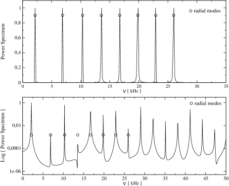
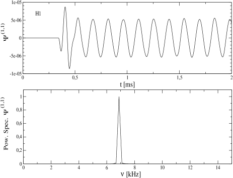
Another test of the numerical code for the radial perturbations consists in comparing the mode frequencies available in the literature, determined within a frequency domain approach, with those we obtain by applying a Fast Fourier Transformation (FFT) to the solution of our perturbative equations. In Fig. 1, we show the spectrum of the fluid velocity perturbation $\gamma^{(1,0)}$, where the radial oscillations have been excited with a selected eigenfrequency (upper panel) and with an initial Gaussian pulse (lower panel). The radial frequencies, excited during the time domain simulations, show an agreement to better than $\sim 0.2\,\%$ with the eigenfrequencies determined in Section IV.2 with a frequency domain code, and with the three known eigenfrequencies Kokkotas and Ruoff (2001).

Figure 1: Power spectrum of the radial fluid-velocity perturbation $\gamma^{(1,0)}$. The upper panel displays simultaneously the FFT of eight different time evolutions. In each evolution a single radial mode has been excited. In the lower panel, radial oscillations are excited with an initial Gaussian pulse. The circles denote the frequencies of the radial modes determined from the eigenvalue problem (see Section IV.2). Note the different horizon scales used in the panels.

In the case of the first-order axial perturbations equations, as well as in the case of the non-linear coupling, near the stellar surface we don’t have the problems exhibited by radial perturbations. Therefore, there is no need to introduce the tortoise coordinate and we can use an evenly spaced grid in $r$ ($r$-grid) for the $(0,1)$ and $(1,1)$ perturbations.

In order to build the source terms for the coupling between first-order radial and non-radial perturbations, we need to interpolate the values of radial pulsations from the $x$-grid to the $r$-grid. We find a good agreement between the evolved and interpolated radial variables when we use a $x$-grid whose resolution is twice that of the $r$-grid.

We update in time the first-order axial perturbations by using equation (50) for the axial master variable $\Psi^{(0,1)}$ and equation (51) for the axial velocity perturbation $\beta^{(0,1)}\,$. The integration of (51) is trivial: it yields a static profile for $\beta^{(0,1)}\,$. For a nonzero velocity perturbation, the master equation (50) contains a static source term. Then, the solution of (50) can be written as: $\Psi^{(0,1)}=\Psi^{(0,1)}_{h}+\Psi^{(0,1)}_{p}\,$, where $\Psi^{(0,1)}_{h}\,$ is the solution of the homogeneous equation and describes the dynamical degrees of freedom of the gravitational field, namely, it describes the gravitational wave content of the non-radial oscillations. $\Psi^{(0,1)}_{p}\,$ is a particular solution of the full equations which can be chosen to be time independent, and is related to the dragging of the inertial frames due to the stellar rotation. The homogeneous part can be obtained numerically by using a standard Leapfrog scheme (see, e.g. Press et al. (1992)). The particular solution $\Psi^{(0,1)}_{p}$ satisfies the following ordinary differential equation:

$$\Psi^{(0,1)}_{p,rr}+e^{2\Lambda}\left[4\pi r(\bar{p}-\bar{\rho})+\frac{2M}{r^{2}}\right]\Psi^{(0,1)}_{p,r} + e^{2\Lambda}\left[4\pi(\bar{p}-\bar{\rho})+\frac{6M}{r^{3}}-\frac{l(l+1)}{r^{2}}\right]\Psi^{(0,1)}_{p}$$ (66)

$$+ 16\pi re^{\Lambda}\left[\hat{\beta}_{,r}^{(0,1)}+e^{2\Lambda}\left(4\pi r\bar{p}+\frac{M}{r^{2}}\right)\hat{\beta}^{(0,1)}\right]=0\,,$$

which can be discretized in space using a second-order Finite Differences approximation and written as a tridiagonal linear system. Its solution can then be found by using a standard LU decomposition Press et al. (1992). The particular solution $\Psi^{(0,1)}_{p}$ is related to the gauge-invariant metric component $k_{0}^{(0,1)}$ through the relation (48). As it was argued in Thorne and Campolattaro (1967), it describes the frame dragging of the inertial frames due to the presence of the axial velocity perturbation:

$$-\omega(r,\theta)r^{2}\sin^{2}\theta=\mbox{g}_{t\phi}^{(0,1)}=\sum_{l,m}k_{0}^{(0,1)lm}S_{\phi}^{lm}\,,$$ (67)

where the equality $k_{0}^{(0,1)lm}=h_{0}^{(0,1)lm}$ holds in the Regge-Wheeler gauge or when the field is time independent. The metric perturbation $k_{0}^{(0,1)lm}\,$, as well as the frame dragging harmonic component $\omega^{lm}\,$, can also be determined directly from the following differential equation:

$$e^{-2\Lambda}k_{0,rr}^{(0,1)}-4\pi r(\bar{\rho}+\bar{p})k_{0,r}^{(0,1)}+\left[8\pi(\bar{\rho}+\bar{p})+\frac{4M}{r^{3}}-\frac{l(l+1)}{r^{2}}\right]k_{0}^{(0,1)}=16\pi e^{\Phi}\hat{\beta}^{(0,1)}\,,$$ (68)

which follows from (44), (48). It can be solved with the same method used for equation (66).

The linear non-radial perturbations are the combination of a gravitational wave degree of freedom and of a static solution related to the dragging of the inertial frame. They correspond, respectively, to the dynamical solution $\Psi^{(0,1)}_{h}$ and to the particular solution $\Psi^{(0,1)}_{p}$. Our tests show that $\Psi^{(0,1)}_{h}$ and $k_{0}$ have the expected second order convergence, while $\Psi^{(0,1)}_{p}$ manifests a convergence of first order. This lower convergence rate is due to the discontinuity of $\Psi^{(0,1)}_{p,rr}$ at the stellar surface.

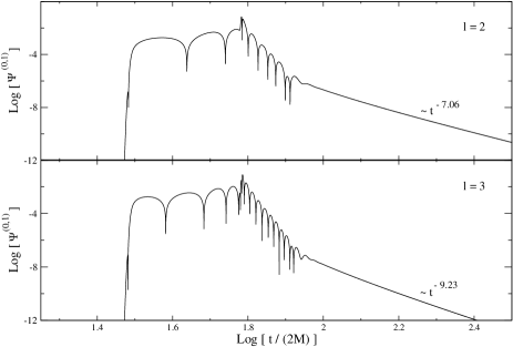
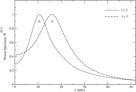
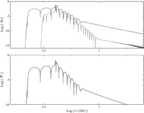
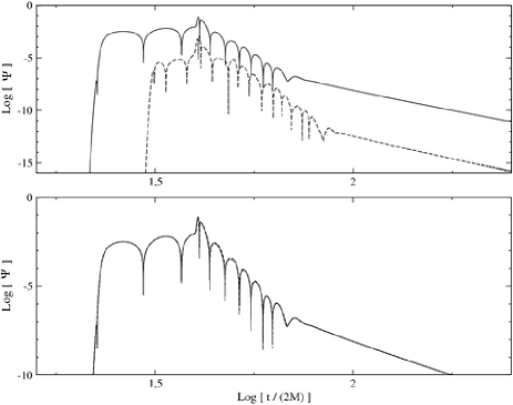
We have tested the performance of our numerical code for linear axial perturbations by comparing the results of our simulations of the scattering of an incident gravitational wave onto a compact star with results in the literature (see, e.g. Ferrari and Kokkotas (2000); Kojima and Tanimoto (2005)). For the quadrupolar case (see Fig. 2), the scattered gravitational signal exhibits the characteristic excitation of the first $w$-mode, followed by the ringing phase which is strongly damped by the emission of gravitational radiation. The behaviour of the signal at late times is known to be dominated by the gravitational-wave tails due to back-scattering of the waves by the spacetime curvature. The theoretically expected time behaviour of the tails is $\Psi^{(0,1)}\sim t^{-(2l+3)}$ (see Ching et al. (1995)). The behaviour we obtain from our simulations is shown in Fig. 2, where by using a linear regression we obtain $\Psi^{(0,1)}_{h}\sim t^{-7.1}$ for $l=2$ and $\Psi^{(0,1)}_{h}\sim t^{-9.26}$ for $l=3$. We have checked that these exponents approach the theoretical values as we increase the evolution time. The spectral properties of the solution are extracted by Fourier transforming the signal. In Fig. 3, the power spectrum curves show the excitation of the lowest order w-modes. The frequencies associated with the peaks of these curves are in excellent agreement with the frequencies computed by the frequency-domain code used in Benhar et al. (2004). Their values are: $\nu_{w}=10.501$ kHz for $l=2$ and $\nu_{w}=16.092$ kHz for $l=3$. The broad shape of the peaks is due to the short values of the w-modes damping time, $\tau=29.5$ $\mu$s for $l=2$ and $\tau=25.2$ $\mu$s for $l=3$.

Figure 2: Gravitational-wave signal determined by the scattering of a Gaussian pulse on a TOV star. The exponentially damped sinusoidal oscillations corresponds to the $l=2$ (top panel) and to the $l=3$ (bottom panel) $w$-mode ringdown. The slope of the tail is in good agreement with the theoretical prediction.

In order to test the numerical solutions of the equation (66) for the axial master function $\Psi_{p}^{(0,1)}$ (for a particular profile of the axial velocity perturbation described in subsection IV.2), we have compared the results with a different method. This alternative method consists in solving first the equation (68) for the metric perturbation $k_{0}$ and then to obtain $\Psi_{p}^{(0,1)}$ from the definition (48), which for the stationary case becomes

$$\Psi^{(0,1)}_{p}=\left(2k_{0}^{(0,1)}-rk_{0,r}^{(0,1)}\right)e^{-\left(\Phi+\Lambda\right)}\,.$$ (69)

We have found that these two different computations agree to better than $2.3\,\%$ (see Figure 6).

Figure 3: Spectrum of the first order axial perturbations due to the scattering of a Gaussian pulse on a TOV star. The peak correspond to the first $w$-mode excitation, at frequencies $\nu_{w}=10.5$ kHz ($l=2$) and $\nu_{w}=16.092$ kHz ($l=3$).

The evolution equations for the non-linear coupling perturbations, equations (62,63), have the same structure as the equations for linear axial perturbations, with the only difference that the former contain source terms. The source terms $\Sigma_{\Psi}$ and $\Sigma_{\beta}$ [their expressions are given in equations (113) and (114) respectively] are discretized by second-order centered finite difference approximations in the internal grid points and by second-order one-sided Finite Difference approximations at the origin and at the stellar surface. The computational domain for the axial master equation (62) is the entire spacetime, but the sources $\Sigma_{\Psi}$ and $\Sigma_{\beta}$ have support only in the interior spacetime (inside the star). We have tested different numerical schemes to solve the equation for the master function $\Psi^{(1,1)}$. We have found that the scheme that provides the best accuracy depends on the physical setting that we are considering. In the case we are studying the coupling between the radial pulsations and differential rotation, our calculations are more accurate when we use an upwind evolution algorithm for the interior and a leapfrog scheme for the exterior. In the case in which we study the scattering of an axial gravitational wave by a radially oscillating star, the best results are obtained when we use a Leapfrog algorithm on the whole spacetime. The reasons for this difference are the different properties of the source term $\Sigma_{\Psi}$ and the junction conditions (64) in these two different physical scenarios (see below for a description of the numerical implementation of the junction conditions). The evolution of the velocity perturbation $\hat{\beta}^{(1,1)}$ is carried out by using an up-wind scheme ($\hat{\beta}^{(0,1)}$ does not need to be evolved since it is constant in time). The solution of the axial master equation (62) and of the conservation equation (63) does not present any stability problem and the algorithm is first-order convergent. This is expected from the first order accurate numerical schemes used for the radially and differentially rotating configuration, and from the discontinuity of $\Psi^{(1,1)}_{,rr}$ at the stellar surface, due to the presence of the source terms only in the interior spacetime.

IV.2 Construction of Initial Data

In the following we describe how we prescribe initial data at the different perturbative orders: for the radial, the axial non-radial, and the coupling perturbations.

The description of the radial perturbations requires to specify initial values for $\gamma^{(1,0)}\,,$ $H^{(1,0)}\,,$ $S^{(1,0)}\,,$ and $\eta^{(1,0)}$ (although these variables are not independent since they are subject to the Hamiltonian constraint). In this paper we consider two different types of initial conditions: (i) We prescribe an initial profile for the fluid perturbations that corresponds to an eigenfunction associated with a single particular radial mode. (ii) We prescribe initially a Gaussian profile that will excite a broad range of normal radial modes.

The way in which we implement both types of initial conditions consists of setting to zero the perturbations $H^{(1,0)}\,,$ $S^{(1,0)}\,,$ $\eta^{(1,0)}$ and prescribing a non-zero initial profile for $\gamma^{(1,0)}$. For the first type of initial conditions (a single eigenmode) this implementation is equivalent to the choice of a particular time origin. Indeed, as one can find out from equations (19)-(21) and (23), we can choose consistently an oscillation normal mode with eigenfrequency $\sigma_{n}$ to have the form

$$\gamma^{(1,0)}(t,r) = \gamma_{n}^{(1,0)}(r)\cos(\sigma_{n}t)\,,$$ (70)

$$H^{(1,0)}(t,r) = H_{n}^{(1,0)}(r)\sin(\sigma_{n}t)\,,$$ (71)

$$S^{(1,0)}(t,r) = S_{n}^{(1,0)}(r)\sin(\sigma_{n}t)\,.$$ (72)

In this way we have that at $t=0$ only $\gamma^{(1,0)}$ is non-zero. For the second type of initial data (Gaussian profile) our choice of implementation is not the most general one, it just represents a particular linear combination of eigenmodes.

To construct the first type of initial data, we can set up the eigenvalue problem for the radial velocity perturbation $\gamma^{(1,0)}\,$, from the wave-type equation that can be derived from equations (19) and (20):

$$\left(P(r)y^{(1,0)}_{,r}\right)_{,r}+Q(r)y^{(1,0)}-W(r)y_{,tt}^{(1,0)}=0\,,$$ (73)

where $y^{(1,0)}=r^{2}e^{-\Lambda}\gamma^{(1,0)}=r^{2}e^{-\Phi}\xi^{r}_{,t}$, and $\xi^{r}$ is the Lagrangian displacement of the radial oscillations. The functions $W,P,Q$ are constructed from quantities associated with the TOV background:

$$r^{2}W=(\bar{\rho}+\bar{p})e^{3\Lambda+\Phi}\,,$$ (74)

$$r^{2}P=(\bar{\rho}+\bar{p})\bar{c}_{s}^{2}e^{\Lambda+3\Phi}\,,$$ (75)

$$r^{2}Q=(\bar{\rho}+\bar{p})\left[\Phi_{,r}\left(\Phi_{,r}-\frac{4}{r}\right)-8\pi\bar{p}e^{2\Lambda}\right]e^{\Lambda+3\Phi}\,.$$ (76)

By making the substitutions $y^{(1,0)}=y_{0}(r)e^{i\omega t}$ and $z^{(1,0)}=Py_{,r}^{(1,0)}$ in equation (73) we obtain the following pair of first-order equations

$$y_{,r}^{(1,0)} = P^{-1}z^{(1,0)}\,,$$ (77)

$$z_{,r}^{(1,0)} = -(\omega^{2}W+Q)y^{(1,0)}\,.$$ (78)

To complete the eigenvalue problem we need to prescribe boundary conditions at the origin and at the surface location. At the origin, from the regularity condition (28), we must have the following behaviour

$$y^{(1,0)}(r)=y_{0}r^{3}\,,\quad z^{(1,0)}(r)=z_{0}^{(1,0)}\,,$$ (79)

which combined with equation (77) yields the following boundary condition:

$$y_{0}=\textstyle{\frac{1}{3}}P^{-1}z_{0}\,.$$ (80)

Figure 4: Eigenfunctions for the radial velocity perturbation $\gamma^{(1,0)}$ corresponding to the fundamental mode and the first seven overtones.

Table 2: Eigenfrequencies (in kHz) of the first eight normal modes of the radial perturbations. The second column corresponds to the results from calculation in the frequency domain (the solution of the Sturm-Liouville problem). The third column corresponds to the results from a time-domain calculation, after applying a FFT to the resulting time series. The fourth column shows the first three normal modes computed by Kokkotas and Ruoff Kokkotas and Ruoff (2001).

Mode	Frequency domain	Time domain	From Kokkotas and Ruoff (2001)
F	2.138	2.145	2.141
H1	6.862	6.867	6.871
H2	10.302	10.299	10.319
H3	13.545	13.590
H4	16.706	16.737
H5	19.823	19.813
H6	22.914	22.889
H7	25.986	25.964

The boundary condition at the surface comes from the vanishing of the Lagrangian pressure perturbation there. The resulting condition reads [see equation (24)]:

$$(\bar{\rho}+\bar{p})\bar{c}^{2}_{s}y^{(1,0)}_{,r}|_{r=R}=0\,.$$ (81)

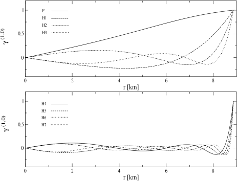
The eigenvalue problem can be solved numerically by using a standard relaxation method (for details see Press et al. (1992)). As discussed above, in order to obtain accurate evolutions of radial perturbations it is convenient to introduce the fluid tortoise coordinate (65) which provides the necessary resolution close to the stellar surface. The equations that one obtains for the eigenvalue problem in terms of the fluid tortoise coordinate have been given in Appendix C. The eigenfrequencies and the associated eigenfunctions for the fundamental mode and the first seven overtones of the radial velocity $\gamma^{(1,0)}$ are shown in table 2 and in Fig. 4 respectively. They have been normalized with respect to the absolute value of their maximum. Our computations of the eigenfrequencies and the associated eigenfunctions have second-order convergence.

In the case of the first-order axial non-radial perturbations, we need to prescribe initial data for $\Psi^{(0,1)}$ at its time derivative at an initial time $t=t_{o}\,,$ say $(\Psi^{(0,1)}_{o},\partial_{t}\Psi^{(0,1)}_{o})\,$, and a certain profile for $\hat{\beta}^{(0,1)}\,$, or equivalently for $\beta^{(0,1)}$ (this quantity remains contant along the evolution). Specifying this profile is equivalent to prescribe a certain differential rotation law for the star Thorne and Campolattaro (1967); Gundlach and Martín-García (2000). As we have discussed before, this law has an impact on the evolution of $\Psi^{(1,0)}\,$, and it induces a dragging of inertial frames. In this work we consider two types of initial data for the first-order axial perturbations: (i) we prescribe a certain rotation law $\beta^{(0,1)}\,$, and then we obtain a profile for $\Psi^{(0,1)}_{o}$ from the integration of equation (66) which corresponds to the particular solution $\Psi^{(0,1)}_{p}$. For the homogeneous part of $\Psi^{(1,1)}$, the dynamical one, we specify zero data: $(\Psi^{(0,1)}_{h,o},\partial_{t}\Psi^{(0,1)}_{h,o})=(0,0)\,$. (ii) We set the star rotation to zero: $\beta^{(0,1)}=0$. Then, we just set the particular solution $\Psi^{(0,1)}_{p}$ equal to zero and prescribe arbitrary profiles for the homogeneous part: $(\Psi^{(0,1)}_{h,o},\partial_{t}\Psi^{(0,1)}_{h,o})\,.$

In order to discuss the first type of initial data it is important to mention that presently there is no sufficient knowledge on the laws of differential rotation for neutron stars. For nearly born neutron stars, one may obtain a description of the rotation law from the numerical simulations of core collapse (see, e.g. Zwerger and Mueller (1997); Dimmelmeier et al. (2002a, b)). In the Newtonian approach, a set of rotation laws has been introduced motivated by mathematical simplicity and the aim of satisfying Rayleigh’s stability criterion for rotating inviscid fluids:

$$d(\varrho^{2}\Omega)/d\varrho>0\,,$$ (82)

where $\varrho=r\sin\theta$ is the cylindrical radial coordinate and $\Omega=\Omega(r,\theta)$ is the angular velocity measured by an observer at infinity and describes the stellar differential rotation. Among this family of Newtonian rotation laws there is one, the j-constant law, that has been incorporated into a General Relativistic approach Komatsu et al. (1989a, b) by taking into consideration the dragging of the inertial frames. In this work, we introduce a rotation law by prescribing the velocity perturbation $\beta^{(0,1)}_{lm}$ from an expansion in (vector) spherical harmonics of the velocity perturbation of a slowly differentially rotating star. In the slow rotation approximation, the fluid velocity perturbation is given by

$$u_{\mu}^{(0,1)}=\left(0,u_{a}^{(0,1)}\right)=e^{-\Phi}\left(0,0,0,r^{2}\sin^{2}\theta\,\left(\Omega-\omega\right)\right)\,,$$ (83)

where $\Omega=\Omega(r,\theta)$ is the angular velocity measured by an observer at infinity and describes the stellar differential rotation, while the function $\omega=\omega(r,\theta)$ describes the dragging of inertial frames associated with the stellar rotation. In the case of barotropic rotating stars, the integrability condition of the hydrostatic equilibrium equation requires that the specific angular momentum measured by the proper time of the matter is a function of $\Omega$ only Komatsu et al. (1989a), that is, $u^{t}u_{\phi}=j(\Omega)$. In the slow rotation approximation this condition leads to the following expression:

$$j^{(0,1)}(\Omega)=u^{t}u_{\phi}^{(0,1)}=e^{-2\Phi}r^{2}\sin^{2}\theta\,\left(\Omega-\omega\right)\,,$$ (84)

which is a linear approximation in $\Omega$. The choice of the functional form of $j(\Omega)$, and hence of $j^{(0,1)}(\Omega)$, must satisfy the Rayleigh’s stability criterion against axisymmetric disturbances for inviscid fluid:

$$\frac{d\,\tilde{\jmath}}{d\Omega}<0\,,$$ (85)

where $\tilde{\jmath}$ is the specific angular momentum

$$\tilde{\jmath}=(\bar{\rho}+\bar{p})\frac{u_{\phi}}{\bar{\rho}_{0}}$$ (86)

and $\bar{\rho}_{0}$ is the rest mass density. The specific angular momentum $\tilde{\jmath}$ is locally conserved during the axisymmetric collapse of a perfect fluid Stergioulas et al. (2004). A common choice for $j(\Omega)$ that satisfies these conditions Komatsu et al. (1989a, b) is the following:

$$j^{(0,1)}(\Omega)=A^{2}\left(\Omega_{c}-\Omega\right)\,,$$ (87)

where $\Omega_{c}$ is the angular velocity at the rotation axis and $A$ is a constant that describes the amount of differential rotation. We can now find the rotation law from equations (84) and (87). The result is:

$$\Omega(r,\theta)=\frac{A^{2}\Omega_{c}+e^{-2\Phi}r^{2}\sin^{2}\theta\,\omega(r,\theta)}{A^{2}+e^{-2\Phi}r^{2}\sin^{2}\theta}\,.$$ (88)

In the Newtonian limit this equation reduces to the $j$-constant rotation law used in Newtonian analysis Hachisu (1986):

$$\Omega(r,\theta)=\frac{A^{2}\Omega_{c}}{A^{2}+r^{2}\sin^{2}\theta}\,.$$ (89)

A uniform rotating configuration with $\Omega=\Omega_{c}$ is attained for high values of $A$ ($A\rightarrow\infty$). On the other hand, for small values of $A$, the law (88) describes, in the Newtonian limit, a configuration with constant angular momentum.

The only non-vanishing vector spherical harmonic components of $u_{a}^{(0,1)}$ are given by the expansion

$$u_{\phi}^{(0,1)}=\sum_{l,m}\beta_{lm}^{(0,1)}S_{\phi}^{lm}\,,$$ (90)

where $\beta^{(0,1)}_{lm}$ are the velocity perturbations (which depend on the coordinate $r$) that were introduced in equation (42) [we have now restored the spherical harmonic indices $(l,m)$]. The different $\beta_{lm}^{(0,1)}$ are obtained by using the properties of the inner product among the different elements of the basis of axial vector spherical harmonics. Their expression is

$$\beta_{lm}^{(0,1)}=\frac{1}{\sqrt{l(l+1)}}\,\int_{S^{2}}\sin\theta d\theta d\phi\,u_{a}^{(0,1)}S_{b}^{lm}\gamma^{ab}\,,$$ (91)

where $\gamma^{ab}$ is the contravariant metric on $S^{2}$.

In order to determine the initial profile for the axial velocity perturbations we just have to introduce the rotation law (88) into the form of the velocity perturbations (83). We obtain

$$u_{\phi}^{(0,1)}=\frac{e^{-\Phi}A^{2}}{A^{2}+e^{-2\Phi}r^{2}\sin^{2}\theta}\left(r^{2}\sin^{2}\theta\,\Omega_{c}+\sum_{lm}k_{0}^{lm}S_{\phi}^{lm}\right)\,,$$ (92)

where we have used equation (67), which relates the metric perturbations with the frame dragging function $\omega\,.$ It is important to notice that the first term in (92) corresponds to the the Newtonian j-rotation law (up to the factor $e^{-\Phi}$), to which we will refer as the nearly Newtonian j-rotation law. The other terms account for the dragging of the inertial frames. To obtain the velocity perturbations $\beta^{(0,1)}_{lm}$ from (91) we just need to introduce there expression (92). In doing this, we can easily determine the expression for the nearly Newtonian term, but we need to pay special attention to the relativistic corrections. The difficulty arises from the expansion in axial vector harmonics in (92) containing the unknowns, $k_{0}^{lm}$, of the differential equation (68). Due to the form of (92), the inner product in equation (91) will contain products of harmonics with different harmonic indices. In order to decouple these terms in the relativistic corrections we assume that the dominant contributions are provided by the metric perturbations $k_{0}^{lm}$ that have the same harmonic indices as in the nearly Newtonian rotation law. For the nearly Newtonian part, we have found solutions only for $A>e^{-\Phi(R_{s})}R_{s}$. From this relation and from the values assumed by the metric function $\Phi$ in the stellar model considered in this work (see subsection III.1) we can give the following estimation for the allowed values of $A$:

$$\frac{1}{2}<\frac{A^{2}}{A^{2}+e^{-2\Phi}r^{2}\sin^{2}\theta}\leq 1\,.$$ (93)

Then, using these inequalities, the approximation that we obtain for the relativistic terms of equation (92) is given by:

$$u_{\phi}^{(0,1)}=\frac{A^{2}r^{2}\sin^{2}\theta\,e^{-\Phi}\,{}}{A^{2}+e^{-2\Phi}r^{2}\sin^{2}\theta}\,\Omega_{c}+\alpha_{0}e^{-\Phi}\sum_{lm}k_{0}^{lm}S_{\phi}^{lm}\,,$$ (94)

where here $\alpha_{0}$ is a constant such that $\alpha_{0}\in(0.5,1]$. The coefficients of the expansion of this equation in axial vector harmonics have the following form

$$u_{\phi,l0}^{(0,1)}=\left\{\begin{array}[]{ll}\alpha_{0}e^{-\Phi}k_{0}^{l0}S_{\phi}^{l0}&\quad\textrm{for}~{}l~{}\textrm{even}\,,\\ \\ \beta^{(0,1)}_{l0}S_{\phi}^{l0}&\quad\textrm{for}~{}l~{}\textrm{odd}\,,\end{array}\right.$$

where the coefficients of the components with odd $l$ are given by the following expression:

$$\beta^{(0,1)}_{l0}=\frac{e^{\Phi}\Omega_{c}}{\sqrt{l(l+1)}}f_{l0}\left(x,A\right)+\alpha_{0}e^{-\Phi}\,k_{0}^{l0}\,,$$ (95)

where $x=re^{-\Phi}$ (not to be confused with the fluid tortoise coordinate). The functions $f_{l0}(x,A)$ for $l=1$ and $l=3$ are given by the following expressions

$$f^{(0,1)}_{10} = -4.342A^{2}\left[1-\frac{A^{2}}{x\sqrt{A^{2}+x^{2}}}\ln\left(\frac{\sqrt{\sqrt{A^{2}+x^{2}}+x}}{\sqrt{\sqrt{A^{2}+x^{2}}-x}}\right)\right]\,,$$ (96)

$$f^{(0,1)}_{30} = -2.708A^{2}\left[1+7.5\frac{A^{2}}{x^{2}}-\frac{6A^{2}}{x\sqrt{A^{2}+x^{2}}}\left(1+\frac{5}{4}\frac{A^{2}}{x^{2}}\right)\ln\left(\frac{\sqrt{\sqrt{A^{2}+x^{2}}+x}}{\sqrt{\sqrt{A^{2}+x^{2}}-x}}\right)\right]\,.$$ (97)

which have been derived by imposing the condition $A>R_{s}e^{-\Phi(R_{s})}$.

Figure 5: Profiles of the $l=3$ component of the axial velocity perturbation $\beta^{(0,1)}_{30}$ determined for a $j$-rotation law with $A=10$ km and a rotation period at the axis of $T=10$ ms. The solid line corresponds to the axial velocity associated with the nearly Newtonian $j$-law, while the dotted and dashed lines correspond to the velocity perturbations in (95) with $\alpha=0.5$ and $\alpha=1$ respectively.

In the limit of $A\rightarrow\infty$, the functions $f_{l0}$ behave as expected, that is, the nearly Newtonian part becomes:

$$\lim_{A\rightarrow\infty}\frac{e^{\Phi}\Omega_{c}}{\sqrt{l(l+1)}}f_{l0}S_{\phi}^{l0}=\left\{\begin{array}[]{ll}e^{-\Phi}\Omega_{c}r^{2}\sin^{2}\theta&\quad\textrm{for}~{}l=1\,,\\ \\ 0&\quad\textrm{for}~{}l\geq 3\,,\end{array}\right.$$

which corresponds to a uniformly rotating configuration, where $\Omega=\Omega_{c}$ is the angular velocity as measured at infinity. Since in this work we are mainly interested in the impact of the non-linear coupling of the stellar oscillations in the gravitational wave emission, we will consider only the case $l=3$, as the dipolar term $l=1$ does not produce gravitational waves.

In Fig. 5 we plot the profiles for the axial velocity perturbation $\beta_{30}^{(0,1)}$. It shows that the two solutions corresponding to the extreme values of the constant $\alpha_{0}$ disagree in an amount below $10\,\%$. In the following simulations we will use for simplicity only the nearly Newtonian term by obtaining results which are correct to better than $10\,\%$.

Figure 6: The stationary axial master function $\Psi^{(0,1)}_{p}$ relative to a nearly Newtonian $j$-rotation law with $A=15$ km and a period $T=10$ ms at the rotation axis (top panel). The solution of the equation (66) is showed with the solid line while the dashed line denotes the solution found indirectly by first solving Eq. (68) for the variable $k_{0}^{(0,1)}$ and then using the definition (69). The frame dragging function $\omega_{30}$ determined by the initial value (95) is displayed in the bottom panel.

With regard to second choice of initial conditions for the axial non-radial perturbations, namely $\beta^{(0,1)}=0\,$, it is going to be used in this paper to investigate how the second-order metric perturbations corresponding to the coupling terms can be affected by the radial pulsations of the star. Actually, it is well known that the axial components of the gravitational-wave signal emitted by a non-rotating compact star can only contain the imprint of the spacetime $w$-modes. The question we can ask is then how this particular signal looks like when it couples with the radial pulsations of the star. What we do in practice is to generate $w$-modes at first-order and to study the corresponding signal at second-order (in the sector of the coupling of radial and non-radial modes) by looking at its dependence on the radial pulsations of the star. The $w$-mode oscillation is excited by the standard procedure of scattering a (narrow) Gaussian pulse of gravitational waves on the star.

For the non-linear coupling perturbations we have to prescribe initial data for $\Psi^{(1,1)}$, $\Psi^{(1,1)}_{,t}$ and $\beta^{(1,1)}$ at an initial time $t=t_{o}$. Since we are mostly interested in the non-linear effects generated from the coupling between linear perturbations and not in the evolution per se of second-order perturbations, we set these quantities initially to zero.

To sum up, combining the different types of initial data for the first-order perturbations we can study the following two different scenarios: (i) the scattering of a gravitational wave by a radially oscillating star. (ii) A radially pulsating star with with differential rotation.

IV.3 Boundary conditions

The behaviour at the stellar center of the radial, axial non-radial, and non-linear coupling perturbations is given in equations (25)-(28) and (55). In order to deal numerically with the centrifugal term of the potential of the axial master equation, $l(l+1)r^{-2}$, we use a numerical grid where the first grid-point, $r_{1}\,$, does not coincide with the center $r=0$ but instead is located at $r_{1}=\Delta r\,$, being $\Delta r$ the grid spacing. Then, we impose at $r_{1}$ the regularity conditions (25)-(28) and (55). For instance, in the case of the variable $\Psi^{(0,1)}$, which behaves as $\Psi_{0}(t)r^{l+1}$ [equation (55)], we assume that this behaviour is in a good approximation also valid at the grid points $r_{1}$ and $r_{2}$, and then we determine the value of $\Psi^{(0,1)}$ at $r_{1}$ from the following relation:

$$\Psi^{(0,1)}(r_{1})=\Psi^{(0,1)}(r_{2})\left(\frac{r_{1}}{r_{2}}\right)^{l+1}\,.$$ (98)

Let us consider now the boundary conditions at the stellar surface, where the pressure vanishes. In this way, the unperturbed stellar surface is $\bar{\Sigma}=\{x~{}|~{}r(x)=R_{s}\}$ where $R_{s}$ is the stellar radius of the TOV model, where the background pressure $\bar{p}$ vanishes. Due to the radial pulsations, the surface of the perturbed star does not coincide with the static surface, but is given by $\Sigma\equiv\{x+\lambda\xi^{(1,0)}~{}|~{}x\in\bar{\Sigma}\}\,$, where $\xi^{(1,0)}$ is the Lagrangian displacement vector of a fluid element. The axial non-radial modes only induce rotation of the star and hence, they do not change the shape of the stellar surface. Therefore, at first order we have to impose the vanishing of the total pressure on the perturbed surface $\Sigma$ for the radial perturbations, which is equivalent to the relation (24), and the continuity conditions on the static surface for the axial non-radial perturbations.

The radial perturbations are evolved using the x-grid (the one determined by the fluid tortoise coordinate), then we interpolate the solution to the r-grid (the one determined by the area radial coordinate). In terms of the fluid tortoise coordinate $x$, the surface condition (24) is given in equation (128) of Appendix C, with $R_{x}$ being the value of the fluid tortoise coordinate corresponding to the static stellar radius $R_{s}$. This condition will be certainly satisfied by finite values for $\gamma^{(1,0)}$ and $\gamma^{(1,0)}_{,x}$, since pressure, density and speed of sound go to zero at the surface for a polytropic equation of state. We then determine, at every time step, the finite value of $\gamma^{(1,0)}$ on the surface by using a second-order polynomial extrapolation. The surface boundary conditions for the other three radial variables are then directly determined from the perturbative equations.

The solution of the axial master equation (50) is decomposed into two pieces: an homogeneous part $\Psi_{h}^{(0,1)}$ that satisfies the homogeneous equation, and a static particular solution $\Psi_{p}^{(0,1)}$ that satisfies the equation (66). These equations are solved numerically on the whole spatial grid without imposing junction conditions. In this way, the continuity of $\Psi_{h}^{(0,1)}$ and $\Psi_{p}^{(0,1)}$ and its first spatial derivatives, required by the junction conditions described in Section III.3, follows automatically.

The junction conditions for the non-linear perturbations require some approximations (see Sperhake (2001); Sperhake et al. (2001) for a treatment of the junction conditions in a similar non-linear context). In an Eulerian gauge the perturbed surface will not coincide in general with the surface of the background equilibrium configuration. As a consequence, some perturbative quantities may take unphysical values near the surface during the expansions and contraction phases of the star. For instance, while the background enthalpy and density go to zero as we approach the static stellar surface, the associate radial perturbations have an oscillatory character with amplitudes that, near the surface, are bigger than the background values. Therefore, in a contraction phase, when the Eulerian radial perturbations of enthalpy and density are negative, the total mass-energy $\bar{\rho}+\delta\rho^{(1,0)}$ may take negative values. Furthermore, the low densities which are present at the outermost layers of the star may also produce some numerical errors in the simulations Harada et al. (2003). These problems can be avoided if we do not impose the matching conditions for the non-linear perturbations at the static stellar surface, as we do for the linear perturbations, but at a hypersurface that during the evolution remains always slightly inside the unperturbed star Sperhake (2001); Harada et al. (2003). In practice this procedure is implemented as follows: (i) we estimate the amplitude of the surface movement due to radial pulsations. (ii) We compute the linear (radial and non-radial) perturbations up to the static surface $R_{s}$. (iii) We impose the junction conditions for the non-linear perturbations on a hypersurface that is always inside (even during the contraction phase) the unperturbed star. (iv) We estimate the effects on the gravitational signal. In this sense, it is important to mention that in doing this approximation we are removing the outer layers of the star, where the density is very low, which in practice means that we are neglecting less than one percent of the stellar mass, which does not produce significative changes in the waveforms and spectra of the gravitational signal. Moreover, by using an appropriate choice of initial conditions, the movement of the perturbed surface due to radial pulsations can be very small $\sim 10^{-3}R_{s}$. Therefore, this approximative procedure leads to neglect only one or two grid points near the stellar surface. However, on the negative side, since the source term for the axial master equation (62) takes its maximum amplitude at the stellar surface, this removal of one or two grid points induces an error of about $5\,\%$ in the gravitational wave signal.

The procedure we have just described allows us to simplify the junction condition (64) for the two initial configurations that we consider in this paper. In the case of the scattering of an axial gravitational wave by a radially pulsating star, the velocity perturbations $\hat{\beta}^{(0,1)}$ and $\hat{\beta}^{(1,1)}$ are set to zero. Therefore, by using the continuity of the first order perturbations, the junction condition (64) reduces to the continuity of $\Psi^{(1,1)}_{,r}$. We then evolve the axial master equation (62) for $\Psi^{(1,1)}$ on the whole numerical grid, with the source terms only present in the interior of the star. In this way the junction conditions on the matching surface are automatically satisfied. For the second situation that we study, the non-linear coupling in a radially pulsating and differentially rotating star, we can only use the continuity of the linear perturbations to reduce (64) to the following expression:

$$e^{-\Lambda}\Psi^{(1,1)}_{,r}+16\pi r\hat{\beta}^{(1,1)}\,.$$ (99)

In this case, the numerical procedure to solve the axial master equation (62) goes as follows: (i) In the interior spacetime we implement an up-wind scheme. (ii) At the matching hypersurface, the junction conditions provide the values of the axial function $\Psi^{(1,1)}$ and its time and spatial derivatives. (iii) Finally, the values obtained at the matching hypersurface are used to evolve the axial master function $\Psi^{(1,1)}$ in the exterior (the $(1,1)$ Regge-Wheeler equation) by using a Leapfrog scheme.

Figure 7: Waveforms (in logarithmic scale) from the scattering of an $l=2$ axial gravitational wave from a star oscillating radially in the fundamental mode (see Table 2). The top panel presents the first-order axial non-radial master function $\Psi^{(0,1)}$ (solid line) and the second-order coupling function $\Psi^{(1,1)}$ (dashed line). The bottom panel exhibits the waveform $\Psi^{(0,1)}$ (solid line) together with the total signal $\Psi^{(0,1)}+\Psi^{(1,1)}$ (dashed line).

V Results

The following section is devoted to discuss the results of time-domain numerical simulations describing the non-linear coupling of radial and axial non-radial oscillations of a static star in two different physical settings: (i) The scattering of a gravitational wave by a radially pulsating star (subsection V.1). (ii) A differentially rotating and radially oscillating star (subsection V.2).

V.1 Effects of radial pulsations on the scattering of a gravitational wave

The aim of these simulations is to investigate the possible signature of the radial oscillations of the star in scattered gravitational waves. The initial first order axial perturbation correspond to an $l=2$ mode with vanishing velocity perturbation $\beta^{(0,1)}$. The profile of the axial master function $\Psi^{(0,1)}$ is a Gaussian pulse

$$\Psi^{(0,1)}(t_{o},r)=A^{(0,1)}e^{-q(r-r_{0})^{2}}\,,$$ (100)

centered at $r_{0}=20$ km with amplitude $A^{(0,1)}=0.1$ and width parameter $q=1.25$. The star oscillates in one of the radial eigenmodes corresponding to the frequencies of Table 2.

In Figs. 7 and 8, we present the $l=2$ waveforms associated with the first-order axial non-radial master function $\Psi^{(0,1)}$ and the master function $\Psi^{(1,1)}$ describing the coupling. We find that the correction to the signal coming from the coupling is less than $2\,\%$ when the radial pulsations are excited by the F-modes, and less than $0.1\,\%$ for higher overtones. These corrections do not modify the properties of the waveforms and spectra associated with the first-order perturbations. We find similar results for higher overtones and their combinations. In summary, in this particular scenario we have not found any significant amplification of the gravitational wave signal due to the coupling of the radial and axial non-radial first-order perturbations.

Figure 8: Waveforms (in logarithmic scale) from the scattering of an $l=2$ axial gravitational wave from a star oscillating radially in the first overtone H1 (see Table 2). The top panel presents he first-order axial non-radial master function $\Psi^{(0,1)}$ (solid line) and the second-order coupling function $\Psi^{(1,1)}$ (dashed line). The bottom panel exhibits the waveform $\Psi^{(0,1)}$ (solid line) together with the total signal $\Psi^{(0,1)}+\Psi^{(1,1)}$ (dashed line).

V.2 Coupling between radial pulsations and differential rotation

The aim of the simulations we present in this subsection is to investigate the effect of the coupling of radial oscillations with differential rotation, as described by axial non-radial first-order perturbations, in the gravitational wave signal. The axial rotation of the fluid is described with a good approximation by the nearly Newtonian $j$-constant rotation law described in the subsection IV.2. All the simulations in this subsection have a first-order rate of convergence and are long term stable.

V.2.1 Single radial mode oscillation

We start with simulations in which we consider single mode excitation of the radial oscillations, in particular the first overtone H1. The initial velocity perturbation $\gamma^{(1,0)}$ is taken to be [see equation (70)]

$$\gamma^{(1,0)}=G^{(1,0)}\gamma^{(1,0)}_{n}\,,$$ (101)

with $G^{(1,0)}=0.001$. For this amplitude we can be sure that the region of the spacetime that the motion of the surface covers is confined to a narrow slice around the static equilibrium configuration. Therefore, the issues related to negative values of the mass-energy density in an Eulerian description can be solved approximatively as we explained above.

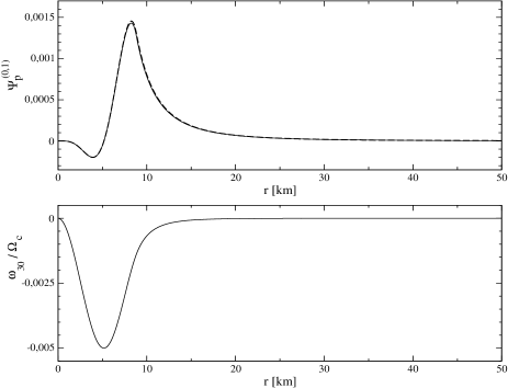
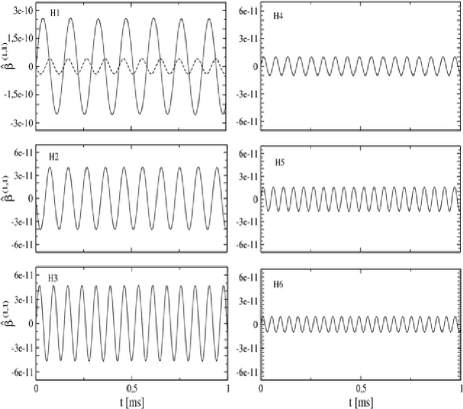
The values of the differential rotation parameter $A$ and the angular velocity at the rotation axis in these simulations are $A=15$ km and $\Omega_{c}=2.09\times 10^{-3}$ km^-1. This latter (corresponding tp a period of $10$ ms) is small compared with the mass shedding limit value $\Omega_{K}$: $\Omega_{c}/\Omega_{K}=6.45\times 10^{-2}$. The profile of the axial velocity perturbation $\beta^{(0,1)}$ for $l=3$ is given in equation (97) and depicted in Fig. 5. For this initial configuration of the differential rotation, the coupling non-linear perturbations are dominated by the harmonic $l=3\,$.

Figure 9: Coupling between radial mode oscillations (overtone H1) and differential rotation (with rotation period $T=10$ ms). Waveform $\Psi^{(1,1)}$ for $l=3$ multipole (top panel). A (transient) excitation of the first $l=3$ $w$-mode at early times is present, followed then by a periodic oscillation driven by the radial mode. The Fourier spectrum of the periodic oscillation (bottom panel) is dominated by the frequency $\nu_{\rm H1}\simeq 6.8$ kHz corresponding to the H1 radial pulsation.

In Fig. 9 we show the $l=3$ waveform (top panel) extracted at $100$ km apart from the stellar center: after an initial transient phase dominated by $w$-mode ringing (see below), the $\Psi^{(1,1)}$ waveform exhibits a monocromatic oscillation at the frequency of the H1 mode; i.e., $\nu_{\rm H_{1}}\approx 6.8$ kHz, as confirmed by the Fourier spectrum of the signal (bottom panel). The presence of the $w$-mode in the initial phase of the waveform is related to the choice of initial data that we have done for simplicity; i.e., $\Psi^{(1,1)}=\Psi^{(1,1)}_{,t}=\beta^{(1,1)}=0$. This is, in general, non consistent, because these three quantities are not independent; indeed, a correct set up of the initial data for $\Psi^{(1,1)}$ would require the solution of the “coupling” axial constraints (not reported here) in a way similar to what is usually done for the first-order polar and axial perturbations (see for example Ref. Nagar and Rezzolla (2005)). If this is not done, the system requires to relax to the “correct” solution through the release of a GWs burst of $w$-modes. However, since our interest is focused here on the stationary phase driven by the radial oscillations of the star, we decided to avoid the complications related to correctly capture the initial transient.

V.2.2 Amplification effects

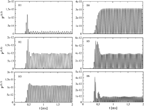
In this section we extend the previous analysis to simulations where the radial pulsations are excited using combinations of the fundamental mode and higher overtones. In general, the waveforms and spectra present the same features as the H1 case described above. However, an interesting amplification is observed in simulations where the radial oscillations contain a frequency close to the one of the axial $w$-mode. In Fig. 10, we show the axial master function $\Psi^{(1,1)}$ for six runs using different radial overtones. It is clear there that $\Psi^{(1,1)}$ increases in amplitude as we increase the order of the radial normal mode from the first to the fourth overtone, while it decreases as we go to the fifth and sixth overtones. The amplitude of $\Psi^{(1,1)}$ for the H4 case is about sixteen times that of $\Psi^{(1,1)}$ for the H1 case. For this stellar model, the $l=3$ spacetime mode has frequency $16.092$ kHz which is between the frequencies of the third and fourth radial overtones, $13.545$ kHz and $16.706$ kHz respectively. Moreover, this effect takes place despite the energy and the maximum displacement of the surface of the radial modes decrease proportionally to the order of the radial modes (see Table 3). The interpretation of this amplification as a sort of resonance effect is supported by the structure of the axial master equation (62) and its analogy with a forced oscillator. The amplification arises when one of the natural frequencies, determined by the form of the axial potential $V$ [see equations (54, 62)], is sufficiently close to the frequency (or frequencies) associated with the external force. In the case when the non-radial perturbations are static and just describe differential rotation, the frequencies corresponding to the external force are determined by the structure of the radial oscillations. This picture is confirmed by the fact that this amplification effect disappears when the axial potential is arbitrarily removed. In addition, the fluid velocity perturbation $\hat{\beta}^{(1,1)}$, which satisfies a completely different equation (63), does not show any such amplification and instead decreases proportionally with the order of the radial mode (see Fig. 11).

Figure 10: Comparison of six $\Psi^{(1,1)}$ waveforms for the $l=3$ multipole. The differential rotation law is the same as the one used in Fig. 9. The radial pulsations considered correspond to single mode oscillation from H1 to H6 overtone. These plots show that a resonance effect take place in $\Psi^{(1,1)}$. See text for a discussion.

Table 3: Quantities associated with radial normal modes and their coupling to the first-order axial differential rotation: Energy, $E^{(1,0)}_{n}$, and maximum stellar surface displacement $\xi^{(1,0)}_{\rm sf}$ of the radial eigenmodes [From initial conditions (101) with $G^{(1,0)}=0.001$]; power, $\dot{E}^{(1,1)}_{30}$, emitted in gravitational waves to infinity from the coupling between the radial eigenmode and the axial differential rotation; estimated values of the damping times, $\tau^{(1,1)}_{30}\,;$ and number of oscillation periods, $N_{\rm osc}\,,$ that takes for the non-linear oscillations to radiate the total energy initially contained in the radial modes.

Normal Mode:	F	H1	H2	H3	H4	H5	H6
$E^{(1,0)}_{n}~{}[10^{-8}$ km]	$35.9$	$4.2$	$1.37$	$0.62$	$0.34$	$0.21$	$0.14$
$\xi^{(1,0)}_{\rm sf}$ [m]	$12.65$	$4.02$	$2.66$	$2.02$	$1.64$	$1.38$	$1.19$
$<\dot{E}^{(1,1)}_{30}>~{}[10^{-13}]$	$1.85\times 10^{-6}$	$6.83\times 10^{-2}$	$4.85$	$56.03$	$157.01$	$19.08$	$4.45$
$\tau^{(1,1)}_{30}$ [ms]	$6.49\times 10^{9}$	$20.49\times 10^{3}$	$94.15$	$3.69$	$0.72$	$3.67$	$10.51$
$N_{\rm osc}$	$1.39\times 10^{10}$	$1.408\times 10^{5}$	$971.58$	$49.99$	$12.07$	$72.78$	$240.77$

Figure 11: Time evolutions (the same runs as in Fig. 9) of the second-order fluid velocity perturbation $\hat{\beta}^{(1,1)}\,$. The perturbation $\hat{\beta}^{(1,1)}$ has been averaged over the star at each time step and plotted here. The dashed line in the left top panel (H1) reports the perturbation for the H2 eigenmode and is superposed for comparison.

In agreement with these results, the power emitted in gravitational waves to infinity exhibits the same amplification too (see Fig. 12). There are obviously two different contributions to the power, one due to the $w$-mode excitation related to the initial data choice and the second related to the periodic emission driven by the stellar radial pulsations. The relative strength of these two contributions to the power changes as we change the radial eigenmode. The periodic emission increases for the first eigenmodes and reaches its maximum for the H4 overtone; it decreases then for H5 and H6.

Figure 12: Emitted power in gravitational waves $P^{(1,1)}=\dot{E}_{30}^{(1,1)}$ for the six runs of Fig. 10.

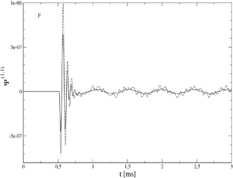
Let us now look at the coupling between differential rotation and radial pulsations in the fundamental mode F. The $\Psi^{(1,1)}$ waveform is reported in Fig. 13. After the initial $w$-mode transient, the signal is dominated by a periodic pulsation at the radial F-mode frequency. We notice that the amplitude of the oscillation is smaller than in the previous cases due probably to the fact that the radial F-mode frequency is not enough close to the first $w$-mode frequency. The periodic part of the signal exhibits high frequency oscillations associated with the low density region near the stellar surface: in Fig. 13 we depict (with a dashed line) the waveform obtained when the junction conditions have been imposed at a radial coordinate $r=8.64$ km, (which is equivalent to neglect $0.3\,\%$ of the stellar mass) and with a solid line the case when the matching surface stands at $r=7.75$ km (corresponding to neglecting a $6.3\,\%$ of the total mass). In the later case the numerical noise is reduced and the waveform looks closer to the expected form.

Our perturbative approach does not include backreaction (see, e.g. Balbinski et al. (1985); Yoshida and Eriguchi (1995)); in other words, it does not account for the damping of the radial oscillations or the slowing down of the stellar rotation due to contribution of the non-linear coupling to the energy and angular momentum loss in gravitational waves. Backreaction could be studied by looking at higher perturbative orders. Nevertheless, we can provide a rough estimate of the damping time of the radial pulsations by assuming that the energy emitted is completely supplied by the first-order radial oscillations, and that the power radiated in gravitational waves is constant in time. In this way, the damping time is given by the following expression:

$$\tau^{(1,1)}_{lm}\equiv\frac{E^{(1,0)}_{n}}{<\dot{E}^{(1,1)}_{lm}>}\,,$$ (102)

where $E^{(1,0)}_{n}$ is the energy of a radial eigenmode (see Table 3), and $<\dot{E}^{(1,1)}_{lm}>$ is the averaged value of the non-linear coupling contribution to the power emitted. The results for $\tau^{(1,1)}_{30}$ are shown in Table 3. Moreover, in the last row of Table 3 we give an estimation of the damping of the radial pulsations associated with a certain radial eigenmode in terms of the number of oscillation cycles:

$$N_{\rm osc}=\frac{\tau^{(1,1)}_{lm}}{T_{n}}\,,$$ (103)

where $T_{n}=\nu_{n}^{-1}\,,$ with $\nu_{n}$ being the eigenfrequency of the radial eigenmode.

Figure 13: Waveforms generated by the coupling between axial differential rotation and the radial fundamental mode. We show superposed the waveform with the matching condition at $r=8.64$ km (dashed line) and at $r=7.75$ km (solid line). See text for a discussion.

Finally, it is important to make some comments on the difference between the two scenarios we have studied: (i) scattering of gravitational waves by a radially oscillating star, where we did not find any amplification or resonant effect, and (ii) the coupling of differential rotation and radial pulsations, where we have observed amplification when the frequencies associated with these two different first order perturbations are close. This difference is essentially due to the different properties of the source terms in these two cases, which are determined by the first order radial and axial non-radial perturbations. In the first scenario, the source acts typically for a relatively short period of time, which is given by the travel time of a gravitational wave across the star. After the gravitational waves have been scattered, the first order signal still present inside the star decreases according to the power law for gravitational wave tails. As a consequence, there is a ringing phase in the second order perturbations but it is well below the amplitude of first order signal. On the other hand, in the second scenario, the source terms act periodically on the star forever, as this model does not contain the back-reaction. As a result, the source has more time to couple with the axial non-radial perturbations.

VI Conclusions and Discussion

In this paper we have investigated non-linear effects in the dynamics of compact stars due to the coupling of radial and axial non-radial oscillations, and the potential impact that this mechanism may have in the emission of gravitational radiation. To that end, we have used and extended the multi-parameter non-linear perturbative scheme introduced in Bruni et al. (2003); Sopuerta et al. (2004), and further developed in Passamonti et al. (2005) for the case in which the coupling is between radial and polar non-radial oscillations.

The non-linear perturbative equations and the gauge-invariant character of the perturbative quantities describing the coupling have been derived by using the 2-parameter perturbation theory in connection with the GSGM formalism Gerlach and Sengupta (1979); Gundlach and Martín-García (2000); Martín-García and Gundlach (2001). As expected, in the stellar interior, the perturbative variables describing the coupling satisfy inhomogeneous linear equations. The form of these equations is such that the associated homogeneous equations are constructed from the same linear operators as the equations for the first order axial non-radial perturbations. The source terms are quadratic in the first-order radial and axial non-radial perturbative quantities. In the exterior we do not have source terms and hence, the dynamics is described by Regge-Wheeler-type equations. Interior and exterior communicate through the junction conditions at the surface of the star. We have discussed in detail the initial data setup used in the simulations presented in this paper as well as the different boundary conditions. The initial data for the radial oscillations corresponds to specific eigenmodes. In the case of the axial non-radial perturbations we have used two types of initial data: (i) static profiles representing differential rotation of the star from the relativistic $j$-constant rotation law, and (ii) Gaussian packets containing a number of axial eigenmodes. Regarding the boundary conditions, of particular importance are the conditions at the stellar surface. In order to avoid negative values of the mass energy density near the surface due to the Eulerian description of the radial and non-radial polar perturbations, we have adopted an approximation already used in the literature Sperhake (2001); Sperhake et al. (2001); Harada et al. (2003), that consists in removing outer layers of the neutron star, which is equivalent, in most of the cases we deal with, to neglect less than one percent of the total gravitational mass of the star. This approximation leads to a description of the second-order coupling effects which is accurate to better than five per cent.

We have presented a computational framework for investigating, in the time domain, the evolution of the axial non-linear perturbations describing the coupling. Our numerical codes are based on finite difference methods and standard explicit evolution algorithms. Their structure is hierarchical: First, we solve the TOV equations; then, we evolve a time step the first-order radial and non-radial perturbations, and with the result we update the source terms for the non-linear perturbations; eventually, we evolve them in the same time step.

We have then studied two different physical scenarios: (i) The scattering of a gravitational wave by a radially pulsating star. (ii) A differentially rotating and radially oscillating star. The simulations for the first scenario have shown that the correction onto the gravitational wave signal due to the non-linear coupling are of the order of $2\,\%$ or less when the radial oscillations are in the fundamental mode, and of the order of $0.1\,\%$ or less when we consider higher radial overtones. Moreover, the properties of the waveforms and spectra are essentially unchanged with respect to the first-order ones. The simulations for the second scenario have provided more interesting results. The waveforms we obtain have the following pattern: at the early stages of the evolution they present an initial $w$-mode burst related to the initial data choice. At later stages, the signal becomes periodic and is driven by the radial pulsations through the sources. This is confirmed by an analysis of the spectra, which show that the gravitational wave signal contains the frequencies of the radial eigenmodes prescribed in the initial data. More interestingly, we have found a resonance effect that takes place as the frequencies of the radial eigenmodes considered get close to the frequency of the first $w$-mode. For the stellar model used in this paper, the amplitude of the gravitational wave signal associated with the fourth radial overtone (the one with the closest frequency to the first $w$-mode) is about three orders of magnitude higher than that associated with the radial fundamental mode. We have also given a rough estimate of the damping times of the radial pulsations due to the gravitational wave emission. The values found depend strongly on the presence of resonances. In the case of differential rotation with a $10$ ms rotation period at the axis and a differential rotation parameter $A=15$ km, the fundamental radial mode gets damped after about ten billion oscillation periods, while the fourth overtone after only ten. This is not surprising, and shows that the coupling near resonances is a very effective mechanism for extracting energy from the radial oscillations. In this sense, it is important to mention that the detection of such a gravitational wave signature would provide important information about the stellar physical properties, specially because it has information on radial pulsations, which can be determined easily for a large class of equations of state.

The work presented in this paper represents a first step in the study of the non-linear coupling of oscillations of compact relativistic stars and its impact for gravitational wave physics. The next step in this study is the description of the coupling between radial and polar non-radial oscillations. The spectrum of the polar non-radial perturbations is richer than the axial case due to the presence of the fluid modes, which may have frequencies lower than the spacetime modes and a longer gravitational damping. As a result, we may expect a more effective coupling with the radial pulsation modes and more channels for possible resonant amplifications. Other extensions of this work include the consideration of more realistic models of the stellar structure, by taking into account the effects of rotation, composition gradients, magnetic fields, dissipative effects, etc. In particular, it would be interesting to investigate a proto-neutron star model to compare the damping rates due to gravitational radiation produced by the coupling of oscillations with the strong damping induced by the presence of a high-entropy envelope surrounding the newly created neutron star. By including rotation we may find new interesting non-linear effects due to the different behaviour of radial and non-radial modes in a rotating configuration. While the radial modes are only weakly affected so that their spectrum is essentially the same as in a non-rotating configuration (when scaled by the central density), the non-axisymmetric modes manifest a splitting similar to the Zeeman effect in atomic spectra. The rotation removes the mode degeneracy in the azimuthal harmonic number of the non-rotating case. The details of this frequency separation depend on the stellar compactness and rotation rate. It may then happen that for a given stellar rotation rate and compactness the non-radial frequencies cross the sequence of radial frequencies Dimmelmeier et al. (2005) so that the frequencies of these two kinds of modes are comparable, and possible resonances or instabilities could influence the spectrum and the gravitational wave signal. Finally, as we have already mentioned above, it would be also interesting to explore the impact of gravitational back-reaction on the dynamical coupling mechanism (see, e.g. Balbinski et al. (1985); Yoshida and Eriguchi (1995)).

Acknowledgements: We thank Nils Andersson, Valeria Ferrari, Ian Hawke, Kostas Kokkotas, Pablo Laguna, Giovanni Miniutti, Ulrich Sperhake and Nick Stergioulas for fruitful discussions. AP work on this project is partly funded by a “VESF” grant. MB work was partly funded by a ”Cervelli” fellowship from MIUR (Italy). CFS acknowledges the support of the Center for Gravitational Wave Physics funded by the National Science Foundation under Cooperative Agreement PHY-0114375, and support from NSF grant PHY-0244788 to Penn State University.

Appendix A Gauge invariance

In this section we show the gauge-invariant character of the $(1,1)$ perturbative quantities (59)-(61) (see for more details Passamonti et al. (2005)). Gauge transformations and gauge invariance in 2-parameter perturbation theory have been studied in Bruni et al. (2003); Sopuerta et al. (2004). The gauge transformation of a perturbation of order $(0,1)$ of a generic tensorial quantity ${\cal T}$ is given by

$$\tilde{\cal T}^{(0,1)}={\cal T}^{(0,1)}+\pounds_{\xi_{(0,1)}}{\cal T}^{(0,0)}\,,$$ (104)

whereas a perturbation of order $(1,1)$ of ${\cal T}$ transforms according to (see Sopuerta et al. (2004))

$$\tilde{\cal T}^{(1,1)} = {\cal T}^{(1,1)}+\pounds_{\xi_{(0,1)}}{\cal T}^{(1,0)}+\pounds_{\xi_{(1,0)}}{\cal T}^{(0,1)}{}$$ (105)

$$+ \left(\pounds_{\xi_{(1,1)}}+\left\{\pounds_{\xi_{(1,0)}}\,,\pounds_{\xi_{(0,1)}}\right\}\right){\cal T}^{(0,0)}\,,$$

where $\{\,,\}$ stands for the anti-commutator $\{a,b\}=a\,b+b\,a$. In our work we fix the gauge for the radial $(1,0)$ perturbations. Then, the transformation (105) becomes

$$\tilde{\cal T}^{(1,1)}={\cal T}^{(1,1)}+\pounds_{\xi_{(0,1)}}\,{\cal T}^{(1,0)}+\pounds_{\xi_{(1,1)}}\,{\cal T}^{(0,0)}\,.$$ (106)

To start with, let us expand in odd-parity vector harmonics the generators $\xi_{(0,1)}$ and $\xi_{(1,1)}$ of the gauge transformations:

$$\xi_{(I,1)\alpha}=(0,0,r^{2}V^{(I,1)}S_{a})\,,~{}~{}I=0,1\,,$$ (107)

where $V^{(I,1)}$ are scalar functions on $M^{2}\,$. Then, the metric perturbations $h_{A}^{(I,1)}$ and $h^{(I,1)}\,$, under the gauge transformation (104), transform as follows:

$$\tilde{h}_{A}^{(I,1)} = h_{A}^{(I,1)}+r^{2}V^{(I,1)}_{\mid A}\,,$$ (108)

$$\tilde{h}^{(I,1)} = h^{(I,1)}+r^{2}V^{(I,1)}\,.$$ (109)

and the $(1,1)$ energy-momentum tensor perturbations as

$$\delta\tilde{t}_{A}^{(1,1)}=\delta t_{A}^{(1,1)}+r^{2}\left[\bar{p}V^{(1,1)}_{\mid A}+\bar{\rho}\bar{c}^{2}_{s}\omega^{(1,0)}V_{\mid A}^{(0,1)}\right]\,,$$ (110)

$$\delta\tilde{t}^{(1,1)}=\delta t^{(1,1)}+r^{2}\left[\bar{p}V^{(1,1)}+\bar{\rho}\bar{c}^{2}_{s}\omega^{(1,0)}V^{(0,1)}\right]\,.$$ (111)

Then, by using the transformation rules (108)-(111) it is straightforward to prove that the variables $k_{A}^{(1,1)}\,$, $L_{A}^{(1,1)}\,$, and $L^{(1,1)}$ are gauge-invariant in the sense explained above. One can also apply the same procedure to study the gauge invariance of the coupling perturbation $\Psi^{(1,1)}\,$. By using the ansatz (58) in combination with its expression (44) at the $(0,1)$ order we get

$$\Psi^{(1,1)} = \left[r\left(k_{1\,,t}^{(1,1)}-k_{0\,,r}^{(1,1)}\right)+2k_{0}^{(1,1)}\right]e^{-\left(\Phi+\Lambda\right)}{}$$ (112)

$$- \eta^{(1,0)}\Psi^{(0,1)}\,.$$

Since $\Psi^{(1,1)}$ depends linearly on the gauge-invariant quantity $k_{A}^{(1,1)}$ and contains the product of the radial perturbation $\eta^{(1,0)}$ with the first-order gauge-invariant axial perturbation $\Psi^{(0,1)}\,$, we have that, for a fixed radial gauge, the variable $\Psi^{(1,1)}$ is gauge-invariant, in the sense that it is invariant under the transformations (104) and (106).

Finally, the gauge invariant character of the velocity perturbation $\beta^{(1,1)}$ follows from the fact that $\bar{u}_{a}=0$ and that $\pounds_{\xi_{(0,1)}}u^{(1,0)}_{\alpha}=0\,.$

Appendix B Source terms for the $(1,1)$ perturbation equations

In this Section we give the expressions of source terms $\Sigma_{\Psi}$ and $\Sigma_{\beta}$ that appear in the equations (62)-(63) for the $(1,1)$ perturbations:

$$\Sigma_{\Psi} = 2e^{-\Lambda}\left(rS^{(1,0)}-\eta^{(1,0)}\right)\Psi^{(0,1)}_{,rr}+\left\{4\pi(\bar{\rho}+\bar{p})r\,\frac{1-\bar{c}_{s}^{2}}{\bar{c}_{s}^{2}}H^{(1,0)}+\left[4\pi(\bar{p}-\bar{\rho})r^{2}-1+\frac{4M}{r}\right]S^{(1,0)}\right.$$ (113)

$$+ \left.2\left[4\pi(\bar{\rho}-\bar{p})r-\frac{2M}{r^{2}}\right]\eta^{(1,0)}\right\}\Psi^{(0,1)}_{,r}-\left[\eta^{(1,0)}_{,t}+8\pi(\bar{\rho}+\bar{p})re^{\Lambda+\Phi}\gamma^{(1,0)}\right]\Psi^{(0,1)}_{,t}$$

$$+ \left\{4\pi(\bar{\rho}+\bar{p})\frac{1-\bar{c}_{s}^{2}}{\bar{c}_{s}^{2}}H^{(1,0)}+\left[4\pi(\bar{p}-\bar{\rho})r-\frac{l(l+1)+3}{r}+\frac{12M}{r^{2}}\right]S^{(1,0)}{}\right.$$

$$+ {}\left.2\left[(\bar{\rho}-\bar{p})+\frac{l(l+1)}{r^{2}}-\frac{6M}{r^{3}}\right]\eta^{(1,0)}\right\}\Psi^{(0,1)}-8\pi re^{-\Lambda}\left(4\eta^{(1,0)}-3rS^{(1,0)}\right)\hat{\beta}^{(0,1)}_{,r}$$

$$+ {}\left\{24\pi\left(4\pi\bar{p}\,r^{3}+M\right)e^{\Lambda}S^{(1,0)}-32\pi\left(4\pi\bar{p}\,r^{2}+\frac{M}{r}\right)e^{\Lambda}\eta^{(1,0)}+16\pi re^{-\Lambda}H^{(1,0)}_{,r}\right\}\hat{\beta}^{(0,1)}\,,$$

$$\Sigma_{\beta} = -e^{-\Lambda}\,\gamma^{(1,0)}\hat{\beta}^{(0,1)}_{,r}+e^{-\Lambda}\left\{\left[\left(4\pi\rho\,r-\frac{M}{r^{2}}\right)\,e^{2\Lambda}-\frac{2}{r}\right]\gamma^{(1,0)}-\gamma_{,r}^{(1,0)}\right\}\hat{\beta}^{(0,1)}\,.$$ (114)

Appendix C Introducing the fluid tortoise coordinate

Here we provide the expressions for the TOV equations and the equations for the radial perturbations when we use the fluid tortoise coordinate $x$ [see Eq. (65)]. The TOV equations (11,12) become:

$$\bar{p}_{,x}=-(\bar{\rho}+\bar{p})\Phi_{,x}=-\frac{\bar{c}_{s}(\bar{\rho}+\bar{p})}{r-2M}\left(4\pi r^{2}\bar{p}+\frac{M}{r}\right)\,,$$ (115)

$$M_{,x}=4\pi r^{2}\bar{\rho}\bar{c}_{s}\,,$$ (116)

$$r_{,x}=\bar{c}_{s}\,.$$ (117)

The evolution equations (19)-(21) for the perturbations $H^{(1,0)}\,$, $\gamma^{(1,0)}\,$ and $S^{(1,0)}\,$, the equation for the metric perturbation $\eta^{(1,0)}$ (22), and the Hamiltonian constraint (23) take the following form:

$$H_{,t}^{(1,0)} = -\bar{c}_{s}e^{\Phi-\Lambda}\gamma^{(1,0)}_{,x}-\bar{c}_{s}^{2}e^{\Phi+\Lambda}\left[\left(1-\frac{1}{\bar{c}_{s}^{2}}\right)\left(4\pi r\bar{p}+\frac{m}{r^{2}}\right)+\frac{2}{r}e^{-2\Lambda}-4\pi(\bar{\rho}+\bar{p})\right]\gamma^{(1,0)}\,,$$ (118)

$$\gamma_{,t}^{(1,0)} = -\frac{e^{\Phi-\Lambda}}{\bar{c}_{s}}H^{(1,0)}_{,x}-4\pi r(\bar{\rho}+\bar{p})e^{\Phi+\Lambda}H^{(1,0)}-\left(4\pi r^{2}\bar{p}+\frac{1}{2}\right)e^{\Phi+\Lambda}S^{(1,0)}\,,$$ (119)

$$\eta^{(1,0)}_{,x} = 4\pi r\bar{c}_{s}(\bar{\rho}+\bar{p})e^{2\Lambda}\left[rS^{(1,0)}+\left(1+\frac{1}{\bar{c}^{2}_{s}}\right)H^{(1,0)}\right]\,,$$ (120)

$$S^{(1,0)}_{,x} = 2\bar{c}_{s}e^{2\Lambda}\left(4\pi r\bar{\rho}-\frac{1}{r}+\frac{m}{r^{2}}\right)S^{(1,0)}+8\pi\frac{\bar{\rho}+\bar{p}}{\bar{c}_{s}}e^{2\Lambda}H^{(1,0)}\,,$$ (121)

$$S_{,t}^{(1,0)} = -8\pi(\bar{\rho}+\bar{p})e^{\Phi+\Lambda}\gamma^{(1,0)}\,.$$ (122)

The equations of the eigenvalue problem for radial perturbations read as follows:

$$y_{,x}^{(1,0)} = \bar{c}_{s}P^{-1}z^{(1,0)}\,,$$ (123)

$$z_{,x}^{(1,0)} = -\bar{c}_{s}\left(\omega^{2}W+Q\right)y^{(1,0)}\,,$$ (124)

where $y^{(1,0)}=r^{2}e^{-\Lambda}\gamma^{(1,0)}=r^{2}e^{-\Phi}\xi^{r}_{,t}$, and where the functions $W,P,Q$ are given by:

$$r^{2}W=(\bar{\rho}+\bar{p})e^{3\Lambda+\Phi}\,,$$ (125)

$$r^{2}P=(\bar{\rho}+\bar{p})\bar{c}_{s}^{2}e^{\Lambda+3\Phi}\,,$$ (126)

$$r^{2}Q=(\bar{\rho}+\bar{p})\left[\frac{\Phi_{,x}}{\bar{c}_{s}}\left(\frac{\Phi_{,x}}{\bar{c}_{s}}-\frac{4}{r}\right)-8\pi\bar{p}e^{2\Lambda}\right]e^{\Lambda+3\Phi}\,.$$ (127)

The boundary conditions transform at the origin and on the surface as follows:

$$y_{0}=\bar{c}_{s}\frac{z_{0}}{3P}\,,\qquad\left.(\bar{\rho}+\bar{p})\bar{c}_{s}e^{-\Phi}y^{(1,0)}_{,x}\right|_{r=R_{x}}=0\,.$$ (128)