Relativistic MHD and black hole excision: Formulation and initial tests

Abstract

A new algorithm for solving the general relativistic MHD equations is described in this paper. We design our scheme to incorporate black hole excision with smooth boundaries, and to simplify solving the combined Einstein and MHD equations with AMR. The fluid equations are solved using a finite difference Convex ENO method. Excision is implemented using overlapping grids. Elliptic and hyperbolic divergence cleaning techniques allow for maximum flexibility in choosing coordinate systems, and we compare both methods for a standard problem. Numerical results of standard test problems are presented in two-dimensional flat space using excision, overlapping grids, and elliptic and hyperbolic divergence cleaning.

1 Introduction

The interaction of strong gravitational and magnetic fields is important in a variety of astrophysical phenomena. The Blandford–Znajek process [1], in which a magnetized plasma can extract spin energy from a black hole, is a promising mechanism for understanding relativistic jets in AGNs, galactic microquasars, and gamma-ray bursts. Furthermore, the magnetorotational instability is an important mechanism to transport angular momentum in accretion disks [2]. Neutron stars and pulsars may also have intense magnetic fields, with magnetars being an extreme example. Magnetars are models for soft gamma-ray repeaters and anomalous x-ray pulsars.

A large body of work in relativistic magneto-hydrodynamics has been done in flat space or special relativity. The incorporation of significant gravitational effects, however, requires general relativity. The Arnowitt–Deser–Misner (ADM) formulation of the Einstein equations is adapted to solving the initial value problem in general relativity [3], and pioneering work in GRMHD using the ADM formulation was done by Sloan and Smarr [4], and Evans and Hawley [5]. A renewed interest in GRMHD is evident from recent work on both fixed backgrounds [6, 7, 8, 9, 10, 11] and with dynamic geometries [12, 13].

In this paper we describe our method for solving the relativistic MHD equations. The equations are derived for a general, arbitrary spacetime. The standard flat space test problems are performed on multiple grids with an excised region. We investigate hyperbolic and elliptic divergence cleaning for the MHD equations. Although the numerical results shown here are done in flat space, we develop techniques applicable for black hole spacetimes with excision. Secondly, we have designed our method for seamless integration with the Einstein equations when using adaptive mesh refinement (AMR). The combination of general relativity and MHD in evolutions with AMR will be presented in subsequent papers.

The fluid equations are fundamentally conservation equations, and this conservation property can be expressed numerically by using finite volume (FV) discretizations. Here the domain is discretized into volume elements or cells of finite size, and the evolution variables represent cell averages, such as energy or momentum. Essentially Non-Oscillatory (ENO) numerical schemes [14], however, allow either a FV, or, for uniform grids, a finite difference (FD) discretization. FD functions represent point values at discrete points as opposed to the averages in FV schemes. A FD formulation of the MHD equations in general relativity is compelling for two reasons: (1) communications between arbitrary grids are simplified as only point values are required; and (2) solving the combined fluid and Einstein equations with AMR is simplified when both sets of equations are discretized in the same manner. The simultaneous refinement of both vertex centered (FD) and cell centered (FV) grids results in staggered grids. As the Einstein equations are frequently discretized with finite differences, a combined general relativity and MHD code can be simplified if both sets of equations are discretized in the same manner. We choose a central Convex ENO (CENO) method with FD discretization for the MHD equations.

Black hole excision is commonly used in numerical studies of black hole spacetimes. The inner excision boundary must be carefully constructed such that numerical modes do not enter the domain through the inner boundary [15, 16, 17]. Coordinate systems adapted to the horizon’s geometry allow one to excise the largest volume of spacetime. This is advantageous because gradients in the gravitational fields become larger the closer one is to the singularity, requiring greater computational resources to adequately resolve them. Finding a global coordinate system adapted to all boundaries may only be possible for the most symmetric cases. Thus, multiple coordinate patches may be necessary to cover the entire domain.

Different coordinate systems can be implemented computationally using multiple grids with appropriate communication defined between grids. One approach is to use touching or abutting grids, in which all boundary points on neighboring grids coincide. These grids have been used in black hole evolutions with both spectral [18] and finite difference methods [19]. A second approach uses multiple grids that overlap [20, 21]. Information between grids is communicated via interpolation. Overlapping grids allow for greater freedom in choosing numerical schemes, coordinate systems, and moving some grids with respect to others. The feasibility of using overlapping grids for moving black holes was explored by successfully solving the Klein–Gordon equation on fixed black hole backgrounds for both highly boosted ($v=0.98c$) Schwarzschild [17] and Kerr black ($a=0.99$) holes [22]. It is most natural to implement HRSC schemes for fluids on overlapping grids.

The magnetic field $\bf B$ is evolved with the MHD fluid equations and must also satisfy the constraint $\nabla\cdot{\bf B}=0$. Experience has shown that error in this constraint will grow to unacceptable levels (see, for example, figure 5 and discussion below), leading to unphysical solutions, unless the constraint is actively enforced. Moreover, the constraint growth is exacerbated when weakly hyperbolic formulations of the MHD equations are used [23]. Some techniques to enforce this constraint include constrained transport, projection methods, and hyperbolic divergence cleaning [24, 25]. Constrained transport differences the evolution equations for $\bf B$ such that $\nabla\cdot{\bf B}=0$ is satisfied to machine precision for one particular discrete divergence operator. Naturally, the continuum constraint is only satisfied to the level of truncation error, which can be easily seen by evaluating the divergence with a different, consistent discrete divergence operator [24]. While some constrained transport schemes may be used with structured AMR [26], we turn to other methods for greater freedom in choosing multiple coordinate systems. Hyperbolic divergence cleaning adds a new field designed such that divergence errors are propagated off the grid [27], and is similar to the $\lambda$-system of Brodbeck et al for the Einstein equations [28]. Projection methods involve solving an elliptic equation for a correction to $\bf B$, such that it satisfies the constraint. Both the projection method and hyperbolic divergence cleaning are easily implemented with overlapping grids.

This paper presents details of our method and gives results of numerical tests. The MHD equations in general relativity are derived in section 2. Section 3 presents the numerical scheme. Section 4 discusses divergence cleaning for the MHD equations. All numerical results are performed on overlapping grids, and are presented in Section 5.

2 The MHD equations in general relativity

We first derive the equations of motion for relativistic MHD and a dynamic spacetime. The equations are written in conservation form as required for High-Resolution Shock-Capturing (HRSC) numerical methods. We then discuss the transformation between conserved and primitive variables.

2.1 Equations of motion

To begin, we assume a stress energy tensor of the form

$$T_{ab}=\left[\rho_{0}\left(1+\epsilon\right)+P\right]u_{a}u_{b}+Pg_{ab}+F_{ac}F_{b}^{c}-\frac{1}{4}g_{ab}F_{cd}F^{cd},$$ (1)

where the first few terms describe the fluid and the final two terms the electromagnetic field. The fluid and electromagnetic components are coupled through the relativistic form of Ohm’s law:

$$J_{a}+\left(u_{b}J^{b}\right)\,u_{a}=\sigma F_{ab}u^{b},$$ (2)

where $J_{a}$ is the 4-current. The ideal MHD approximation is simply the statement that the fluid has perfect conductivity, i.e., $\sigma\rightarrow\infty$. Equivalently, this can be expressed as

$$F_{ab}\,u^{b}=0,$$ (3)

which states that the electric field in the frame of the fluid vanishes. This is sometimes referred to as the “freezing-in” condition of the magnetic field; namely, in the frame of the fluid, the magnetic field lines are frozen to the fluid and carried along with it.

With this in mind, a convenient set of substitutions for the electromagnetic variables is to define 4-covariant “electric” and “magnetic” four-vectors

$$e^{a}=F^{ab}u_{b},\qquad b^{a}=*F^{ab}u_{b},$$ (4)

where $*F^{ab}\equiv\epsilon^{abcd}F_{cd}/2$ and $\epsilon^{abcd}$ is the standard totally antisymmetric Levi-Civita tensor. Note that we can write these as

$$F_{cd}=u_{c}e_{d}-u_{d}e_{c}-\epsilon_{cdef}u^{e}b^{f},\qquad*F_{cd}=u_{c}b_{d}-u_{d}b_{c}+\epsilon_{cdef}u^{e}e^{f},$$ (5)

where we have the constraints $u_{a}e^{a}=0=u_{a}b^{a}$. All the information in the Maxwell tensor, $F_{ab}$, is now contained in these two four vectors.

With these substitutions, the electromagnetic part of the stress tensor can be written as

$$T_{ab}^{\rm EM}=u_{a}u_{b}\left[e_{c}e^{c}+b_{c}b^{c}\right]+\frac{1}{2}\,g_{ab}\left[e_{c}e^{c}+b_{c}b^{c}\right]-e_{a}e_{b}-b_{a}b_{b}+2u_{(a}\epsilon_{b)cde}e^{c}u^{d}b^{e}.$$ (6)

In the MHD approximation, the electric four vector is identically zero and the full stress tensor for MHD can be written as

$$T_{ab}=\left[\rho_{0}\left(1+\epsilon\right)+P+b_{c}b^{c}\right]u_{a}u_{b}+\left[P+{1\over 2}\,b_{c}b^{c}\right]\,g_{ab}-b_{a}b_{b}.$$ (7)

The matter equations of motion can now be written in conservation form

$$\nabla_{a}T^{ab}=0,\qquad\nabla_{a}{*F}^{ab}=0.$$ (8)

To these must be appended the baryon conservation equation $\nabla_{a}\left(\rho_{0}u^{a}\right)=0$.

In a general spacetime we decompose these equations in the usual ADM 3+1 split by projecting along and orthogonal to a unit normal vector, $n^{a}$, which is orthogonal to a foliation of spatial hypersurfaces. The projection tensor is

$$h_{ab}=g_{ab}+n_{a}n_{b},$$ (9)

with $g_{ab}$ the metric on the 4-manifold. The Einstein equations have the usual 3+1 form with both evolution and constraint equations. Because our focus in this paper is developing a robust MHD code, we will emphasize and solve the flat spacetime equations in later sections. However, our approach in deriving the equations in this section is completely general.

Conservative variables are defined in the conventional way

$$E = T_{ab}\,n^{a}n^{b},$$ (10)

$$S_{b} = -T_{ac}\,n^{a}h_{b}{}^{c},$$ (11)

$$\left(\perp\!T\right)_{cd} = T_{ab}\,h^{a}{}_{c}h^{b}{}_{d}.$$ (12)

With respect to the MHD stress tensor, these give

$$E = \left[\rho_{0}\left(1+\epsilon\right)+P+b_{c}b^{c}\right]\left(n^{a}u_{a}\right)^{2}-\left[P+{1\over 2}\,b_{c}b^{c}\right]-\left(n_{a}b^{a}\right)^{2},$$ (13)

$$S_{b} = -\left[\rho_{0}\left(1+\epsilon\right)+P+b_{c}b^{c}\right]\left(n^{a}u_{a}\right)\left(\perp\!u\right)_{b}+\left(n_{a}b^{a}\right)\left(\perp\!b\right)_{b},$$ (14)

$$\left(\perp\!T\right)_{cd} = \left[\rho_{0}\left(1+\epsilon\right)+\!P\!+b_{c}b^{c}\right]\left(\perp\!u\right)_{c}\left(\perp\!u\right)_{d}+\left[P+{1\over 2}\,b_{c}b^{c}\right]h_{cd}-\left(\perp\!b\right)_{c}\left(\perp\!b\right)_{d},$$ (15)

where we have defined

$$W\equiv-n^{a}u_{a},\qquad v^{a}\equiv{1\over W}\,\left(\perp\!u\right)^{a},$$ (16)

and $\left(\perp\!X\right)^{a}\equiv h^{a}{}_{b}X^{b}$ denotes a projection. Note that $W$ is the Lorentz factor between the fluid frame and the fiducial observers moving orthogonally to the spatial hypersurfaces. In addition, $v^{a}$ is the (purely spatial) coordinate velocity of the fluid. The matter equations are projected along and orthogonal to $n^{a}$, and expressed in terms of the conserved variables

$$0=-n^{a}\partial_{a}E+KE-{1\over\alpha^{2}}D_{a}\left(\alpha^{2}S^{a}\right)+\left(\perp\!T\right)^{ab}\,K_{ab},$$ (17)

$$0=h_{bc}\left[-n^{a}\partial_{a}S^{b}+KS^{b}+2S^{a}K_{a}{}^{b}-{1\over\alpha}S^{a}\partial_{a}\beta^{b}-{1\over\alpha}D_{a}\left(\alpha\left(\perp\!T\right)^{ab}\right)-{\partial^{b}\alpha\over\alpha}\,E\right],$$ (18)

$$0=D_{a}\left(*F^{ab}n_{b}\right),$$ (19)

$$0=h_{bc}\left[-n^{a}\partial_{a}\left(*F^{de}n_{d}h^{b}{}_{e}\right)+*F^{db}n_{d}K+{1\over\alpha}D_{a}\left(\alpha\,(\perp\!*F)^{ab}\right)-{1\over\alpha}\,{*F}^{da}n_{d}\partial_{a}\beta^{b}\right],$$ (20)

$$0={1\over\alpha}n^{a}\partial_{a}\left(\alpha D\right)+{1\over\alpha}\,D_{a}\left(\alpha Dv^{a}\right)-KW,$$ (21)

where $\alpha$ and $\beta^{b}$ are the ADM (3+1) lapse and shift, $K_{ab}$ is the extrinsic curvature, and $D_{a}$ is the covariant derivative compatible with $h_{ab}$. These equations, in order, are the energy equation, the Euler equation, the no monopole constraint, the induction (or Faraday) equation and the baryon conservation equation.

It is advantageous to use the standard magnetic field as the evolution variable, rather than the magnetic four vector $b^{a}$. This amounts to working in the frame of the fiducial observers moving along $n^{a}$ instead of in the fluid frame. The electric and magnetic fields in this frame are then

$$E_{a}=h_{a}{}^{b}F_{bc}n^{c},\qquad B_{a}={1\over 2}\,\epsilon_{abc}F^{bc}.$$ (22)

where $\epsilon_{abc}\equiv n^{d}\epsilon_{dabc}$. The ideal MHD approximation then becomes a relation giving the electric field in terms of the magnetic field in the frame of the orthogonally moving observers:

$$E_{a}={1\over n_{d}u^{d}}\,\epsilon_{abc}u^{b}B^{c}.$$ (23)

In practice, two modifications are made to the MHD equations in order to solve them. First, we evolve the quantity $\tau=E-D$ instead of $E$ alone. This is often done to have an energy quantity that reduces to the Newtonian value in the nonrelativistic limit. Secondly, the source term in the induction equation can be eliminated by combining that equation with the no-monopole constraint. The final form for our matter equations thus becomes

$$\partial_{t}\left(\sqrt{h}\,\tau\right)+\partial_{i}\left[\sqrt{-g}\left(S^{i}-{\beta^{i}\over\alpha}\,\tau-v^{i}D\right)\right]=\sqrt{-g}\,\left[\left(\perp\!T\right)^{ab}\,K_{ab}-{1\over\alpha}\,S^{a}\partial_{a}\alpha\right],$$ (24)

$$\partial_{t}\left(\sqrt{h}\,S_{b}\right)+\partial_{i}\left[\sqrt{-g}\,\left(\left(\perp\!T\right)^{i}{}_{b}-{\beta^{i}\over\alpha}S_{b}\right)\right]$$

$$\qquad\qquad=\sqrt{-g}\,\left[\,{{}^{3}{\Gamma}}_{ab}^{i}\left(\perp\!T\right)^{a}{}_{i}+{1\over\alpha}S_{a}\partial_{b}\beta^{a}-{1\over\alpha}\partial_{b}\alpha\,E\right],$$ (25)

$$-{1\over\sqrt{h}}\,\partial_{i}\left(\sqrt{h}\,B^{i}\right)=0,$$ (26)

$$\partial_{t}\left(\sqrt{h}\,B^{b}\right)+\partial_{i}\left[\sqrt{-g}\,\left(B^{b}\left(v^{i}-{\beta^{i}\over\alpha}\right)-B^{i}\left(v^{b}-{\beta^{b}\over\alpha}\right)\right)\right]=0,$$ (27)

$$\partial_{t}\left(\sqrt{h}\,D\right)+\partial_{i}\left[\sqrt{-g}\,D\left(v^{i}-{\beta^{i}\over\alpha}\right)\right]=0.$$ (28)

2.2 Primitive and conserved variables

The evolution equations give the time dependence of the conserved variables, ${\hbox{\bfgreek\char 117\relax}}=(D,S_{i},\tau,B_{j})^{T}$, but they also depend on the primitive variables ${\hbox{\bfgreek\char 119\relax}}=(\rho_{0},v_{i},P,b_{j})^{T}$. As discussed in this section, for relativistic fluids the transformation from conserved to primitive variables is transcendental. The ability to solve for physical values of the primitive variables under a wide variety of conditions is an important and challenging part of writing a relativistic fluid code.

The conserved variables are

$$D=W\rho_{0},$$ (29)

$$S_{b}=\left(h+b_{c}b^{c}\right)W^{2}\,v_{b}+\left(n_{a}b^{a}\right)\left(\perp\!b\right)_{b},$$ (30)

$$\tau=\left(h+b_{c}b^{c}\right)W^{2}-P-{1\over 2}b_{c}b^{c}-\left(n_{a}b^{a}\right)^{2}-W\rho_{0},$$ (31)

$$B^{a}=-Wb^{a}-u^{a}\cdot\left(n^{c}b_{c}\right),$$ (32)

where the fluid enthalpy is $h=\rho_{0}(1+\epsilon)+P$. To obtain the inverse transformation, we reduce the problem to the solution for the roots of a single nonlinear function. The method is as follows.

We eliminate the magnetic four vector, $b^{i}$, from the above equation using

$$b^{a}=-{1\over W}\left[B^{a}+u^{a}\cdot(\perp\!u)^{b}B_{b}\right].$$ (33)

On replacing this, we get

$$D = W\rho_{0},$$ (34)

$$S_{i} = \left(hW^{2}+B^{2}\right)v_{i}-\left(B^{j}v_{j}\right)\,B_{i},$$ (35)

$$\tau = hW^{2}+B^{2}-P-{1\over 2}\left[\left(B^{i}v_{i}\right)^{2}+{B^{2}\over W^{2}}\right]-W\rho_{0},$$ (36)

where $B^{2}\equiv B_{i}B^{i}$, $v^{2}\equiv v_{i}v^{i}$, and the indices are raised and lowered by the spatial metric $h_{ij}$. The spatial norm of $v^{i}$ can be expressed in terms of the Lorentz factor

$$W^{2}={1\over 1-v^{i}v_{i}}.$$ (37)

Density and pressure, two primitive variables, can be expressed as

$$\rho_{0}=D\,{1\over W}=D\,\sqrt{1-v^{2}},\qquad P=\left(h-\rho_{0}\right)\,{\Gamma-1\over\Gamma}.$$ (38)

Note that we assume in this section a $\Gamma$-law equation of state.

It now remains to find $v^{i}$ (or $W$) and $h$ from our knowledge of $D,S_{i},\tau$ and $B_{i}$. We contract $B^{i}$ with $S_{i}$

$$S_{i}B^{i}=hW^{2}\,(B^{i}v_{i}),$$ (39)

and use this to eliminate $B^{i}v_{i}$ in the expressions above for $\tau$ and $S_{i}$. From $S^{i}S_{i}$ we derive the expression

$$-(hW^{2})^{2}\,W^{2}\,S_{i}S^{i}+(hW^{2})^{2}\left(hW^{2}+B^{2}\right)^{2}\left(W^{2}-1\right)$$

$$\qquad\qquad\qquad\qquad\qquad\qquad-W^{2}(2hW^{2}+B^{2})\left(S^{i}B_{i}\right)^{2}=0.$$ (40)

This can be solved for $W^{2}$ in terms of conservative variables and the quantity $x\equiv hW^{2}$:

$$W^{2}=\left[1-{(2x+B^{2})(B^{j}S_{j})^{2}+x^{2}(S^{j}S_{j})\over x^{2}(x+B^{2})^{2}}\right]^{-1}.$$ (41)

Finally, we substitute (41) into the equation for $\tau$ (which comes about on using our above expressions for the density and pressure):

$$\left[x\left(1-{\Gamma-1\over\Gamma}\,{1\over W^{2}}\right)-D\left(1-{\Gamma-1\over\Gamma}\,{1\over W}\right)-\tau+{1\over 2}B^{2}\left(1+v^{2}\right)\right]x^{2}={1\over 2}\left(B^{j}S_{j}\right)^{2}.$$ (42)

The full expression is thus a nonlinear function in $x$, the roots of which we must calculate. Note that all the coefficients in this expression are conservative variables that on numerical integration of the evolution equations will be known at a given time level. Once $x$ is obtained by solving (42), it is then straightforward to find $W^{2}$, $v^{2}$, $h$, $\rho_{0}$, $P$ and $b^{a}$. Equation (42) is solved for $x$ numerically using a combined Newton–Raphson and bisection solver. In practice, a floor is placed on $\rho_{0}$ and $P$, and a typical value for the floor is $10^{-10}$. The code simply halts when the primitive variable solver fails, and we do not interpolate values of the primitive variables from neighboring points.

3 Numerical methods

This section describes the numerical methods used to integrate the MHD equations. The fluid equations are solved using the Convex ENO (CENO) method [29, 30]. This method is based on point values (FD discretization) rather than cell averages (FV discretization), simplifying communications between grids. FD fluid methods are advantageous for multiple domain problems in general relativity when the Einstein equations are discretized with finite differences. A general relativistic MHD code with AMR, for example, can be simplified if the fluid and geometric variables are refined in the same manner.

A second advantage of the CENO scheme is that the extension to systems of equations uses a component-wise decomposition, rather than one based on characteristic fields. This eliminates the need to calculate left and right eigenvectors of a Jacobian matrix. Centered schemes are more diffusive than those based on characteristic decompositions, but are easier to implement numerically and more efficient. Recent results show that these methods work well with relativistic fluids [31, 32]. Furthermore, the spectral decomposition of the Jacobian matrix for MHD is complicated by the existence of various degeneracies, and centered schemes have been widely used in relativistic MHD [8, 33, 12, 13].

In a free evolution of the MHD equations, the divergence of the magnetic field can become very large. Constrained transport, a discretization technique for the magnetic field equations, is sometimes used to enforce the $\nabla\cdot{\bf B}=0$ constraint for the MHD equations. As we must interpolate data between arbitrary grids, we investigate two alternative methods for controlling this error. The first method uses an additional hyperbolic field for divergence cleaning, and the second is an elliptic projection method. Some comparisons are made using both techniques for relativistic fluids.

Finally, we solve the equations on overlapping grids to facilitate the use of uniform grids in complex geometries. While the tests presented here are done in flat space, we use overlapping grids that mimic those used for excising black holes.

3.1 Overlapping Grids

Figure 1: This figure illustrates the overlapping grid structure used in all of the numerical tests presented in this paper. A region about the origin is excised from the base grid, ${\cal G}_{1}$. A second grid, ${\cal G}_{2}$, covers the excision region and is rotated with respect to ${\cal G}_{1}$. Data for the excision boundary of ${\cal G}_{1}$ are interpolated from ${\cal G}_{2}$, and outer boundary data for ${\cal G}_{2}$ are interpolated from ${\cal G}_{1}$. Conventional out-flow boundary conditions are applied to the outer boundaries of ${\cal G}_{1}$.

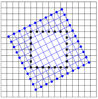
In many problems it is necessary or advantageous to choose coordinate systems adapted to the boundaries. Except for highly symmetric systems, it is often difficult to choose a single coordinate chart appropriate for the entire problem.

A typical case of interest is a spacetime containing a black hole. When black hole excision is used to remove singularities from the computational domain, adapting the boundary to the geometry of the event horizon yields the maximal excision volume. Coordinates adapted to the event horizon or one black hole, however, are usually not appropriate for large domains or for binary black holes. Thus multiple domain numerical techniques are appropriate in numerical relativity using both touching grids [18, 19] and overlapping grids [34, 35, 17, 22, 36]. We concentrate here on overlapping grids.

To test computational techniques for black hole spacetimes, we perform all of the standard flat space tests in this paper on overlapping grids with excision. Figure 1 shows the basic grid configuration used in these tests. The grid ${\cal G}_{1}$ is a base grid from which a square region is excised about the origin, imitating the excision used around a black hole. A second grid, ${\cal G}_{2}$, is placed over the excision region to give the usual simply connected domain required for the flat space tests. ${\cal G}_{2}$ is rotated by an arbitrary angle $\theta$ with respect to ${\cal G}_{1}$. We choose coordinates $(x,y)$ for ${\cal G}_{1}$ and coordinates $(\xi,\eta)$ for ${\cal G}_{2}$, and the coordinates are related by a simple rotation

$$\xi=x\cos\theta+y\sin\theta,\qquad\eta=-x\sin\theta+y\cos\theta.$$ (43)

During the evolution boundary data at the inner boundary of ${\cal G}_{1}$ are obtained by interpolating the solution from ${\cal G}_{2}$. Outer boundary data for ${\cal G}_{2}$ are similarly obtained by interpolating the solution on ${\cal G}_{1}$. For clarity figure 1 indicates these interpolated points in a single row at each boundary. However, our third order evolution scheme requires a seven-point stencil, and we actually interpolate a band of three points at each inter-grid boundary. Finally, interpolation zones between grids are not allowed to overlap.

Conservative variables are interpolated at grid interfaces, although a nonconservative interpolation scheme is used. These variables are typically smoother than the corresponding primitive variables, and have smaller relative jumps near discontinuities. The primitive variables are then recalculated from the interpolated variables. Simple Lagrangian interpolation can lead to oscillatory results near discontinuities, frequently resulting in unphysical states in relativistic fluid dynamics. (This effect may be less pronounced when using structured grids, such for Berger-Oliger AMR.) Therefore we interpolate with WENO interpolation [37], which is designed for use with discontinuous functions. WENO interpolation is summarized in B.

As mentioned briefly above, our FD fluid scheme on overlapping grids with WENO interpolation is not conservative. Conservative systems are often thought to be necessary for obtaining the correct weak solutions to the fluid equations. The effect of non-conservative boundary interpolation on such systems has been examined by Tang and Zhou [38] and Sebastian and Shu [37]. Tang and Zhou found that convergent weak solutions can be obtained using nonconservative interpolation at grid interfaces. Sebastian and Shu found conservation errors of second order at grid interfaces for smooth solutions and first order errors for solutions with discontinuities at the interface. The numerical results presented in this paper are a direct demonstration that we are able to obtain the correct weak solutions when overlapping grids are used.

3.2 CENO

High-Resolution Shock-Capturing (HRSC) methods are designed to solve hyperbolic conservation laws of the form

$$\partial_{t}{\hbox{\bfgreek\char 117\relax}}+\partial_{k}{\hbox{\bfgreek\char 102\relax}}\,^{k}({\hbox{\bfgreek\char 117\relax}})={\hbox{\bfgreek\char 115\relax}}({\hbox{\bfgreek\char 117\relax}}),\qquad{\hbox{\bfgreek\char 117\relax}}(0,x^{i})={\hbox{\bfgreek\char 117\relax}}_{0}(x^{i}),$$ (44)

where u is a state vector, ${{\hbox{\bfgreek\char 102\relax}}}\,^{k}$ are flux functions, and s contains source terms. The semi-discrete discretization in one dimension is

$$\frac{d{\hbox{\bfgreek\char 117\relax}}_{i}}{dt}=-\frac{{\hat{{\hbox{\bfgreek\char 102\relax}}\mkern 8.0mu}\mkern-8.0mu}{}_{i+1/2}-{\hat{{\hbox{\bfgreek\char 102\relax}}\mkern 8.0mu}\mkern-8.0mu}{}_{i-1/2}}{\triangle x}+{\hbox{\bfgreek\char 115\relax}}(u^{i}),$$ (45)

where ${\hat{{\hbox{\bfgreek\char 102\relax}}\mkern 8.0mu}\mkern-8.0mu}{}$ is a consistent numerical flux. The accuracy of the scheme depends, among other things, on the estimation, or reconstruction, of ${\hbox{\bfgreek\char 117\relax}}_{i+1/2}$ from the quantities ${\hbox{\bfgreek\char 117\relax}}_{i-k},\cdots,{\hbox{\bfgreek\char 117\relax}}_{i},\cdots,{\hbox{\bfgreek\char 117\relax}}_{i+m}$, where $k$ and $m$ are integers. TVD schemes are named for the Total Variation Diminishing condition on the interpolating polynomial. These schemes accurately capture the dynamics of strong shocks without oscillations or Gibbs overshoot effects at discontinuities. The TVD condition, however, can also be overly restrictive, reducing the order of accuracy even at smooth extrema.

The Essentially Non-Oscillatory (ENO) philosophy is that the interpolation stencil is chosen based on the local smoothness of the function. All points are used for smooth functions, and thus accuracy is not lost at smooth extrema. Near discontinuities the stencil is locally adjusted to use points away from the discontinuity. In relaxing the TVD condition, small oscillations may develop near discontinuities, but they are of ${\rm O}(\triangle x^{k})$, where $k$ is the order of accuracy. The flexibility of the ENO philosophy has resulted in many extensions, including both FV and FD formulations, the Weighted ENO (WENO) approach, and schemes formally of very high order, etc. Shu reviews the different ENO methods in [14].

The CENO method of Liu and Osher [29] uses a FD discretization and Lax–Friedrichs flux splitting, eliminating the need for a characteristic decomposition. The interpolating polynomial in this scheme is produced by a convex combination of lower order interpolations. Near discontinuities this scheme is designed to produce results similar to TVD methods. This method was modified by Del Zanna and Bucciantini for relativistic fluids [30], and we follow their approach.

We considered three different central or central-upwind numerical fluxes: (1) the Lax–Friedrichs (LF) flux, (2) the local Lax–Friedrichs flux (LLF) and (3) the Harten–Lax–van Leer (HLL) flux. We are primarily interested in highly relativistic systems, where the characteristic speeds approach the speed of light. In this limit the HLL and LLF fluxes reduce to the simple LF flux. Indeed, we have found very little difference between solutions calculated with the LF flux and those calculated with the LLF and HLL fluxes. Similarly, Del Zanna et alalso reported nearly identical results from the LLF and HLL fluxes in this regime [33]. In this paper we use only the LF flux

$${{\hbox{\bfgreek\char 102\relax}}}\,^{\rm LF}_{i+1/2}=\frac{1}{2}\left[{\hbox{\bfgreek\char 102\relax}}({\hbox{\bfgreek\char 117\relax}}^{L}_{i+1/2})+{\hbox{\bfgreek\char 102\relax}}({\hbox{\bfgreek\char 117\relax}}^{R}_{i+1/2})-({\hbox{\bfgreek\char 117\relax}}^{R}_{i+1/2}-{\hbox{\bfgreek\char 117\relax}}^{L}_{i+1/2})\right],$$ (46)

where ${\hbox{\bfgreek\char 117\relax}}^{L}_{i+1/2}$ and ${\hbox{\bfgreek\char 117\relax}}^{R}_{i+1/2}$ are the reconstructed states to the left and right of the interface at $x_{i+1/2}$, respectively. The CENO reconstruction for ${\hbox{\bfgreek\char 117\relax}}^{L}_{i+1/2}$ and ${\hbox{\bfgreek\char 117\relax}}^{R}_{i+1/2}$ is described in A.

In FD ENO fluxes calculated from the point-wise values, ${\hbox{\bfgreek\char 102\relax}}_{i+1/2}$, must be converted into consistent numerical fluxes, ${\hat{{\hbox{\bfgreek\char 102\relax}}\mkern 8.0mu}\mkern-8.0mu}{}_{i+1/2}$. To order $\mbox{O}(\triangle x^{k})$, the conversion from point valued fluxes to conservative fluxes is given by [39, 40]

$${\hat{{\hbox{\bfgreek\char 102\relax}}\mkern 8.0mu}\mkern-8.0mu}{}_{i+1/2}={\hbox{\bfgreek\char 102\relax}}_{i+1/2}+\sum_{j=1}^{(k-1)/2}a_{2j}(\triangle x)^{2j}\left(\frac{\partial^{2j}{\hbox{\bfgreek\char 102\relax}}}{\partial x^{2j}}\right)_{i+1/2},$$ (47)

where $a_{2}=-1/24$ and $a_{4}=7/5760$. For second order schemes the two fluxes are identical, ${\hat{{\hbox{\bfgreek\char 102\relax}}\mkern 8.0mu}\mkern-8.0mu}{}_{i+1/2}={\hbox{\bfgreek\char 102\relax}}_{i+1/2}$. A third order scheme, however, requires the correction

$${\hat{{\hbox{\bfgreek\char 102\relax}}\mkern 8.0mu}\mkern-8.0mu}{}_{i+1/2}=\left(1-\frac{1}{24}{\cal D}^{(2)}\right){\hbox{\bfgreek\char 102\relax}}_{i+1/2},$$ (48)

where ${\cal D}^{(2)}$ is a second-order non-oscillatory difference operator. ${\cal D}^{(2)}f_{i}$ is calculated, again, as a convex combination of the differences

$${\cal D}^{(2)}f_{i}=\mbox{minmod}(\alpha^{-1}D^{(2)}_{-}f_{i},\alpha^{0}D^{(2)}_{0}f_{i},\alpha^{1}D^{(2)}_{+}f_{i}),$$ (49)

where the minmod limiter is

$$\mbox{minmod}(a_{1},a_{2},\cdots)=\left\{\begin{array}[]{ll}\min\{a_{k}\}&\hbox{if all $a_{k}>0$,}\\ \max\{a_{k}\}&\hbox{if all $a_{k}<0$,}\\ 0&\hbox{otherwise,}\end{array}\right.$$ (50)

and the one-sided (first-order) and centered (second-order) second derivative operators are

$$D^{(2)}_{+}f_{i}=f_{i+2}-2f_{i+1}+f_{i},\quad D^{(2)}_{-}f_{i}=f_{i}-2f_{i-1}+f_{i-2},\quad D^{(2)}_{0}f_{i}=f_{i+1}-2f_{i}+f_{i-1}.$$ (51)

The constants $\alpha^{k}$ are weights that may be chosen to bias towards centered differencing. Here we use $\alpha^{-1}=\alpha^{1}=1$ and $\alpha^{0}=0.7$.

3.2.1 Boundary conditions

The third order CENO scheme has a seven point stencil. At physical boundaries three ghost zones are used, which are populated by simple extrapolation. For example, at a boundary $x=x_{0}$ we set $u^{n}_{k,j}=u^{n}_{3,j}$ for $k=0,1,2$ and all $j$. At inter-grid boundaries these ghost zones are set by interpolating from a covering grid using WENO interpolation, as described in B.

3.2.2 Time integration

The semi-discrete equations (45) are integrated in time using third order Runge-Kutta. Various versions of RK3 exist, and we use the optimal third-order scheme of Shu and Osher that preserves the TVD condition [39]

$${\hbox{\bfgreek\char 117\relax}}^{(1)} = {\hbox{\bfgreek\char 117\relax}}^{n}+\triangle tL({\hbox{\bfgreek\char 117\relax}}^{n}),$$

$${\hbox{\bfgreek\char 117\relax}}^{(2)} = \frac{3}{4}{\hbox{\bfgreek\char 117\relax}}^{n}+\frac{1}{4}{\hbox{\bfgreek\char 117\relax}}^{(1)}+\frac{1}{4}\triangle tL({\hbox{\bfgreek\char 117\relax}}^{(1)}),$$ (52)

$${\hbox{\bfgreek\char 117\relax}}^{n+1} = \frac{1}{3}{\hbox{\bfgreek\char 117\relax}}^{n}+\frac{2}{3}{\hbox{\bfgreek\char 117\relax}}^{(2)}+\frac{2}{3}\triangle tL({\hbox{\bfgreek\char 117\relax}}^{(2)}).$$

4 The $\nabla\cdot{\bf B}=0$ constraint

The magnetic field, $\bf B$, must satisfy both its evolution equation as well as the solenoidal constraint: $\nabla\cdot{\bf B}=0$. Small numerical errors lead to violations of this constraint that, experience has shown, can grow rapidly. Left unchecked, violations of this constraint produce unphysical behavior. Various approaches can be used to enforce the solenoidal constraint, and here we consider two that can be applied to domains with multiple arbitrary grids and with a view to incorporating AMR: hyperbolic divergence cleaning and an elliptic projection of $\bf B$. We do not consider constrained transport here because it requires that neighboring grids align in a structured manner, precluding its application to overlapping grids with arbitrary coordinates, resolutions and/or orientations.

4.1 Hyperbolic divergence cleaning

Hyperbolic divergence cleaning is simple to implement numerically and comes with very little computational cost. A new scalar function $\psi$ is added to the system, which can be interpreted as a generalized Lagrange multiplier (GLM), and coupled to the magnetic field equations. The method can be implemented in various ways, and we follow the GLM method of Dedner et al for the classical MHD equations [27]. See van Putten for another approach [41].

We specialize to Cartesian coordinates in flat space, and assume that $\psi$ satisfies a linear differential equation and couples to the magnetic field evolution equation according to

$$\partial_{t}B^{b}+\partial_{i}\left(B^{b}v^{i}-B^{i}v^{b}\right)+g^{bj}\partial_{j}\psi = 0,$$ (53)

$${\cal D}\psi+\nabla\cdot{\bf B} = 0,$$ (54)

where $\cal D$ is a linear differential operator. Various choices for $\cal D$ can be made, giving hyperbolic, parabolic, and elliptic methods for divergence cleaning. We choose

$${\cal D}(\psi)=\frac{1}{c_{h}^{2}}\partial_{t}\psi+\frac{1}{c_{p}^{2}}\psi,$$ (55)

which combines some elements of both hyperbolic and parabolic operators, i.e., both propagating and damping the error. Equation (54) then becomes

$$\partial_{t}\psi+c_{h}^{2}\nabla\cdot{\bf B}=-\frac{c_{h}^{2}}{c_{p}^{2}}\psi.$$ (56)

Differentiating and combining (53)–(54) shows that $\psi$ also satisfies the telegraph equation

$$\partial_{tt}\psi+\frac{c_{h}^{2}}{c_{p}^{2}}\partial_{t}\psi-c^{2}_{h}\nabla^{2}\psi=0.$$ (57)

Violations of the solenoidal constraint propagate with the speed $c_{h}$ and the coefficient $c_{p}$ affects the damping rate.

We have tested hyperbolic divergence cleaning using the cylindrical shock and relativistic rotor problems described below. In our tests we found that hyperbolic divergence cleaning to be very effective at keeping $||\nabla\cdot{\bf B}||_{2}$ bounded during an evolution. Some numerical tests are presented in section 5.4. We turn now to the elliptic projection method.

4.2 The projection method

Blackball and Barnes [42] first proposed an elliptic projection correction to the magnetic field such that it satisfies the constraint $\nabla\cdot{\bf B}=0$. The evolution equations are used to obtain a preliminary estimate for the magnetic field at the advanced time, ${\bf B}^{\star}$. The corrected magnetic field at the advanced time, ${\bf B}^{n+1}$, is then obtained by solving the system

$$\nabla^{2}\psi=\nabla\cdot{\bf B}^{\star},\qquad{\bf B}^{n+1}={\bf B}^{\star}-\nabla\psi.$$ (58)

Tóth has shown for classical MHD that (1) $\nabla\phi$ is the minimal correction to ${\bf B}^{\star}$ that can be made such that $\nabla\cdot{\bf B}^{n+1}=0$, and (2) the projection method gives the correct weak solution [24].

The projection method can be implemented in different ways, e.g., the constraint can be imposed in Fourier space or physical space [25]. We consider here only two different discretizations in physical space. Comparisons of different projection implementations, as well as to other techniques, such as constrained transport, are given by Tóth [24], and Balsara and Kim [25]. The divergence is discretized using the centered discrete operator $D_{0}$, and the Laplacian can be discretized with either $D_{0}D_{0}$ or $D_{+}D_{-}$. In one dimension the operators are

$$(D_{0}v)_{i}=\frac{v_{i+1}-v_{i-1}}{2\triangle x},\qquad(D_{+}D_{-}v)_{i}=\frac{v_{i+1}-2v_{i}+v_{i-1}}{\triangle x^{2}}.$$ (59)

The $D_{0}D_{0}$ operator has a five point stencil in each direction, and the corrected magnetic field exactly satisfies the discrete divergence condition calculated using $D_{0}$. The $D_{+}D_{-}$ operator has a three-point stencil in each direction, and the corrected magnetic field does not exactly satisfy any discrete divergence operator. As noted above, whether or not the magnetic field exactly satisfies a discrete divergence condition is something of a red herring: the continuum solution in both cases is only known to the level of truncation error.

The projection method requires the solution of an elliptic equation (58), which we solve iteratively after each complete Runge-Kutta cycle using a conjugate gradient or stabilized bi-conjugate gradient method. The error tolerance for the elliptic solver is set about 10 times less than the smallest expected truncation error, ${\rm O}(h^{3})$. The solution of the elliptic equations is relatively efficient, requiring about 20–30% of the total run time for typical resolutions. Homogeneous Dirichlet boundary conditions are given for $\psi$ on all physical boundaries. At overlapping grid boundaries $\psi$ is interpolated as with other variables.

When large corrections to ${\bf B}^{\star}$ are made in the projection process, problems can arise in reconstructing the corrected primitive variables. This may occur because both $S_{a}$ and $\tau$ are themselves functions of the magnetic field, c.f. (36). We compensate by also “correcting” these variables after projecting $\bf B$, slightly modifying the conventional correction used in classical MHD [24]. The projection algorithm can thus be summarized by

1. Solve the evolution equations for preliminary values at the advanced time ${\hbox{\bfgreek\char 117\relax}}^{\star}$;

2. From ${\hbox{\bfgreek\char 117\relax}}^{\star}$ calculate the primitive variables at the advanced time ${\hbox{\bfgreek\char 119\relax}}^{n+1}({\hbox{\bfgreek\char 117\relax}}^{\star})$;

3. Solve (58) for $\psi$ and compute ${\bf B}^{n+1}$;

4. Recalculate ${\hbox{\bfgreek\char 117\relax}}^{n+1}$ from ${\hbox{\bfgreek\char 119\relax}}^{n+1}$ and ${\bf B}^{n+1}$.

This method assumes that the primitive variables more accurately reflect the correct solution in the projection process. Again, this is because $\rho$, $v^{a}$, and $P$ are not functions of the magnetic field, whereas the conserved variables $S^{a}$ and $\tau$ are functions of ${\bf B}$.

5 Test Problems

This section presents numerical results of our CENO scheme on overlapping grids. The first tests are a set of standard Riemann problem tests for relativistic MHD proposed by Komissarov [43, 44]. Although these tests are inherently one dimensional problems, we run them on unaligned overlapping grids, making them effectively two dimensional problems. This allows us to test our divergence cleaning and interpolation methods on known solutions. We then discuss two test problems that are naturally two dimensional, the cylindrical shock and relativistic rotor problems described by Del Zanna et al [33]. Finally we present comparisons of the different divergence cleaning methods.

5.1 Riemann problem tests

Figure 2: This figure shows four Komissarov test problems. Solutions calculated on two-dimensional overlapping grids with elliptic divergence cleaning (plotted along the line $y=0$) are compared with the one-dimensional solutions. The solutions are nearly indistinguishable. From left to right, top to bottom, these problems are: (1) Slow Shock, (2) Switch-off Fast Rarefaction, (3) Switch-on Slow Rarefaction, and (4) Compound Wave. Triangles indicate the solution on the excised base grid, ${\cal G}_{1}$, and crosses indicate the solution on a grid covering the excision region, ${\cal G}_{2}$, rotated 45^∘ with respect to the base grid. Solid lines indicate the single-grid solution, and not the exact solution.

Figure 3: This figure shows two Komissarov test problems calculated on overlapping grids. The left frame shows Shock Tube # 1 and the right frame is Shock Tube # 2. See the caption to figure 2 for further explanation.

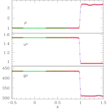
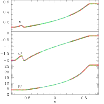
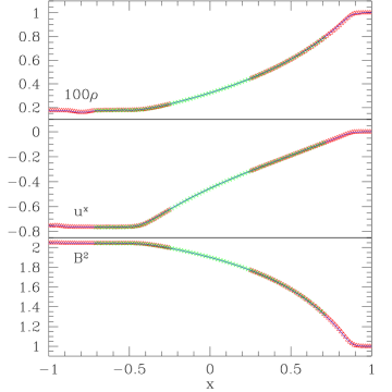
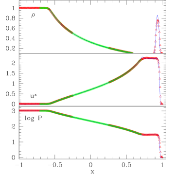
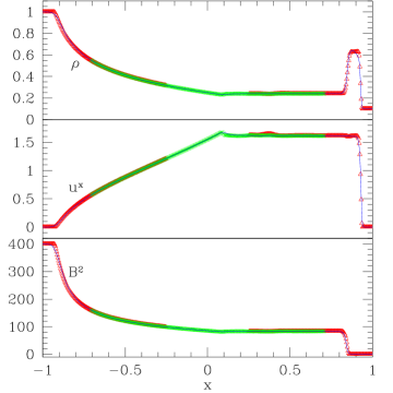
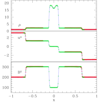
Solutions of the Riemann problem are used to test shock capturing numerical methods, allowing one to verify that a method faithfully produces the fundamental shock, rarefaction and, for MHD, Alfven waves. The analytic solution of the relativistic MHD Riemann problem is given by Giacomazzo and Rezzolla [45]. Komissarov presented several Riemann problem tests for RMHD, which we have used to test our code [43, 44]. For comparison, results for Komissarov’s tests have also been published by other researchers [33, 12, 13]. With the initial discontinuity aligned with a coordinate direction, we are able to successfully reproduce all of Komissarov’s test problems, though we have reduced the Courant number to $\lambda=0.4$ in all tests, possibly because we are using the more diffusive Lax–Friedrichs flux.

When the discontinuity is rotated with respect to the coordinates, we are able to run all Komissarov tests but two, the Fast Shock and the Collision. This problem occurs even when using a single computational grid, and thus is not related to using overlapping grids. In both cases we calculate unphysical values for the primitive variables, and the code is immediately halted before the solution is completed. We do not consider the Fast Shock problem here, and have modified the Collision problem by reducing the initial velocities from $\pm 0.981$ to $\pm 0.951$.

To provide the most comprehensive test of our algorithm, the Riemann problem tests presented here are performed on unaligned overlapping grids with excision. Excision is used here somewhat unconventionally, as the entire computational domain is simply connected. However, these Riemann problems can be used to test the excision and divergence cleaning algorithms. For example, we test that unphysical effects do not arise as waves pass through grid interfaces, and that the divergence cleaning methods do not adversely affect the solution. These solutions are then compared with those obtained from a single grid aligned to the initial discontinuity, with no excision and where divergence cleaning is unnecessary. Results from these tests are presented in Figures 2 and 3.

In all tests $\Gamma=4/3$, the Courant factor is $\lambda=0.4$, and elliptic divergence cleaning is used. Second order reconstruction with the minmod limiter is used in all tests except the collision problem, where first order reconstruction is more appropriate. The initial discontinuity in the fluid data is aligned with the coordinates $(x,y)$ of a base grid, ${\cal G}_{1}$. The region $(x,y)\in[-\frac{1}{4},\frac{1}{4}]$ is excised from ${\cal G}_{1}$, and a second grid, ${\cal G}_{2}$, covers this excision region to form the complete computational domain. ${\cal G}_{2}$ has coordinates $(\xi,\eta)\in[-\frac{1}{2},\frac{1}{2}]$, which are related to $(x,y)$ by a rotation of angle $\theta$ about the origin (43). We choose $\theta=45^{\circ}$ for simplicity in plotting the results of our runs. In Figures 2 and 3 we plot data from the line $y=0$ for ${\cal G}_{1}$ and the diagonal elements of ${\cal G}_{2}$.

In all cases we see that the solutions calculated on overlapping grids are nearly indistinguishable from those calculated on the single grid. In particular, we do not see reflections from the grid boundaries. Ill effects from elliptic divergence cleaning are also not observed in comparison to the single grid runs, where divergence cleaning is not used.

5.2 Cylindrical blast wave

Figure 4: This figure shows solutions of the cylindrical shock and relativistic rotor test problems at $t=0.4$. The top two frames show $P$ and $B^{2}$ for the cylindrical shock problem, and the bottom two frames show the same variables for the relativistic rotor problem. Details about the evolutions are given in the text.

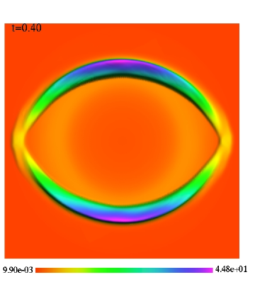
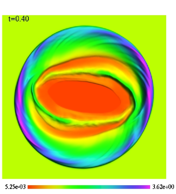
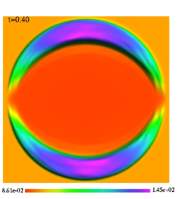
Del Zanna et alpresented this cylindrical shock test problem for relativistic MHD [33]. The initial data consist of a uniform fluid background with $\rho=1$, $P=0.01$, ${\bf v}=(0,0,0)$ and ${\bf B}=(4,0,0)$. Inside a disk of radius $0.16$ centered at the origin, we set $P=1000$. The adiabatic index is $\Gamma=4/3$. An analytic solution is not available, but comparisons can be made with other published results [33, 13]

The solution is calculated using two overlapping grids with an excised region in the base grid. The base grid is uniform with $(x,y)\in[-1,1]$, excluding the region $(x,y)\in[-0.2,0.2]$. The resolution is $h=0.008$. A second grid covers the excision region with coordinates $(\xi,\eta)\in[-0.34,0.34]$, rotated $50^{\circ}$ with respect to the base grid.

Figure 4 shows $P$ and $B^{2}$ at $t=0.4$. The solution is calculated using second order reconstruction, with a Courant number of $\lambda=0.2$, and elliptic divergence cleaning. The Courant number is lower than that used by Del Zanna et al, which may be a consequence of a different numerical flux and using a grid, ${\cal G}_{2}$, rotated with respect to the initial magnetic field. The pressure difference is initially very large, leading to a strong out-going shock. The initially circular shock becomes distorted through interaction with the magnetic field, giving the elliptical profile observed in the figure. Comparing these results with those of other researchers, no artificial grid effects are observed in the solution, which could arise from using excision and overlapping grids.

5.3 Relativistic rotor

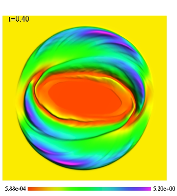
A second two-dimensional MHD test is the relativistic rotor, which evolves an initially rigidly rotating fluid in the presence of a magnetic field [33]. Initial data consist of a constant background state with $\rho=1$, $P=1$, ${\bf v}=(0,0,0)$ and ${\bf B}=(1,0,0)$. Inside a disk of radius $0.1$ at the center of the domain, the density is $\rho=10$, and the fluid is rigidly rotated with $\omega=9.95$. The linear velocity at the edge of the disk is $0.995$ and $W=10$. Finally, the adiabatic index is $\Gamma=5/3$.

The solution is calculated using two overlapping grids. The first grid has coordinates $(x,y)\in[-1/2,1/2]$, excluding the region $(x,y)\in[-0.13,0.13]$. A second grid covers the excision region, and is rotated $27^{\circ}$ with respect to the first grid. This grid has coordinates $(\xi,\eta)\in[-0.2,0.2]$. The resolution on both grids is $h=0.0025$. Figure 4 shows $P$ and $B^{2}$ at $t=0.4$. The Courant factor is $\lambda=0.2$, and second order reconstruction and elliptic divergence cleaning are used. Again, these results appear very similar to other published solutions, and no artificial grid effects are observed.

5.4 Divergence Cleaning

Figure 5: This figure compares the hyperbolic and elliptic divergence cleaning methods in two different cylindrical shock problems. Each figure plots the L2 norm of $\nabla\cdot{\bf B}$ as a function of time for a free evolution, an evolution using hyperbolic divergence cleaning, and elliptic divergence cleaning using both $D_{+}D_{-}$ and $D_{0}D_{0}$ operators. Initial data for the left frame have a central pressure $P_{c}=10$ and the central pressure for the right frame is $P_{c}=1000$. Unfortunately, these L2 norms are dominated by a few points primarily near shocks, but this gives some indication of how violations of the constraint vary in time.

Figure 6: This figure shows the distribution of $|\nabla\cdot{\bf B}|$ at an instant of time, $t=0.36$, for the cylindrical shock problem with $P_{c}=1000$. On a given grid, the number of points, $N$, with $|\nabla\cdot{\bf B}|$ in a specified range are counted, and $\log_{10}(1+N)$ is plotted on the vertical axis. The total number of points is $501^{2}$. In the left frame the solid line corresponds to the free evolution, the dotted line an evolution with hyperbolic divergence cleaning, and the dashed line corresponds to elliptic divergence cleaning with the three-point stencil. In the right frame, the lines are ordered from top to bottom: free evolution, hyperbolic divergence cleaning, three-point elliptic divergence cleaning. Points with $|\nabla\cdot{\bf B}|<10^{-11}$ were excluded from the distribution on the left.

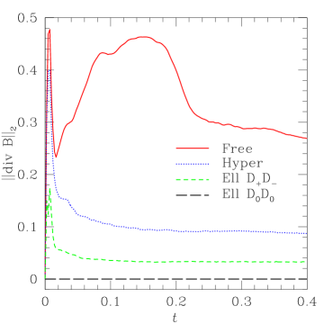
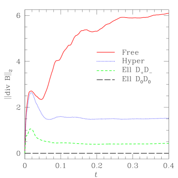
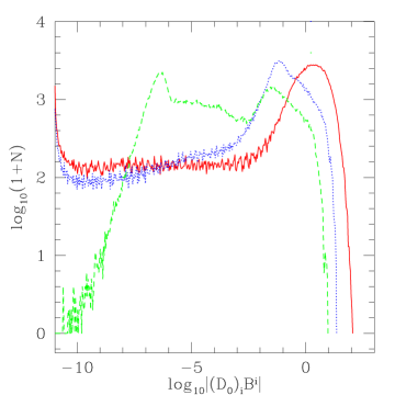
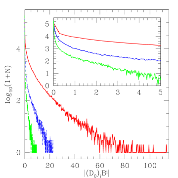
This section presents numerical results comparing the divergence cleaning techniques discussed in section 4. We slightly modify the cylindrical shock problem of section 5.2, and monitor $\nabla\cdot{\bf B}$ during the subsequent evolution for (1) a free evolution (no divergence cleaning), (2) an evolution with hyperbolic divergence cleaning, and (3) elliptic divergence cleaning evolutions with $D_{+}D_{-}$ and $D_{0}D_{0}$ discrete divergence operators.

The cylindrical shock problem is modified by changing the background pressure to $P=1$, and varying the central pressure, $P_{c}$. In the examples presented here, the central pressure is $P_{c}=10$ and $P_{c}=1000$. We examined other values of $P_{c}$, but the results were essentially the same as in these two cases. (The differences arise only in the overall scale of the constraint violation, not in the relative performance of each technique.) The evolutions are performed on a single grid with $501^{2}$ points with coordinates $(x,y)\in[-\frac{1}{2},\frac{1}{2}]$. During the evolutions $\nabla\cdot{\bf B}$ is calculated using the central discrete operator $D_{0}$. To emphasize the discrete nature of these calculations, we write the numerically calculated divergences as $(D_{0})_{i}B^{i}$.

Comparing the divergence cleaning techniques is more difficult than it appears at first blush. The first impulse is to simply plot L2 norms of $(D_{0})_{i}B^{i}$ as a function of time, as shown in figure 5. Glancing quickly at this figure, one might conclude that the elliptic divergence cleaning with $D_{0}D_{0}$ gives ideal results, as $||(D_{0})_{i}B^{i}||_{2}$ can be made as small as desired. However, as discussed previously, “exact” satisfaction of the constant can be a red herring, in that it does not imply that the continuum constraint is “exactly” satisfied. Using the same elliptic projection method with a different discrete divergence operator, the $D_{+}D_{-}$ operator, gives a non-zero value for $||(D_{0})_{i}B^{i}||_{2}$ and a better indication of error in the solution.

A second difficulty is that the largest constraint violations appear, not surprisingly, near shocks. Indeed, examination of the data show that a few points near the shock completely dominate the values of $||(D_{0})_{i}B^{i}||_{2}$. This makes the comparison of L2 norms in figure 5 problematic, as they provide almost no information about constraint violations in smooth parts of the solutions, where comparisons between techniques may be more meaningful. Moreover, since convergence in the sense of Richardson extrapolation can not be defined for discontinuous solutions, the norms $||(D_{0})_{i}B^{i}||_{2}$ do not become smaller with finer resolution, rather, the opposite occurs. With finer resolution, the shock profile is sharpened, and derivatives of the discontinuous variable approach the continuum derivative: $d/dx[\theta(x-x^{\prime})]=\delta(x-x^{\prime})$. Ideally one could remove points near the shock from the comparisons, by either tracking the shocks or simply removing points where $|(D_{0})_{i}B^{i}|$ is judged to be too large. We have no facility for the former, and the latter strikes us as too arbitrary. Since L2 norms of $(D_{0})_{i}B^{i}$ give at best limited information, in figure 6 we plot the distribution of $|(D_{0})_{i}B^{i}|$ at a single instance of time for the cylindrical shock problem with $P_{c}=1000$.

6 Conclusion

The numerical scheme presented here is for solving the relativistic MHD equations on multiple domains with overlapping grids. While we have not presented data from black hole spacetimes in this paper, it is the target application that has influenced our design decisions. First, we choose to work with multiple domains since excision is most naturally implemented with smooth boundaries adapted to the event horizon’s geometry. The flexibility of the overlapping grid approach allows one to easily use high resolution shock-capturing schemes on multiple domains.

Secondly, we choose an ENO method with a finite difference discretization to simplify the transfer of information from one grid to another. While a conservative scheme for overlapping grids could be used [46], working with point values instead of cell averages simplifies the interpolation process for arbitrary grids. ENO finite difference schemes are also easily extended to higher dimensions and higher orders of accuracy.

Thirdly, we choose a central scheme to solve the RMHD equations. Central schemes are very efficient HRSC methods, and ideal for combining with AMR to resolve small features.

Fourth, we investigated the use of hyperbolic and elliptic divergence cleaning to maintain the $\nabla\cdot{\bf B}=0$ constraint for MHD. These techniques are readily used on domains with arbitrary overlapping grids. We found that hyperbolic divergence cleaning often gives acceptable results, especially for moderate shocks. Elliptic divergence cleaning is more robust, but also more more computationally expensive.

Finally, it is natural to use a finite difference formulation of the fluid equations when also solving the finite difference Einstein equations with AMR. When both the fluid and geometric variables are refined in the same manner, the inconvenience of using staggered grids with AMR is eliminated.

Appendix A CENO Reconstruction

This appendix summarizes the CENO reconstruction scheme used by Del Zanna, Bucciantini and Londrillo [30, 33], based on the original scheme of Liu and Osher [29]. The numerical fluxes are constructed dimension by dimension, thus the basic algorithm is one dimensional. Consider an uniform grid $x_{i}=i\triangle x$ with the function $v_{i}=v(x_{i})$. The standard one-sided and centered discrete differential operators are

$$(D_{\pm}v)_{i}=\pm\frac{v_{i\pm 1}-v_{i}}{\triangle x},\qquad(D_{0}v)_{i}=\frac{v_{i+1}-v_{i-1}}{2\triangle x}.$$ (60)

To reconstruct $v_{i}$ on the interval $[x_{i-1/2},x_{i+1/2}]$ we first create a linear TVD interpolating polynomial

$$v^{(1)}_{i}=v_{i}+v_{i}^{\prime}(x-x_{i}),$$ (61)

where $v_{i}^{\prime}$ is the limited slope at $x_{i}$. $v_{i}^{\prime}$ is

$$v^{\prime}_{i}=\mbox{minmod}(D_{-}v_{i},D_{+}v_{i}).$$ (62)

where the minmod limiter is defined in (50). Other TVD limiters can be considered, such as the monotonized central difference limiter, but we do not consider them here. The first order reconstruction is $v(x)=v^{(1)}(x)$, which is equivalent to the TVD reconstruction, and results in a second-order scheme.

Higher order reconstructions proceed hierarchically using the ENO philosophy of constructing multiple candidate polynomials, and then choosing the polynomial that is closest to the lower order polynomial. For example three candidate quadratic polynomials, $Q^{k}_{i}(x)$, $k=-1,0,1$, for a second order reconstruction are

$$Q^{k}_{i}(x)=v_{i+k}+D_{0}v_{i+k}(x-x_{i+k})+\frac{1}{2}D_{+}D_{-}v_{i+k}(x-x_{i+k})^{2}.$$ (63)

These second order polynomials are compared to the first order polynomial at the point of interest, $x$, to calculate the weighted differences

$$d^{k}(x)=\alpha^{k}\left(Q^{k}_{i}(x)-v^{(1)}(x)\right).$$ (64)

The weights $\alpha^{k}$ are chosen to be $\alpha^{-1}=\alpha^{1}=1$ and $\alpha^{0}=0.7$, biasing the interpolation towards the centered polynomial. When all $d^{k}$ have the same sign, the second order reconstruction is $v(x)=Q^{\alpha}_{i}(x)$, where $\alpha$ is the index corresponding to the weighted difference with the smallest magnitude, $d^{\alpha}(x)=\mbox{min}(|d_{k}(x)|)$. When $d_{k}(x)$ have differing signs, we revert to a first order reconstruction, $v(x)=v^{(1)}(x)$. This comparison to the first order reconstruction yields results similar to TVD schemes near discontinuities, but gives an higher order reconstruction for smooth functions.

Appendix B WENO interpolation

Figure 7: A five point interpolation stencil is divided into three substencils, $S_{0}$, $S_{1}$ and $S_{2}$, each with three points. Interpolants are calculated using all three stencils, which are then combined in a weighted convex sum. The nonlinear weights depend on the smoothness of the function.

Boundary data at interfaces between overlapping grids are obtained by interpolation. Following Sebastian and Shu [37], we have investigated both Lagrangian and WENO interpolation at these grid interfaces. Lagrangian interpolating polynomials work well for smooth functions. Near discontinuities, however, they become oscillatory, which can lead to unphysical states in relativistic MHD, i.e., physical primitive variables can not be obtained from the interpolated conservative variables. WENO interpolation avoids these oscillations near discontinuities by adjusting the interpolation stencil according to the local smoothness of the data. The WENO interpolant is constructed as a convex sum of lower order interpolations computed on substencils. The contribution from each substencil is weighted nonlinearly by measures of the function’s local smoothness. For smooth functions, WENO interpolation closely approximates Lagrangian interpolation. A lower-order interpolant is calculated near discontinuities, which is biased towards substencils where the function is smooth. In this appendix we summarize the WENO interpolation algorithm [37] that we use exclusively in our code.

Consider a discrete function $u_{i}$ defined at $(2k-1)$ points, $x_{i}$, $i=0,\ldots,2k-2$. The Lagrangian interpolation polynomial $u_{L}(x)$ is

$$u_{L}(x)=\sum_{i=0}^{2k-2}c_{i}(x)u_{i},\qquad c_{i}(x)=\prod_{j=0}^{2k-2}\frac{x-x_{j}}{x_{i}-x_{j}}.$$ (65)

To motivate WENO interpolation, we divide the $(2k-1)$ points into $k$ substencils, see figure 7, and write $u_{L}(x)$ as a sum of lower order interpolating polynomials on each substencil. Let the substencils be $S_{r}(i)=\{x_{i-r},\ldots,x_{i-r+k-1}\}$ for $r=0,\ldots,k-1$. The Lagrangian interpolating polynomial on each substencil is

$$u^{(r)}_{L}(x)=\sum_{j=0}^{k-1}u_{i-r+j}c_{rj}(x),\qquad c_{rj}(x)=\prod_{\ell=0,\ell\neq j}^{k-1}\frac{x-x_{i-r+\ell}}{x_{i-r+j}-x_{i-r+\ell}}.$$ (66)

We can expand $u_{L}(x)$ in terms of $u^{(r)}_{L}(x)$ as

$$u_{L}(x)=\sum_{r=0}^{k-1}d_{r}(x)u^{(r)}_{L}(x),$$ (67)

where $d_{r}(x)$ are constants, or linear weights, that depend on $x$. Consistency requires that $\sum_{r=0}^{k-1}d_{r}(x)=1.$

The Lagrangian interpolation polynomial $u_{L}(x)$ is written above as a sum of lower-order polynomials in (67). WENO interpolation generalizes this by creating a convex sum, where the weights are nonlinearly dependent on the local smoothness of $u_{i}$. The WENO interpolation polynomial has the form

$$u_{w}(x)=\sum_{r=0}^{k-1}\omega_{r}(x)u^{(r)}_{L}(x)$$ (68)

where $\omega_{r}(x)$ are the nonlinear weights, and for consistency we require $\sum_{r=0}^{k-1}\omega_{r}(x)=1.$ Following the fundamental reconstruction procedure for WENO evolution schemes, the weights are chosen to be

$$\omega_{r}(x)=\frac{\tilde{\omega}_{r}(x)}{\sum_{s=0}^{k-1}\tilde{\omega}_{s}(x)},\qquad\tilde{\omega}_{r}(x)=\frac{d_{r}(x)}{(\varepsilon+\beta_{r}(x))^{2}},$$ (69)

where $\varepsilon$ is a small number that we set as $\varepsilon=10^{-6}$. The coefficients $d_{r}(x)$ are obtained from (67), and the functions $\beta_{r}(x)$ are smoothness indicators given by

$$\beta_{r}(x)=\sum_{\ell=1}^{k-1}\int_{a}^{b}\triangle x^{2\ell-1}\left(\frac{d^{\ell}}{dx^{\ell}}u^{(r)}_{L}(x)\right)^{2}\,{\rm d}x,$$ (70)

where the limits of integration are over different substencils. All interpolations for the grids used in this paper are centered, $x\in[x_{i-1/2},x_{i+1/2}]$. In this case the smoothness indicators become [37]

$$\beta_{0} = (10u_{i}^{2}-31u_{i}u_{i+1}+25u_{i+1}^{2}+11u_{i}u_{i+2}-19u_{i+1}u_{i+2}+4u_{i+2}^{2})/3$$ (71)

$$\beta_{1} = (4u_{i-1}^{2}-13u_{i-1}iu_{i}+13u_{i}^{2}+5u_{i-1}u_{i+1}-13u_{i}u_{i+1}+4u_{i+1}^{2})/3$$ (72)

$$\beta_{2} = (4u_{i-2}^{2}-19u_{i-2}u_{i-1}+25u_{i-1}^{2}+11u_{i-2}u_{i}-31u_{i-1}u_{i}+10u_{i}^{2})/3$$ (73)

Figure 8: Interpolations in two dimensions are calculated as a series of one dimensional interpolations. The dashed diagonal lines represent coordinate lines for a grid that requires interpolated at their intersection, indicated by the solid circle. The interpolation data are calculated from the grid with rectangular coordinate lines by first interpolating horizontally, using the points indicated by open circles, to obtain data at the points indicated by solid squares. The stencil indicated by solid squares is then used to obtain interpolation data at the required point.

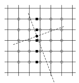
Since the interpolation coefficients $\omega_{r}(x)$ depend on the smoothness of the function, they must be calculated for each function individually, whereas Lagrangian interpolation coefficients are only position dependent. This makes WENO interpolation more expensive to implement when several functions must be interpolated at a single point. Finally, Interpolations in two dimensions are calculated as a series of one dimensional WENO interpolations, as shown in figure 8.

References

- [1] Blandford R D and Znayek R L 1977 MNRAS 179 433
- [2] Balbus S A and Hawley J F 1991 Astrophys. J. 376 214
- [3] Arnowitt R, Deser S and Misner C 1962 Gravitation: An Introduction to Current Research, ed L Witten (New York: Wiley)
- [4] Sloan J and Smarr L L 1985 Numerical Astrophysics ed J L J Centrella et al(Boston: Jones and Bartlett) p 52
- [5] Evans C R and Hawley J F 1988 Astrophys. J. 332 659
- [6] Koide S, Meier D L, Shibata K and Kudoh T 2000 Astrophys. J. 536 668
- [7] De Villiers J-P and Hawley J F 2002 arXiv:astro-ph/0210518
- [8] Gammie C F, McKinney J C and Tóth G 2003 Astrophys. J. 589 444
- [9] Baumgarte T W and Shapiro S L 2003 Astrophys. J. 585 930
- [10] Komissarov S S 2004 MNRAS 350 1431
- [11] Anton L Zanotti O Miralles J A, Marti J M, Ibanez J M, Font J A and Pons J A 2005 Numerical 3+1 general relativistic magnetohydrodynamics: a local characteristic approach Preprint astro-ph/0506063
- [12] Duez M D, Liu Y T, Shapiro S L and Stephens B C 2005 Relativistic Magnetohydrodynamics In Dynamical Spacetimes: Numerical Methods And Tests Preprint astro-ph/0503420.
- [13] Shibata M and Sekiguchi Y I 2005 Phys. Rev.D 72 044014
- [14] Shu C-W 1997 ICASE Report 97-65, NASA Langley Research Center
- [15] Scheel M 2000 Miniprogram on Colliding Black Holes: Mathematical Issues in Numerical Relativity, Institute for Theoretical Physics, University of California at Santa Barbara, January 10–28 2000. Available online at http://online.kitp.ucsb.edu/online/numrel00
- [16] Lehner L, Neilsen D, Reula O and Tiglio M 2004 Class. Quantum Grav.bf 21 5819
- [17] Calabrese G and Neilsen D 2004 Phys. Rev.D 69 044020
- [18] Kidder L E, Scheel M A, Teukolsky S A, Carlson E D and Cook G B 2000 Phys. Rev.D 62 084032
- [19] Lehner L, Reula O and Tiglio M 2005 Class. Quantum Grav.22 5283
- [20] Starius G 1980 Numer. Math. 35 241
- [21] Chessire G and Henshaw W D 1990 J. Comput. Phys. 90 1
- [22] Calabrese G and Neilsen D 2005 Phys. Rev.D 71 124027
- [23] Lehner L and Reula O 2005 Personal communication
- [24] Tóth G 2000 J. Comput. Phys. 161 605
- [25] Balsara D S and Kim J S 2004 Astrophys. J. 602 1079
- [26] Balsara D 2001 J. Comput. Phys. 174 614
- [27] Dedner A, Kemm F, Kröner D, Munz C-D, Schnitzer T and Wesenberg M 2002 J. Comput. Phys. 175 645
- [28] Brodbeck O, Frittelli S, Hubner P and Reula O A 1999 J. Math. Phys. 40 909
- [29] Liu X-D and Osher S 1998 J. Comput. Phys. 142 304
- [30] Del Zanna L and Bucciantini N 2002 Astron. Astrophys. 390 1177
- [31] Lucas-Serrano A, Font J A, Ibanez J M and Marti J M 2004 Assessment of a high-resolution central scheme for the solution of the relativistic hydrodynamics equations Preprint astro-ph/0407541
- [32] Shibata M and Font J A 2005 Phys. Rev.D 72 047501
- [33] Del Zanna L, Bucciantini N and Londrillo P 2003 Astron. Astrophys. 400 397
- [34] Thornburg J 2000 A multiple-grid-patch evolution scheme for 3-D black hole excision Preprint gr-qc/0012012
- [35] Thornburg J 2003 AIP Conf. Proc. 686 247
- [36] Thornburg J 2004 Class. Quantum Grav.21 3665
- [37] Sebastian K and Shu C-W 2003 SIAM J. Sci. Comput. 19 405
- [38] Tang H S and Zhou T, SIAM J. Numer. Anal. 37 173
- [39] Shu C-W and Osher S 1988 J. Comput. Phys. 77 439
- [40] Shu C-W and Osher S 1989 J. Comput. Phys. 83 32
- [41] van Putten M H P M 2002 J. Math. Phys. 43 6195
- [42] Brackbill J U and Barnes D C 1980 J. Comp. Phys. 35 426
- [43] Komissarov S S 2002 Test problems for relativistic magnetohydrodynamics Preprint astro-ph/0209213
- [44] Komissarov S S 1999 Mon. Not. Roy. Astron. Soc. 303 343
- [45] Giacomazzo B and Rezzolla L 2005 The Exact Solution of the Riemann Problem in Relativistic MHD Preprint gr-qc/0507102
- [46] Liu Y 2005 J. Comp. Phys. 209 82