Bifurcation and fine structure phenomena in critical collapse of a self-gravitating $\sigma$-field

Abstract

Building on previous work on the critical behavior in gravitational collapse of the self-gravitating $SU(2)$ $\sigma$-field and using high precision numerical methods we uncover a fine structure hidden in a narrow window of parameter space. We argue that this numerical finding has a natural explanation within a dynamical system framework of critical collapse.

Introduction

Over the past few years the Einstein–$SU(2)\!-\!\sigma$ model has attracted a great deal of attention w1 ; bw1 ; ch ; w2 ; bw2 ; bsw ; s . This model is interesting because its rich phenomenology is sensitive to the value of a dimensionless parameter $\eta$ which leads to various bifurcation phenomena. The most interesting bifurcation was found by Lechner et al. w2 who showed that the critical behavior in gravitational collapse changes character from continuous to discrete self-similarity when the coupling constant $\eta$ increases above a critical value $\eta_{c}$. This phenomenon was interpreted in terms of dynamical systems theory as the homoclinic loop bifurcation where the two critical solutions, continously self-similar (CSS) and discretely self-similar (DSS), merge in phase space. Since the echoing period $\Delta$ of the DSS solution diverges as $\eta\rightarrow\eta_{c}$, the numerical analysis of this bifurcation is extremely difficult and for this reason some of the aspects of critical behavior near the bifurcation point, in particular the black hole mass scaling law, were left open in w2 .

Below, using high precision numerical methods, we confirm the main findings of w2 . In addition, we find that just above the bifurcation point the marginally supercritical side of the transition between dispersion and black holes exhibits a fine structure which is due to the competition between two coexisting critical solutions, the DSS one and the CSS one. The description of this phenomenon and its interpretation is the main purpose of this paper. The rest of the paper is organized as follows. For readers’ convenience, in section 2 we first briefly repeat the basic setting of the model and then we summarize what is known about it. In section 3 we present numerical results and finally, in section 4, we interpret them.

The model

The spherically symmetric Einstein-$SU(2)-\sigma$ system is parametrized by three functions: the metric coefficients $A(t,r)$, $\delta(t,r)$ and the $\sigma$-field $F(t,r)$, which satisfy the following system of equations

$$\Box_{g}F-\frac{\sin(2F)}{r^{2}}=0,\quad\Box_{g}=-e^{\delta}\partial_{t}(e^{\delta}A^{-1}\partial_{t})+\frac{e^{\delta}}{r^{2}}\partial_{r}(r^{2}e^{-\delta}A\>\partial_{r}),$$ (1)

$${\partial_{t}A} = -2\eta\>rA(\partial_{t}F)(\partial_{r}F),$$ (2)

$${\partial_{r}\delta} = -\eta\>r\left((\partial_{r}F)^{2}+A^{-2}e^{2\delta}(\partial_{t}F)^{2}\right),$$ (3)

$$\partial_{r}A = \frac{1-A}{r}-\eta\>r\left(A(\partial_{r}F)^{2}+A^{-1}e^{2\delta}(\partial_{t}F)^{2}+2\>\frac{\sin^{2}{\!F}}{r^{2}}\right),$$ (4)

where $\eta$ is a dimensionless coupling constant. For $\eta=0$ this system reduces to the $\sigma$ model in Minkowski spacetime. The initial value problem for this system was studied by Bizoń et al. bct for $\eta=0$ and by Husa et al. w1 for $\eta>0$. In these studies an important role is played by self-similar solutions. A countable family of continuously self-similar (CSS) solutions, herefater denoted by $CSS_{n}$ ($n=0,1,...$), was shown to exist for $0\leq\eta<0.5$ in b1 ; bw1 ; bw2 . These solutions are regular within the past light cone of the singularity, however they have a spacelike hypersurface of marginally trapped surfaces, i.e. an apparent horizon outside the past light cone if $\eta>\eta_{n}$, where $\eta_{n}$ is an increasing sequence ($\eta_{0}=0.08$, $\eta_{1}=0.152$, etc.). Linear stability analysis shows that the ”ground state” $CSS_{0}$ is stable while the excitations $CSS_{n}$ have exactly $n$ unstable modes.

Besides the CSS solutions, the system (1-4) has also a discretely self-similar (DSS) solution for $\eta\geq\eta_{c}\approx 0.17$. This solution was constructed by Lechner ch via a pseudospectral method following the lines of Gundlach g .

Next, we summarize what is known about the critical behavior in gravitational collapse in this model. The first numerical studies of this problem, reported in w1 , focused on relatively large coupling constants $\eta>0.2$. In this range a ”clean” type II critical DSS behavior was observed, however the attempts to resolve critical evolutions for lower values of $\eta$ encountered numerical difficulties and for $0.18<\eta<0.2$ only an approximate DSS behavior was observed. Furthermore the echoing period $\Delta$ was found to increase sharply as the coupling constant decreases from 0.5 to 0.18. The critical behavior for smaller couplings $0.1<\eta<0.2$ was studied in w2 (still smaller couplings are less interesting because then the model admits naked singularities). In the range $0.1<\eta<0.14$ a ”clean” CSS critical behavior was observed, thus it became clear that somewhere in the interval $0.14<\eta<0.2$ there must be a transition between CSS and DSS critical solutions. The detailed studies of this transition w2 led to a conjecture that there exist a critical value of the coupling constant $\eta_{c}\approx 0.17$ for which the system exhibits the homoclinic loop bifurcation, i.e. the CSS saddle merges with the DSS limit cycle in the phase space. These results left open the question which of the two solutions in the transition region acts as the critical solution at the threshold of black hole formation. In particular, near the bifurcation point the black-hole mass scaling could not be properly resolved.

Numerical results

We have solved equations (1)-(4) for marginally critical initial data fine tuned to the DSS solution for coupling constants close to the critical value $\eta_{c}=0.17$. Since the echoing period $\Delta$ increases sharply as the coupling constant tends to its critical value from above, it becomes more and more difficult to follow the evolution over a large number of DSS cycles. We used the fully constrained implicit evolution scheme based on the Newton-Raphson iteration. In order to resolve the singular behavior near the origin we used the grid which is uniform in $\ln(r)$. To get several cycles of the DSS attractor near the bifurcation point we had to fine tune parameters of initial data with precision of $70$ digits - this was achieved with the help of the arprec library arp

Actually, it was not our aim to determine $\Delta$ with high precision, but rather to show that there exists a $\Delta$ to which the evolution converges. To this end, we determine $\Delta$ as a function of time (cycles) as the evolution approaches the limit cycle i.e. the DSS solution. For a marginally critical solution we plot the function $F$ versus $\ln(r)$ for some late time $t_{1}$ and superimpose the profile of the first echo at time $t_{2}$ shifted by $\ln(r)\rightarrow\ln(r)+\Delta_{r}$. The time $t_{2}$ and the radial echoing period $\Delta_{r}$ are chosen to minimize the discrepancy between two profiles. We also define the temporal echoing period $\Delta_{t}$ by the formula $t_{2}=t^{*}(1-e^{-\Delta_{t}})+e^{-\Delta_{t}}t_{1}$, where $t^{*}$ is the accumulation time. Repeating this calculation for a sequence of pairs $(t_{n},t_{n+1})$, we get a sequence of values $\Delta_{r}$ and $\Delta_{t}$. Of course, if the evolution converges to the DSS solution, both $\Delta_{r}$ and $\Delta_{t}$ should converge to the same constant. In Fig. 1 we show the convergence of $\Delta_{r}$ and $\Delta_{t}$ during a critical evolution for the coupling constant $\eta=0.1725$. Note that the curve levels off, thus signaling the closeness of the evolution to the limit cycle. As the coupling constant decreases, $\Delta$ grows and the approach to the DSS solution becomes slower.

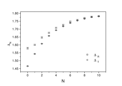
Figure 1: For $\eta=0.1725$ we show $\Delta_{r}$ and $\Delta_{t}$ as the functions of the cycle number $N$. Fitting the curve $\Delta+ce^{-N}$ to the data we obtain $\Delta\approx 1.803$.

Figure 2: Fitting the echoing period $\Delta$ (determined as in Fig. 1) to the analytic prediction $\Delta=a\ln|\eta-\eta_{c}|+const$ we get $\eta_{c}=0.1701$ and the slope $a=-0.389$ which is in very good agreement with the analytic prediction $a=-2/\lambda_{CSS}$ and the linear perturbation result ch $\lambda_{CSS}(\eta_{c})\approx 5.14$.

Let $p^{*}$ be a critical parameter value which separates dispersion from black holes (this value can be found by standard bisection). In agreement with w1 we find that for $\eta>0.17$ the solution corresponding to $p^{*}$ is DSS, in particular for $p$ slightly below $p^{*}$ we observe DSS subcriticality, i.e. the solution approaches the DSS solution and then disperses. Looking at the maximum value of the spatial derivative of the scalar field at the origin as the function of $p$, we find a typical subcritical scaling law (see Fig. 3)

$$\max|\partial_{r}F(t,0)|\sim(p^{*}-p)^{-\gamma_{DSS}}.$$ (5)

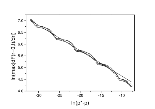
Figure 3: The subcritical scaling (5) for the coupling constant $\eta=0.19$. The slope of the linear fit is approximately equal to $-0.109$. The wiggles, which are imprints of discrete self-similarity, have the period $\approx 4.8$.

For $p>p^{*}$ black holes are formed, however this happens in a rather unusual manner. This is shown in Fig. 4 where the metric function $A$ is seen to develop two minima very close to zero which signals an almost simultaneous formation of a small and a large black hole.

Figure 4: The series of snapshots of the metric function $A(t,r)$ from the evolution of marginally supercritical initial data for the coupling constant $\eta=0.19$. At the last frame one can see the formation of two apparent horizons.

Let us denote their apparent horizon radii by $r_{in}$ and $r_{out}$, respectively. We find that the outer radius exhibits the standard DSS supercritical scaling (see Fig. 5a)

$$r_{outer}\sim(p-p^{*})^{\gamma_{DSS}},$$ (6)

but the inner radius does not seem to scale. The latter fact was already mentioned in w2 . The corresponding graph shows a sea-saw structure, i.e. short straight lines with jump discontinuities at certain values of the parameter $p$ (see Fig. 5b).

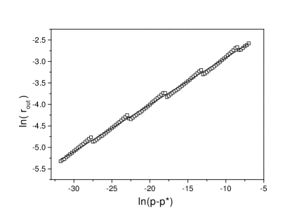
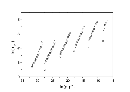
Figure 5: $\eta=0.19$. (a) The locus of the outer apparent horizon is shown to satisfy the power law (6) with the slope $\gamma_{DSS}=0.109$. The wiggles superimposed on the linear fit have the period $4.8$ which agrees with the analytic prediction $\Delta/2\gamma_{DSS}$. (b) The locus of the inner horizon is shown not to scale. The jump discontinuities are periodic with the period $4.8$.

In order to understand this strange behavior we looked in more detail at the evolution of initial data fine-tuned to the location of these jumps. With the help of high resolution numerical methods we found the following remarkable structure: for a given family of initial data there is a sequence of discrete parameter values $p_{1}>p_{2}>p_{3}...>p_{n}$ such that a solution with $p\in(p_{n},p_{n+1})$ approaches to the $CSS_{1}$ solution $n$ times, i.e. the solution comes close to the $CSS_{1}$ solution, turns away and returns $n$ times before leading to black hole formation. Multiple approaches to the $CSS_{1}$ solution were already noticed in w2 where they were called episodic CSS, however the corresponding fine-structure in the parameter space was not seen there. The sequence $\{p_{n}\}$ with $n\leq 5$ is listed in Table 1.

$n$	1	2	3	4	5	$\infty$
$p_{n}$	$0.529001923689295$	$0.528771570563995$	$0.528769577618968$	$0.528769560376615$	$0.528769560227152$	$0.528769560226138$

Table 1: The first five critical parameter values $p_{n}$ for the coupling constant $\eta=0.19$.

Because of numerical limitations we were not able to resolve higher $p_{n}$, however the data shown in Table 1 seem to indicate that the sequence $p_{n}$ converges to $p^{*}$ as $n$ tends to infinity. Actually, we find that the two consecutive parameters $p_{n}$ satisfy the scaling law

$$\frac{p_{n}-p^{*}}{p_{n+1}-p^{*}}\approx\exp\left(\frac{\Delta}{2\gamma_{DSS}}\right).$$ (7)

Now we return to the problem of scaling of the inner radius $r_{in}$. For $p=p_{n}+\varepsilon$, i.e. for $p$ just above one of the $p_{n}$’s we see a clear CSS scaling (see Fig. 6a)

$$r_{in}\sim(p-p_{n})^{\gamma_{CSS}}.$$ (8)

For $p=p_{n}-\varepsilon$ the solution displays a kind of pseudo-dispersion after its last CSS-episode. This pseudo-dispersion manifests itself as follows: after leaving the CSS solution, the maximum of the function $F$ decreases, the inner minimum of $A$ disappears and later a spike develops which leads to the formation of an apparent horizon at $r_{outer}$. In this range of $p$ we see the subcritical CSS scaling (see Fig. 6b)

$$\max|\partial_{r}F(t,0)|\sim(p_{n}-p)^{-\gamma_{CSS}},$$ (9)

however the masses of black holes formed in such evolutions are ”large” and do not scale. We remark that since the solutions on both sides of $p_{n}$ form black holes, the bisection which gives critical parameter values $p_{n}$ has to be performed in a sense ”by hand”.

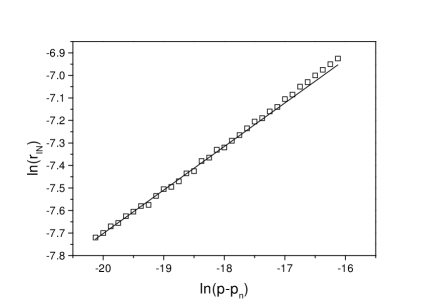
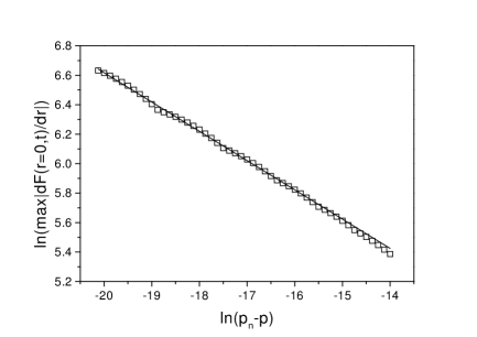
Figure 6: $\eta=0.19$. (a) The supercritical (8) and (b) subcritical (9) scalings around $p_{n}$ for $n=2$ (we get the same picture for each $n$). The slopes of the linear fits are equal to $\pm 0.195$ which agrees with the analytic prediction $\pm 1/\lambda_{CSS}$ where $\lambda_{CSS}(\eta=0.19)=5.1$ was obtained independently from the linear perturbation theory by Lechner ch .

Interpretation of numerical results

The results presented above confirm and extend the findings of Lechner et al. w2 . Probing the bifurcation point $\eta_{c}$ with higher accuracy we improved the evidence that $\Delta$ diverges as $\eta$ tends to the critical value $\eta_{c}=0.17$ from above, which in turn confirms the picture that the DSS cycle merges with the CSS solution at the critical coupling constant $\eta_{c}$. A natural question is: what is the meaning of the series of critical parameter values $p_{n}$ within this picture?

We conjecture that our system shows a so called Shil’nikov bifurcation k . In his classification of loop bifurcations for three dimensional systems, Shil’nikov considered a system with a saddle point together with a homoclinic orbit which bifurcates for some value of a parameter. Assuming that the eigenvalues of the saddle point are real and satisfy the following conditions: $\lambda_{1}>0>\lambda_{2}>\lambda_{3}$ and $\lambda_{1}+\lambda_{2}>0$ (plus some less important technical conditions), Shil’nikov showed that a saddle limit cycle bifurcates and the phase space picture looks qualitatively as in Fig. 7a.

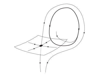
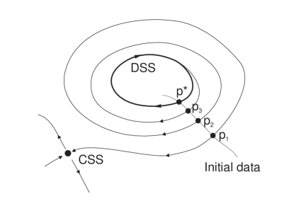
Figure 7: (a) Shil’nikov bifurcation. (b) The conjectured phase space picture.

Of course, our system is infinite dimensional and the Shil’nikov theorem cannot be applied directly. Nevertheless, it is expected that a similar picture to Fig. 7a will be valid for higher dimensional systems as long as only a few largest eigenvalues of the perturbation matter. Recently, Donninger d has studied linear perturbations around the CSS solution and found that for coupling constants around the critical value $\eta_{c}$ the first three largest eigenvalues do in fact satisfy the above stated Shil’nikov conditions. Combining this property with the fact that the bifurcating DSS solution is a saddle limit cycle, we conjecture that the (one-dimensional) unstable manifold of the DSS solution lies on the stable manifold of the neighboring CSS solution. This is sketched in Fig. 7b. More precisely, the DSS unstable manifold winds around the limit cycle (infinitely many times) and eventually runs into the CSS saddle. Suppose that a curve of initial data intersects this spiral manifold at values $p_{n}$, with $\lim p_{n}=p^{*}$, where $p^{*}$ corresponds to the intersection with the limit cycle. Then, the dynamical behavior will have exactly the form we observed above: for $p$ equal to one of the $p_{n}$’s, the solution spirals $n$ times around the limit cycle each time coming closer to the CSS–saddle before hitting it. For $p=p_{n}\pm\varepsilon$, the behavior is similar, except that the solution does not hit the CSS–saddle but escapes along its unstable manifold. This is the reason why one observes the CSS scaling around $p_{n}$ with an exponent related to the unstable eigenvalue of the CSS solution. Note that the scaling law (7) follows immediately from the picture shown in Fig. 7b because during one cycle of evolution the distance from the DSS limit cycle increases by the factor $e^{\lambda_{DSS}\Delta}$ (and $\gamma_{DSS}=1/\lambda_{DSS}$).

References

- (1) S. Husa, Ch. Lechner, M. Pürrer, J. Thornburg, P. C. Aichelburg, Phys.Rev. D62, 104007 (2000).
- (2) P. Bizoń, A. Wasserman, Phys.Rev. D62, 084031 (2000).
- (3) Ch. Lechner, PhD thesis, University of Vienna, 2001; gr-qc/0507009.
- (4) Ch. Lechner, J. Thornburg, S. Husa, P. C. Aichelburg, Phys.Rev. D65, 081501 (2002).
- (5) P. Bizoń, A. Wasserman, Class.Quant.Grav. 19, 3309 (2002).
- (6) P. Bizoń, S. Szybka, A. Wassserman, Phys.Rev. D69, 064014 (2004).
- (7) S. Szybka, Phys.Rev. D69, 084014 (2004).
- (8) C. Gundlach, Phys.Rev. D55, 695 (1997).
- (9) P. Bizoń, T. Chmaj, Z. Tabor, Nonlinearity 13, 1411 (2000).
- (10) P. Bizoń, Commun. Math. Phys. 215, 45 (2000).
- (11) D. H. Bailey et al., ARPREC: An Arbitrary Precision Computation Package, technical report available online at the URL: http://crd.lbl.gov/ dhbailey/dhbpapers/arprec.pdf
- (12) Y. Kuznetsov, Elements of Applied Bifurcation Theory, Springer, New York, 2001.
- (13) R. Donninger, in preparation.