Solving 1-D Special Relativistic Hydrodynamics(SRH) Equations Using Different Numerical Method and Results from Different Test Problems

Abstract

In this paper, we have solved $1D$ special relativistic hydrodynamical equations using different numerical method in computational gas dynamics. The numerical solutions of these equations for smooth wave cases give better solution when we use $Non-TVD$(Total Variable Diminishing) but solution of discontinuity wave produces some oscillation behind the shock. On the other hand, $TVD$ type schemes give good approximation at discontinuity cases. Because $TVD$ schemes completely remove the oscillations, they reduce locally the accuracy of the solution around the extrema.

I INTRODUCTION

The invention of the digital computer and its introduction into the world of science and technology has led to the development, and increased awareness, of the concept of approximation. This concerns the theory of numerical approximation of a set of equations, taken as a mathematical model of a physical system. However, it also concerns the notion of approximation involved in the definition of this mathematical model with respect to the complexity of physical world.We are concerned here with physical systems for which is assumed that the basic equations describing their behavior is known theoretically but for which no analytic solutions exist, and consequently an approximate numerical solution will be sought instead.The approximation is relative to a given time and environment, and these are being extended with the evolution of computer technology.We can state that a mathematical model for the behavior of a astrophysical system, and in particular the system of fluid flows, can only be defined after consideration of the level of the approximation required in order to achieve an acceptable accuracy on a defined set of dependent and independent variables.For instance, evolution of relativistic hydrodynamical system can be considered to depend on conserve and primitive variables.

Actually, physicists propose various levels of description of our physical world, ranging from subatomic or molecular, microscopic or macroscopic up to the astronomical scale. So fluid dynamics is essentially the study of the interactive motion and behavior of a large number of individual elements. From this point of view we understand easily why concept of fluid mechanics can be applied large number of interacting elements, such as astrophysical phenomenon.

The astrophysical problems creates strong shocks region due to strong gravitational field. An accurate description of relativistic cases with strong shocks is needed for study of important problems, such as accreting of compact objects, stellar collapse, and coalescing of compact binaries. At this end, we have started testing different numerical methods to solve the relativistic hydrodynamical equations.

In this paper, first we introduce the special relativistic hydrodynamical(SRH) equation and their components. Second, we give detail discussion about numerical schemes we have used here. Finally, we discuss numerical solution of SRH equation from different numerical schemes when we applied them to the different test problems.

II FORMULATION

The General Relativistic Hydrodynamic (GRH) equations in Refs. Don_Fon and Fon_Mil , written in the standard covariant form, consist of the local conservation laws of the stress-energy tensor $T^{\mu\nu}$ and the matter current density $J^{\mu}$:

$$\bigtriangledown_{\mu}T^{\mu\nu}=0,\;\;\;\;\;\bigtriangledown_{\mu}J^{\mu}=0.$$ (1)

Greek indices run from $0$ to $3$, Latin indices from $1$ to $3$, and units in which the speed of light $c=1$ are used.

Defining the characteristic waves of the general relativistic hydrodynamical equations is not trivial with imperfect fluid stress-energy tensor. We neglect the viscosity and heat conduction effects. This defines the perfect fluid stress-energy tensor. We use this stress-energy tensor to derive the hydrodynamical equations. With this perfect fluid stress-energy tensor, we can solve some problems which are solved by the Newtonian hydrodynamics with viscosity, such as those involving angular momentum transport and shock waves on an accretion disk, etc. Entropy for perfect fluid is conserved along the fluid lines. The stress energy tensor for a perfect fluid is given as

$$T^{\mu\nu}=\rho hu^{\mu}u^{\nu}+Pg^{\mu\nu}.$$ (2)

A perfect fluid is a fluid that moves through spacetime with a 4-velocity $u^{\mu}$ which may vary from event to event. It exhibits a density of mass $\rho$ and isotropic pressure $P$ in the rest frame of each fluid element. $h$ is the specific enthalpy, defined as

$$h=1+\epsilon+\frac{P}{\rho}.$$ (3)

Here $\epsilon$ is the specific internal energy. The equation of state might have the functional form $P=P(\rho,\epsilon)$. The perfect gas equation of state,

$$P=(\Gamma-1)\rho\epsilon,$$ (4)

is such a functional form.

The conservation laws in the form given in Eq.(1) are not suitable for the use in advanced numerical schemes. In order to carry out numerical hydrodynamic evolutions such as those reported in Fon_Mil , and to use high resolution shock capturing schemes, the hydrodynamic equations after the 3+1 split must be written as a hyperbolic system of first order flux conservative equations. We write Eq.(1) in terms of coordinate derivatives, using the coordinates ($x^{0}=t,x^{1},x^{2},x^{3}$). Eq.(1) is projected onto the basis $\{n^{\mu},(\frac{\partial}{\partial x^{i}})^{\mu}\}$, where $n^{\mu}$ is a unit timelike vector normal to a given hypersurface. After a straightforward calculation and neglecting the GR part of equation we get in $1D$ (see ref.Fon_Mil ),

$$\partial_{t}\vec{U}+\partial_{x}\vec{F}^{x}=0,$$ (5)

where $\partial_{t}=\partial/\partial t$ and $\partial_{x}=\partial/\partial x$. This basic step serves to identify the set of unknowns, the vector of conserved quantities $\vec{U}$, and their corresponding fluxes $\vec{F}^{x}(\vec{U})$. With the equations in conservation form, almost every high resolution method devised to solve hyperbolic systems of conservation laws can be extended to GRH.

The evolved state vector $\vec{U}$ consists of the conservative variables $(D,S_{x},\tau)$ which are conserved variables for density, momentum and energy respectively; in terms of the primitive variables $(\rho,v^{x},\epsilon)$, this becomes Fon_Mil

$$\vec{U}=\left(\begin{array}[]{c}D\\ S_{x}\\ \tau\end{array}\right)=\left(\begin{array}[]{c}\sqrt{\gamma}W\rho\\ \sqrt{\gamma}\rho hW^{2}v_{x}\\ \sqrt{\gamma}(\rho hW^{2}-P-W\rho)\end{array}\right).$$ (6)

Here $\gamma$ is the determinant of the 3-metric $\gamma_{xj}$ which is a unit matrix for special relativity, $v_{x}$ is the fluid 3-velocity in $x$ direction, and W is the Lorentz factor,

$$W=\alpha u^{0}=(1-\gamma_{xj}v^{x}v^{j})^{-1/2}.$$ (7)

The flux vectors $\vec{F^{x}}$ are given by Fon_Mil

$$\vec{F}^{x}=\left(\begin{array}[]{c}\alpha v^{x}D\\ \alpha\{v^{x}S_{j}+\sqrt{\gamma}P\delta^{x}_{j}\}\\ \alpha\{v^{x}\tau+\sqrt{\gamma}v^{x}P\}\end{array}\right).$$ (8)

The spatial components of the 4-velocity $u^{x}$ are related to the 3-velocity by the following formula: $u^{x}=Wv^{x}$. $\alpha$, which equals $1$ for special relativistic case, is the lapse function of the spacetime.

The use of HRSC scheme requires the spectral decomposition of the Jacobian matrix of the system, $\partial\vec{F^{x}}/\partial\vec{U}$. The spectral decomposition of the Jacobian matrices of the SRH equations with a general equation of state was reported in Fon_Mil .

We started the solution by considering an equation of state in which the pressure $P$ is a function of $\rho$ and $\epsilon$, $P=P(\rho,\epsilon)$. The relativistic speed of sound in the fluid $C_{s}$ is given by Fon_Mil

$$C_{s}^{2}=\left.\frac{\partial P}{\partial E}\right|_{S}.=\frac{\chi}{h}+\frac{P\kappa}{\rho^{2}h},$$ (9)

where $\chi=\partial P/\partial\rho|_{\epsilon}$, $\kappa=\partial P/\partial\epsilon|_{\rho}$, $S$ is the entropy per particle, and $E=\rho+\rho\epsilon$ is the total rest energy density.

In order to use numerical schemes to solve SRH equation, eigenvalues and left and right eigenvector must be defined for the Jacobian matrix. A complete set of the right and left eigenvectors $[\vec{r}_{i}]$ and corresponding eigenvalues $\lambda_{i}$ along the $x$-direction is given in DONMEZ1 .

In any relativistic hydrodynamics code evolving the conserved quantities $(D,S,\tau)$ in time, the primitive variables $(P,\rho,v)$ have to be computed from the conserved quantities at least once per time step. In our code, this is achieved using relations (4),(3),(6) and (7) to construct the function MM

$$f(P)=(\Gamma-1)\rho_{*}\epsilon_{*}-P,$$ (10)

where Eq. (6) gives

$$\rho_{*}=\frac{D}{\sqrt{\gamma}W_{*}}$$ (11)

and Eqs. (3) and (6) give

$$\epsilon_{*}=\frac{\tau+D(1-W_{*})+\sqrt{\gamma}(1-W_{*}{{}^{2}})P}{DW_{*}}.$$ (12)

Here

$$W_{*}=\frac{1}{\sqrt{1-v^{2}}},$$ (13)

and $v^{2}=\gamma^{jk}v_{j}v_{k}\;=v_{j}v^{j}$.

From Eq.(6), the following relation between $P$, $v$, and the conserved quantities can be derived:

$$v_{j}=\frac{S_{j}}{\tau+\sqrt{\gamma}P+D}.$$ (14)

From Eqs.(13) and (14), we get

$$W_{*}=\frac{1}{\sqrt{1-\frac{S_{j}}{\tau+\sqrt{\gamma}P+D}\gamma^{jk}\frac{S_{k}}{\tau+\sqrt{\gamma}P+D}}}.$$ (15)

Setting $f(P)=0$ in equation (10) gives a nonlinear implicit equation for $P$. It can be solved using a root finding method; in this work, we are using the false-position method NUMREC . The zero of $f(P)$ in the physically allowed domain $P_{min}<P<P_{max}$ determines the pressure, and the monotonicity of $f(P)$ in that domain ensures the uniqueness of the solution MM . The lower bound of the physically allowed domain $P_{min}$, defined by $P_{min}=|S-\tau-D|$, is obtained from (14) by taking into account that (in our units) $|v|\leq 1$, and $P_{max}$ can be taken to have any sufficiently large value. Knowing $P$, Eq.(14) then directly gives $v$, while the remaining state quantities are obtained in a straightforward manner from Eqs.(3), (6), and (7).

III Numerical Schemes and Method

The special relativistic hydrodynamical equations in $1D$ can be written in the form

$$\frac{\partial\vec{U}}{\partial t}+\frac{\partial\vec{F}^{x}}{\partial x}=0,$$ (16)

Discretization of the hydrodynamical equations (16) gives

$$\frac{\partial\vec{U}_{i}}{\partial t}+\frac{(\vec{f^{*}})_{i+1/2}-(\vec{f^{*}})_{i-1/2}}{\bigtriangleup x}=0.$$ (17)

where $(\vec{f^{*}})_{i+1/2}$ is the numerical flux calculated at the interfaces $i\pm 1/2$ of spatial cell $i$.

In here, we will explain the numerical methods we use to solve the hydrodynamical equations. First, we will introduce the flux splitting method in which fluxes are defined depending on the sign of eigenvalues of Jacobian matrix which is defined from SRH equations. Second, we will explain the MUSCL-type schemes, in which the state variables at the interfaces are obtained from an extrapolation between neighboring cell averages.

III.1 Flux Split Method

First, we consider the flux splitting method, in which the flux is decomposed into the part contributing to the eigenfields with positive eigenvalues (fields moving to the right) and the part with negative eigenvalues (fields moving to the left) HIRSCH ; Toro . These fluxes are then discretized with one-sided or upwind differences depending on the sign of the particular eigenvalue. For example, the flux of material moving in the $+x$ direction is differenced with a backward spatial difference.

For the flux split method, one assumes that HIRSCH ; Toro

$$\vec{F}^{x}(\zeta\vec{U})=\zeta\vec{F}^{x}(\vec{U}),$$ (18)

for any constant $\zeta$. This only holds for the fluxes of Eq.(8) if the equation of state has the functional form $P=P(\rho,\epsilon)=\rho f(\epsilon)$, for some function $f(\epsilon)$. Therefore, we use the perfect gas equation of state,

$$P=(\Gamma-1)\rho\epsilon,$$ (19)

where $\Gamma$ is the adiabatic index of the fluid. From the Eq.(18) , the flux vector $\vec{F}^{x}$ can be written

$$\vec{F}^{x}=(\frac{\partial\vec{F}^{x}}{\partial\vec{U}})\vec{U}.$$ (20)

Using the spectral decomposition, one can write the Jacobian matrix $\partial\vec{F}^{x}/\partial\vec{U}$ in the form HIRSCH ; Toro

$$\frac{\partial\vec{F}^{x}}{\partial\vec{U}}=(M^{x})\Lambda^{x}(M^{x})^{-1},$$ (21)

where $M^{x}$ is the matrix whose columns are the right eigenvectors of the system in the x-direction, and $\Lambda^{x}$ is a diagonal matrix constructed from the corresponding eigenvalues which are given in DONMEZ1 .

Next, we split the flux into the part that is moving to the right and the part that is moving to the left. Using Eqs.(20) and (21) this gives HIRSCH ; Toro

$$\vec{F}^{x}=(\vec{F}^{x})^{+}+(\vec{F}^{x})^{-}=\{(M^{x})(\Lambda^{x})^{+}(M^{x})^{-1}\}\vec{U}+$$

$$\{(M^{x})(\Lambda^{x})^{-}(M^{x})^{-1}\}\vec{U},$$ (22)

where $(\Lambda^{x})^{+}=\frac{1}{2}(\Lambda^{x}+|\Lambda^{x}|)$, and $(\Lambda^{x})^{-}=\frac{1}{2}(\Lambda^{x}-|\Lambda^{x}|)$. If we use a first-order upwind flux, we define

$$(\vec{f}^{*}_{i+1/2})=(\vec{F}^{x})^{+}_{i}+(\vec{F}^{x})^{-}_{i+1},$$ (23)

and

$$(\vec{f}^{*}_{i-1/2})=(\vec{F}^{x})^{+}_{i-1}+(\vec{F}^{x})^{-}_{i}.$$ (24)

When these are substituted into Eq.(17), we get

$$\vec{U}^{n+1}_{i}=\vec{U}^{n}_{i}-\frac{\bigtriangleup t}{\bigtriangleup x}[(\vec{F}^{x})^{+}_{i}+(\vec{F}^{x})^{-}_{i+1}-((\vec{F}^{x})^{+}_{i-1}+(\vec{F}^{x})^{-}_{i})]^{n}.$$ (25)

This scheme is first-order accurate in space and time.

Second order accurate flux-splitting method can also be constructed; see DFIM .

III.2 MUSCL-Type Methods

We introduce HRSC(High Resolution Shock Capturing) schemes which use slope limiters to kill spurious oscillations, called MUSCL-type schemes. MUSCL stands for Monotone Upstream-centered Scheme for Conservation Laws. The MUSCL-type scheme allows us to construct higher order methods, fully discrete, semi-discrete and also implicit methods HIRSCH ; Toro . While higher order linear schemes produce spurious oscillations, the MUSCL-type scheme achieves a high order of accuracy by data reconstruction, where the reconstruction is constrained so as to avoid spurious oscillations.

The value of any quantity, $u^{n}_{i}$ represents an integral average in cell $[x_{i-\frac{1}{2}},x_{i+\frac{1}{2}}]$, given by

$$u^{n}_{i}=\frac{1}{\Delta x}\int_{x_{i-\frac{1}{2}}}^{x_{i+\frac{1}{2}}}u(x,t^{n})dx.$$ (26)

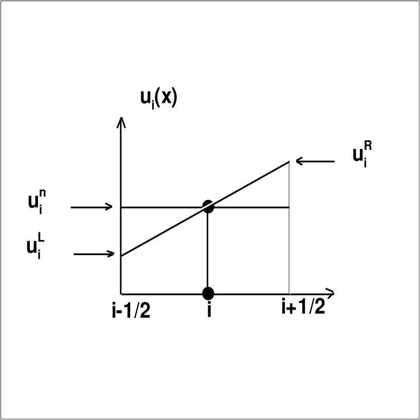
Local reconstruction of $u_{i}(x)$ from Fig.1 is

$$u_{i}(x)=u^{n}_{i}+\frac{(x-x_{i})}{\Delta x}\Delta_{i},\;\;\;\;\;\;\;\;x\;\epsilon\;[0,\Delta x].$$ (27)

where $\frac{\Delta_{i}}{\Delta x}$ is called the slope of $u_{i}(x)$ in cell $i$. Fig.1 shows the specific grid cell $i$. The center of the cell $x_{i}$ in local coordinates is $x=\frac{1}{2}\Delta x$ and $u_{i}(x_{i})=u^{n}_{i}$. From Eq.(27), the values of $u_{i}(x_{i})$ at the left and right edges of the cell play an important role in this reconstruction scheme; they are given by

$$u^{L}_{i}=u_{i}(0)=u_{i}-\frac{1}{2}\Delta_{i}$$

$$u^{R}_{i}=u_{i}(\Delta x)=u_{i}+\frac{1}{2}\Delta_{i}.$$ (28)

These left and right states are called boundary extrapolated values. Note that the integral of $u_{i}(x)$ in cell $i$ is identical to that of $u^{n}_{i}$ and thus the reconstruction process retains flux conservation. This is a second-order accurate scheme, $O(\bigtriangleup x^{2})$.

If we assume the slopes are zero in Eq.(28), the MUSCL scheme becomes the first-order accurate Godunov method.

III.3 Slope Functions

To avoid the appearance of oscillations around discontinuities in MUSCL-type schemes, we will use slope limiters in the reconstruction stage HIRSCH ; Toro .

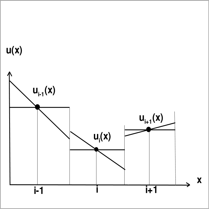
Fig.2 shows the piecewise linear reconstruction process applied to three successive cells. In each cell, we use the slope function defined in Eq.(27) and (28). We will begin by writing the slope function in the form HIRSCH

$$\Delta_{i}=\frac{1}{2}(1+\omega)\Delta u_{i-\frac{1}{2}}+\frac{1}{2}(1-\omega)\Delta u_{i+\frac{1}{2}}$$ (29)

where

$$\Delta u_{i-\frac{1}{2}}\equiv u_{i}^{n}-u_{i-1}^{n},$$

$$\Delta u_{i+\frac{1}{2}}\equiv u_{i+1}^{n}-u_{i}^{n},$$ (30)

and $\omega$ is a free parameter in the interval $[-1,1]$. This produces second-order accurate schemes. For $\omega=0$, $\Delta_{i}$ is a central difference approximation, multiplied by $\Delta x$. For $\omega=-1$, the MUSCL scheme becomes the Lax-Wendroff Method.

In general, schemes based on Eq.(29) still have spurious oscillations at discontinuities. To remove these, we will use limiters that produce schemes which are total variation diminishing, or TVD. A numerical scheme is said to be TVD if

$$TV(U^{n+1})\leq TV(U^{n}),$$ (31)

where the total variation

$$TV(U^{n})=\sum_{i}\mid U_{i+1}-U_{i}\mid.$$ (32)

and $i$ $\rightarrow$ $[-\infty$ , $\infty]$. To apply this rule for any finite number of points on a grid, $U_{i}$ can be set to zero or a constant value outside the grid.

A common TVD limiter is based on the minmod function HIRSCH . The standard minmod slope provides the desired second-order accuracy for smooth solutions, while still satisfying the $TVD$ property. We write this as referring to Fig.2,

$$\Delta_{i}=\rm{minmod}(U_{i}-U_{i-1},U_{i+1}-U_{i}),$$ (33)

where the minmod function of two arguments is defined by:

$$\rm{minmod}(a,b)=\left\{\begin{array}[]{lll}a&\mbox{if $|a|<|b|$ and $ab>0$}\\ b&\mbox{if $|b|<|a|$ and $ab>0$}\\ 0&\mbox{if $ab\leq 0$}.\end{array}\right.$$ (37)

We have also used another TVD slope limiter which may give better solution at discontinuities. This limiter is given by HIRSCH

$$\Delta_{i}=\left\{\begin{array}[]{lll}\rm{max}[0,\rm{min}(\beta\Delta U_{i-\frac{1}{2}},\Delta U_{i+\frac{1}{2}}),\rm{min}(\Delta U_{i-\frac{1}{2}},\beta\Delta U_{i+\frac{1}{2}})],\;\;\;\Delta U_{i+\frac{1}{2}}>0.0\\ \rm{min}[0,\rm{max}(\beta\Delta U_{i-\frac{1}{2}},\Delta U_{i+\frac{1}{2}}),\rm{max}(\Delta U_{i-\frac{1}{2}},\beta\Delta U_{i+\frac{1}{2}})],\;\;\;\Delta U_{i+\frac{1}{2}}<0.0,\par\end{array}\right.$$ (40)

where $1\leq\beta\leq 2$. The value $\beta=1$ reproduces the MINMOD or MINBEE slope limiter as in Eq.(37). $\beta=2$ is called the SUPERBEE flux limiter.

III.4 Marquina Fluxes

Approximate Riemann solver failures and their respective corrections (usually adding a artificial dissipation) have been studied in the literature Quirk . Motivated by the search for a robust and accurate approximate Riemann solver that avoids these common failures, Shu et al ShuOsher have proposed a numerical flux formula for scalar equations. Marquina flux is generalization of flux formula in Ref. ShuOsher . In the scalar case and for characteristic wave speeds which do not change sign at the given numerical interface, Marquina’s flux formula is identical to Roe’s flux Toro . Otherwise, scheme is more viscous, entropy satisfying local Lax-Friedrichs scheme ShuOsher . The combination of Roe and Lax-Friedrichs schemes is carried out in each characteristic field after the local linearization and decoupling of the system of equations. However, contrary to other schemes, the Marquina’s method is not based on any averaged intermediate state.

We use Marquina fluxes with MUSCL left and right states to solve the 1-D relativistic hydro equation. In Marquina’s scheme there are no Riemann solutions involved (exact or approximate) and there are no artificial intermediate states constructed at each cell interface.

To compute the Marquina fluxes we first compute the sided local characteristic variables and fluxes. For the left and right sides, the characteristic variables are

$$w_{l}^{p}=L^{p}(U_{l})\cdot U_{l},\;\;\;\;w_{r}^{p}=L^{p}(U_{r})\cdot U_{r}$$ (41)

and the characteristic fluxes are

$$\Phi_{l}^{p}=L^{p}(U_{l})\cdot F(U_{l}),\;\;\;\;\;\Phi_{r}^{p}=L^{p}(U_{r})\cdot F(U_{r}).$$ (42)

where the number of conservative variables $p=1..5$. $U_{l}$ and $U_{r}$ are conservative variables at the left and right sides, respectively. $L^{p}(U_{l})$ and $L^{p}(U_{r})$ are the left eigenvectors of the Jacobian matrices, $\partial F^{i}/\partial U$.

We define left and right fluxes depending on the velocities of the fluid for each specific grid zone. The prescription given in Ref.DFIM is as follows.

For all conserved variables $p=1,..m$

if $\lambda_{p}(U)$ does not change sign in (if ( $\lambda_{p}(U_{L})$ $\times$ $\lambda_{p}(U_{R})$ $\geq$ 0)), then

     if $\lambda_{p}(U_{l})>0$ then

            $\Phi_{+}^{p}=\Phi_{l}^{p}$

            $\Phi_{-}^{p}=0$

     else

            $\Phi_{+}^{p}=0$

            $\Phi_{-}^{p}=\Phi_{r}^{p}$

     end if

else

            $\alpha_{p}=\max_{U\epsilon\Gamma(U_{l},U_{r})}|\lambda_{p}(U)|$

            $\Phi_{+}^{p}=0.5(\Phi_{l}^{p}+\alpha_{k}w_{l}^{p})$

            $\Phi_{-}^{p}=0.5(\Phi_{r}^{p}+\alpha_{p}w_{r}^{p})$

end if

where $\lambda_{p}$ is an eigenvalue of the Jacobian matrix and,

$$\alpha_{k}=\max\{|\lambda_{p}(U_{l})|,|\lambda_{p}(U_{r})|\}.$$ (43)

The numerical flux that corresponds to the cell interface separating the states $U_{l}$ and $U_{r}$ is then given by Ref.DFIM :

$$F^{M}(U_{l},U_{r})=\sum_{p=1}^{m}(\Phi_{+}^{p}r^{p}(U_{l})+\Phi_{-}^{p}r^{p}(U_{r})).$$ (44)

Marquina’s scheme can be interpreted as a characteristic-based scheme that avoids the use of an averaged intermediate state to perform the transformation to the local characteristic fields.

In carrying out Marquina’s scheme, we have to compute intermediate states and the Jacobian matrix of the states at each cell interface. So we need to know the left and right states, $U_{L}$ and $U_{R}$, at each interface. To construct the second-order scheme, we use the MUSCL left and right states given in Eq.(28).

IV NUMERICAL RESULTS

Results of numerical solution of SRH equation are given. Before doing any further explanation, we need to define boundary conditions. Boundary conditions are set by filling the data in guard cells with appropriate values. In the numerical calculation boundary filling plays an important role in the simulations. The computational grid is extended at both sides of the physical domain to compute the fluxes at interfaces. These extra cells are also called guard cells or ghost zones. There are different types of boundary conditions used in the literature to solve physical problems in an appropriate way. In this paper we have used several types of boundary conditions including periodic, inflow, outflow and analytically prescribed boundary conditions. These boundary conditions have to be provided on each time step for all primitive and conservative variables in the special relativistic hydro code.

Here, we solve three different test problems to compare the results from different numerical schemes.

IV.1 Smooth Test Problems

First, we start testing the code with smooth hydrodynamical solutions using different numerical schemes which are explained in III. Since we are concerned with special relativistic flows, we choose cases with $P\sim\rho$ and $v\sim 1$ in our units ($c=1$). We focus on the case of a varying density profile $\rho=\rho(x,t)$ with constant, uniform pressure $P=P_{0}$ and velocity $v=v_{0}$. When these functions are substituted into Eq. (5), we see that they form a consistent solution for the advection of a density profile at constant velocity $v_{0}$. These tests are performed on the computational domain $0\leq x\leq 1$ with the ideal gas law Eq.(19), with $\Gamma=5/3$.

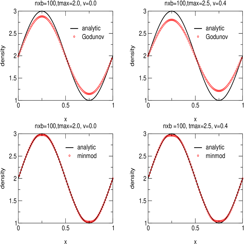
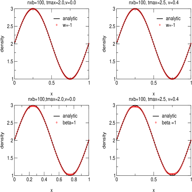
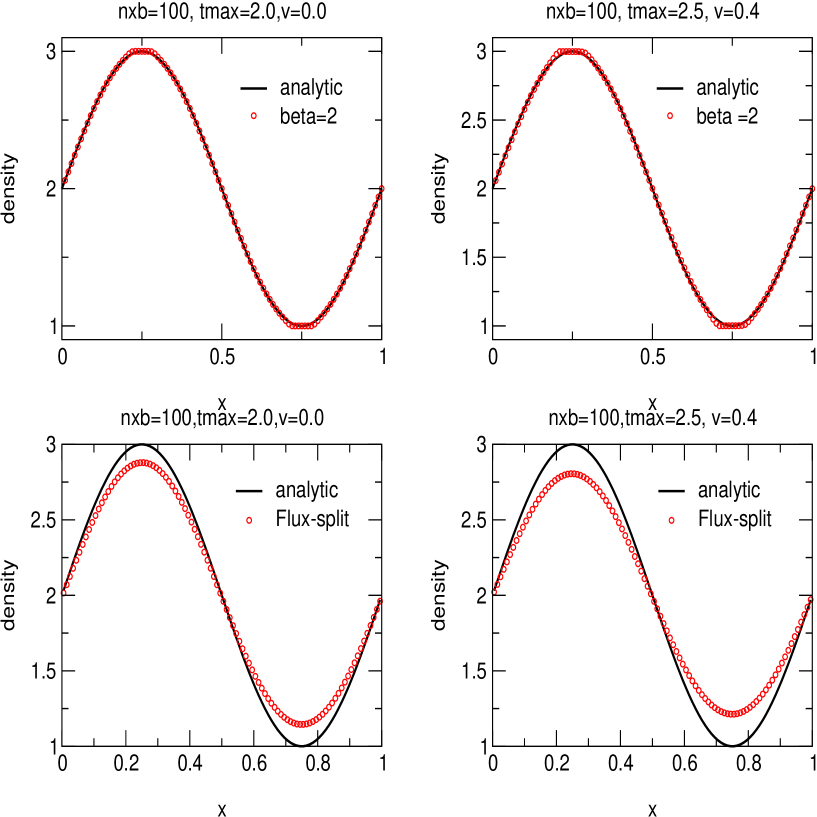
The first test in Table 1 consists of a stationary density pulse.In Table 2 we compute the $L_{1}$ norm errors and convergence rates, $c$, for the different numerical scheme for the standing wave test problem in Table.1. All numerical schemes give a good convergence rate for the standing wave problem, except the minmod schemes. However while $TVD$ schemes completely remove the oscillations, they reduce locally the accuracy of the solution around the extrema. We also compare the numerical solutions of the standing wave, shown in the left-hand panels and labeled with $v=0$, with the analytic solutions using these schemes in Figs. 3, 4 and 5. It is easy to see from these figures that the $TVD$ schemes($minmod$, $\beta=1$ and $\beta=2$) reduce the accuracy of the solution around the extrema. From Fig. 4 with $w=-1$, the Lax-Wendroff scheme gives better solution for the smooth wave.

In Table 3 we compute the $L_{1}$ norm errors and convergence rates,$c$, using the different numerical schemes for the moving wave in Table 1. We got good first-order convergence rates for the flux splitting and Godunov methods. The Lax-Wendroff method gives good convergence rates for second-order method. The convergence rates with $TVD$ schemes are not as good as for Lax-Wendroff, and they are not consistent because of the problems around the extrema. In Figs. 3, 4 and 5, we plot the numerical solutions of the moving wave, shown in the right-hand panels and label with $v=0.4$, with the analytic solutions using different schemes. Again, the $TVD$ schemes reduce the accuracy of the solution around the extrema.

IV.2 Shock Tube Test Problem

Our next code test is the Riemann shock tube HIRSCH ; Toro . In this problem, the fluid is initially in two different thermodynamical states on either side of a membrane. The membrane is then removed. Let us assume that the fluid initially has $\rho_{L}>\rho_{R}$, where the subscripts $L$ and $R$ refer to the left and right sides of the membrane. Then, a rarefaction wave travels to the left, and a shock wave and contact discontinuity travel to the right.The Riemann shock tube is a useful test problem because it has an exact time-dependent solution and tests the ability of the code to evolve both smooth and discontinuous flows. In the case considered here, the velocities are special relativistic and the method of finding the exact solution differs somewhat from the standard non-relativistic shock tube.

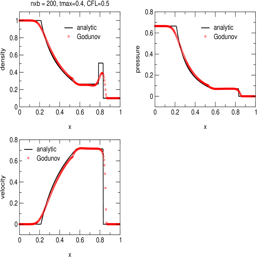
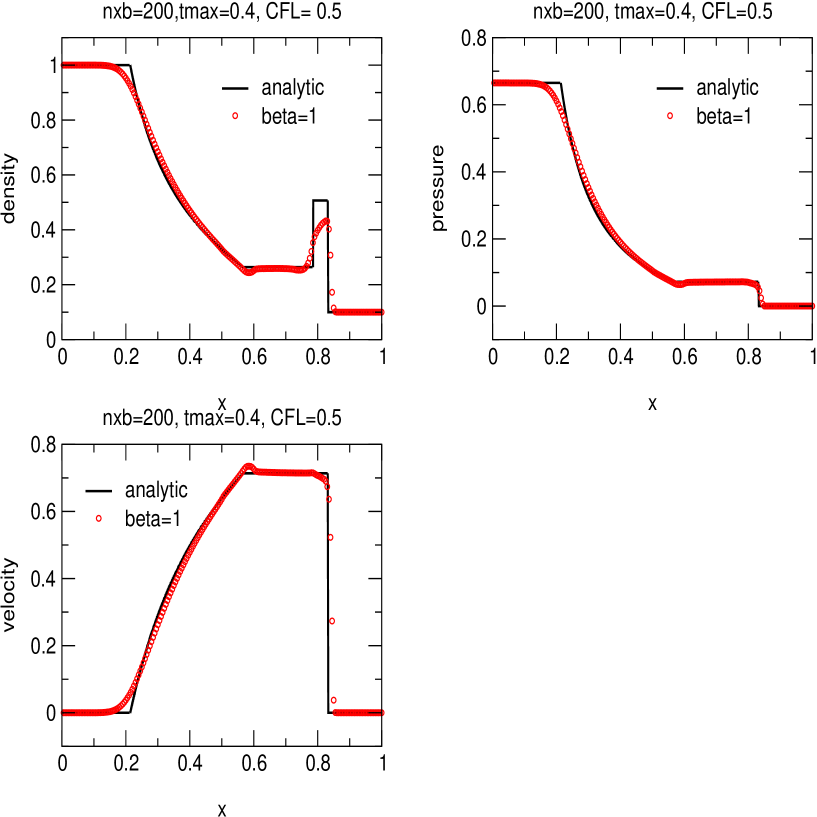
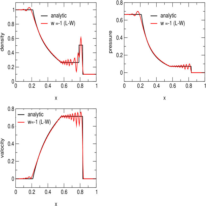
In Table 5 we compute the $L_{1}$ norm errors and convergence rates using the different numerical schemes for the special relativistic shock problem in Table 4. The convergence rates should approach $1$ when we use higher order methods. From the last three columns of Table 5, the first-order flux splitting and Godunov methods give good convergence rates, but not the Lax-Wendroff scheme, which scheme produces spurious oscillation behind the shock. This is seen clearly in Fig.8. The $TVD$ schemes give good convergence rates for the shock tube problem. From Table 5 the $TVD$ schemes give better convergence rates than the flux-splitting and Godunov schemes, because $TVD$ schemes are second-order accurate. Additionally, we plot the analytic and numerical solutions of the shock tube problem for Godunov and $TVD$ with $\beta=1$ in Figs. 6 and 7. We did not compute the convergence rates for $\beta=2$. Because it produce some oscillation and it does not allow to us run the code enough time to compute convergence rates.

V CONCLUSION

Numerical solution of special relativistic hydrodynamical equation in $1D$ using first and second order different numerical methods is explained in this paper. The numerical methods are applied on cases which are stationary and unsteady flow situations. Results from different method are compared to define better method for problems. It is seen from figures and tables that while $TVD$ type schemes gives good approximation for discontinuity solution, the $Non-TVD$ type schemes give better solution for smooth test problems. Because $TVD$ schemes completely remove the oscillations, they reduce locally the accuracy of the solution around the extrema. As a conclusion, $TVD$ type schemes can use to solve astrophysical problems which have strong shock region, especially around the compact objects.

Table 1: Initial data for smooth waves test problems.

Special Relativistic Smooth Wave Test Problems

Test $$\rho$$

1 1.0 0.0

2 1.0 0.4

Table 2: $L_{1}$ norm errors and convergence rates for the standing wave test problem in Table 1. The different first and second-order schemes are used.

L1 norm errors and convergence rates for the standing wave
Type	$npts$	$L_{1}(\rho)$	$L_{1}(p)$	$L_{1}(v)$	$c(\rho)$	$c(p)$	$c(v)$
	100	8.42E-2	1.56E-3	7.84E-4	1.92	1.88	1.84
Flux-splitting	200	4.36E-2	8.29E-4	4.25E-4	1.96	1.94	1.92
$O(\Delta x,\Delta t)$	400	2.22E-2	4.28E-4	2.21E-4	1.98	1.97	1.95
(non-TVD)	800	1.12 E-2	2.16E-4	1.13E-4	1.98	1.99	1.96
	1600	5.64 E-3	1.09E-4	5.77E-5
	100	8.38E-2	1.87E-3	5.67E-4	1.93	1.84	1.82
Godunov	200	4.33E-2	1.01E-3	3.10E-4	1.96	1.92	1.90
$O(\Delta x,\Delta t)$	400	2.20E-2	5.27E-4	1.62E-4	1.98	1.95	1.95
(non-TVD)	800	1.11E-2	2.69E-4	8.33E-5	1.99	1.97	1.97
	1600	5.59E-3	1.36E-4	4.22E-5
w=-1	100	2.87E-3	7.06E-5	2.56E-5	3.99	3.99	4.00
(Lax-Wend.)	200	7.19E-4	1.76E-5	6.39E-6	3.99	3.999	4.00
$O(\Delta x^{2},\Delta t^{2})$	400	1.79E-4	4.41E-6	1.59E-6	3.999	3.999	3.91
(non-TVD)	800	4.49E-5	1.10E-6	4.07E-7
	100	6.55E-3	4.37E-5	2.49E-5	3.67	3.58	3.67
$\beta=1$	200	1.78E-3	1.22E-5	6.79E-6	3.65	3.68	3.68
$O(\Delta x^{2},\Delta t^{2})$	400	4.87E-4	3.32E-6	1.84E-6	3.76	3.79	3.77
(TVD)	800	1.29E-4	8.75E-7	4.89E-7	3.81	3.87	3.84
	1600	3.39E-5	2.25E-7	1.27E-7
	100	4.69 E-3	3.75E-5	1.59E-5	3.53	3.32	2.96
$\beta=2$	200	1.32E-3	1.13E-5	5.37 E-6	3.77	3.53	3.36
$O(\Delta x^{2},\Delta t^{2})$	400	3.51E-4	3.19E-6	1.59E-6	3.88	3.72	3.56
(TVD)	800	9.04 E-5	8.58E-7	4.48E-7	3.94	3.84	3.72
	1600	2.29 E-5	2.23E-7	1.20E-7
	100	6.38E-3	5.47E-4	1.68E-4	3.56	1.80	1.64
minmod	200	1.79E-3	3.03E-4	1.02E-4	3.14	2.95	2.32
$O(\Delta x^{2},\Delta t^{2})$	400	5.69E-4	1.02E-4	4.42E-5	3.22	2.89	3.26
(TVD)	800	1.76E-4	3.55E-5	1.35E-5	2.36	1.32	1.33
	1600	7.45 E-5	2.68E-5	1.01E-5

Table 3: $L_{1}$ norm errors and convergence rates for the moving wave test problem from Table 1. The different first and second order schemes are used.

L1 norm errors and convergence rates for the moving wave
Type	$npts$	$L_{1}(\rho)$	$L_{1}(p)$	$L_{1}(v)$	$c(\rho)$	$c(p)$	$c(v)$
	100	0.129	2.76E-3	8.79E-4	1.89	1.76	1.76
Flux-splitting	200	6.83E-2	1.56E-3	4.97E-4	1.94	1.87	1.87
$O(\Delta x,\Delta t)$	400	3.51E-2	8.33E-4	2.65E-4	1.97	1.93	1.93
(non-TVD)	800	1.78E-2	4.30E-4	1.36E-4	1.98	1.96	1.96
	1600	8.97E-3	2.18E-4	6.95E-5
	100	0.13	2.8E-3	8.8E-4	1.9	1.78	1.78
Godunov	200	6.84E-2	1.58E-3	4.99E-4	1.95	1.89	1.89
$O(\Delta x,\Delta t)$	400	3.54E-2	8.35E-4	2.67E-4	1.98	1.93	1.93
(non-TVD)	800	1.8E-2	4.32E-4	1.38E-4	1.99	1.97	1.97
	1600	8.9E-3	2.2E-4	6.9E-5
w=-1	100	3.94E-3	1.13E-4	3.67 E-5	3.99	3.99	3.99
(Lax-Wend.)	200	9.86E-4	2.83E-5	9.19E-6	4.00	3.99	3.99
$O(\Delta x^{2},\Delta t^{2})$	400	2.46E-4	7.08E-6	2.30E-6	4.00	4.00	3.99
(non-TVD)	800	6.16E-5	1.77E-6	5.75E-7
	100	1.15 E-2	8.65E-5	3.01E-5	3.56	3.95	4.07
$\beta=1$	200	3.22E-3	2.19E-5	7.37E-6	3.67	3.96	4.05
$O(\Delta x^{2},\Delta t^{2})$	400	8.77E-4	5.52E-6	1.81E-6	3.73	3.97	4.01
(TVD)	800	2.34E-4	1.38E-6	4.53E-7	3.81	3.98	4.00
	1600	6.15E-5	3.48E-7	1.13E-7
	100	7.81E-3	8.06E-5	2.94E-5	3.45	3.81	4.43
$\beta=2$	200	2.26E-3	2.11E-5	6.65E-6	3.71	3.91	3.98
$O(\Delta x^{2},\Delta t^{2})$	400	6.09E-4	5.39E-6	1.67E-6	3.85	3.90	3.81
(TVD)	800	1.57E-4	1.38 E-6	4.38E-7	3.92	4.01	3.94
	1600	4.01E-5	3.43E-7	1.11 E-7
	100	1.15E-2	8.67E-5	3.01E-5	3.56	3.86	4.14
minmod	200	3.22E-3	2.24E-5	7.25E-6	3.67	4.05	3.98
$O(\Delta x^{2},\Delta t^{2})$	400	8.77E-4	5.52E-6	1.82E-6	3.73	3.91	4.03
(TVD)	800	2.34E-4	1.41E-6	4.50E-7	3.81	4.04	3.97
	1600	6.15E-5	3.48E-7	1.13E-7

Table 4: Initial data for the special relativistic shock tube test problems

Special Relativistic Test Problem

Test $$\rho_{L}$$

1 10.0 0.0 13.3 1.0 0.0

Table 5: $L_{1}$ norm errors and convergence rates for the shock wave test problem from Table 4. The different first and second order schemes are used.

L1 norm errors and convergence rates for the shock wave
Type	$npts$	$L_{1}(\rho)$	$L_{1}(p)$	$L_{1}(v)$	$r(\rho)$	$r(p)$	$r(v)$
	100	3.72E-1	3.40E-1	4.25E-2	0.58	0.62	0.66
Flux-splitting	200	2.49E-1	2.20E-1	2.68E-2	0.61	0.66	0.72
$O(\Delta x,\Delta t)$	400	1.63E-1	1.38E-1	1.62E-2	0.65	0.698	0.75
(non-TVD)	800	1.03E-1	8.55E-2	9.64E-3	0.70	0.73	0.85
	1600	6.38E-02	5.14E-02	5.33E-03
	100	0.37	0.33	4.23E-2	0.57	0.62	0.66
Godunov	200	0.24	0.22	2.67E-2	0.61	0.66	0.72
$O(\Delta x,\Delta t)$	400	0.16	0.13	1.62E-2	0.65	0.69	0.75
(non-TVD)	800	0.10	8.51E-2	9.62E-3	0.70	0.73	0.85
	1600	6.36E-2	5.12E-2	5.32E-3
w=-1	100	0.22	0.23	1.89E-2	0.29	0.62	0.51
(Lax-Wend.)	200	0.18	0.15	1.32E-2	0.38	0.49	0.31
$O(\Delta x^{2},\Delta t^{2})$	400	0.14	0.11	1.06E-2	2.09E-2	0.22	-0.14
(non-TVD)	800	0.13	9.37E-2	1.17 E-2
	100	0.28	0.25	2.73E-2	0.68	0.66	0.75
$\beta=1$	200	0.17	0.15	1.61E-2	0.80	0.70	0.83
$O(\Delta x^{2},\Delta t^{2})$	400	0.10	9.65E-2	9.08E-3	0.78	0.71	0.79
(TVD)	800	5.85E-2	5.90E-2	5.24E-3	0.76	0.73	0.86
	1600	3.43E-2	3.54E-2	2.88E-3
	100	0.19	0.14	1.95E-2	0.89	0.91	0.87
minmod	200	0.10	7.68E-2	1.06E-2	0.87	0.94	0.89
$O(\Delta x^{2},\Delta t^{2})$	400	5.82E-2	3.99E-2	5.72E-3	0.75	0.93	0.79
(TVD)	800	3.45E-2	2.09E-2	3.31E-3	0.85	0.97	0.99
	1600	1.91E-2	1.06E-2	1.67E-3

Figure 1: Piecewise linear MUSCL reconstruction of a specific grid zone $i$. The boundary extrapolated values are $u^{L}_{i}$ and $u^{R}_{i}$

Figure 2: Piecewise linear MUSCL reconstruction for three successive zones of $i-1$, $i$, $i+1$.

Figure 3: Plot for standing and moving waves using the Godunov method and the MUSCL scheme with the minmod limiter Eq.(37). $npts=100$.

Figure 4: Plot for standing and moving waves using the slopes functions $w=-1$ in Eq.(29)(Lax-Wendroff scheme) and $\beta=1$ in Eq.(40). $npts=100$.

Figure 5: Plot for standing and moving waves using the slope function for$\beta=2$ in Eq.(40) and the flux splitting method. $npts=100$.

Figure 6: The analytic and numerical solutions of the relativistic shock tube problem are plotted. The first-order Godunov scheme is used with resolution   $npts=100$.

Figure 7: The analytic and numerical solutions of the relativistic shock tube problem are plotted. The slope function for $\beta=1$ in Eq.(40) is used with resolution $npts=100$.

Figure 8: The analytic and numerical solutions of the relativistic shock tube problem are plotted. The slope function for $w=-1$ in Eq.(29)(Lax-Wendroff scheme) is used with resolution $npts=100$.