Evolution of Non-linear Fluctuations in Preheating after Inflation

Yasusada Nambu nambu@gravity.phys.nagoya-u.ac.jp    Yohei Araki araki@gravity.phys.nagoya-u.ac.jp Department of Physics, Graduate School of Science, Nagoya University, Chikusa, Nagoya 464-8602, Japan
(November 25, 2005)
Abstract

We investigate the evolution of the non-linear long wavelength fluctuations during preheating after inflation. By using the separate universe approach, the temporal evolution of the power spectrum of the scalar fields and the curvature variable is obtained numerically. We found that the amplitude of the large scale fluctuations is suppressed after non-linear evolution during preheating.

inhomogeneous universe; preheating; back reaction
pacs:
04.25.Nx, 98.80.Hw

I Introduction

Preheating after inflation is a crucial stage in the early universe. Fluctuations of matter fields and gravitational fields are amplified due to the parametric resonance caused by the coherent oscillation of the inflaton fieldTraschenJ:PRD42:1990 ; KofmanL:PRL73:1994 ; KodamaH:PTP96:1996 ; NambuY:1997 ; TaruyaA:1998 . One of the important question on preheating is how the long wavelength metric fluctuation is amplified by the parametric resonance. The linear analysis shows that non-adiabatic modes of long wave fluctuations are amplified and grow during preheating until the non-linear effect by the second order fluctuations becomes dominant. When the non-linear effect cannot be neglected, the backreaction of the fluctuations on the evolution of background quantities becomes dominant and the amplification of long wave modes stops BassetB:PRD62:2000 ; ZibinJP:PRD63:2001 . To obtain complete understanding of the evolution of inhomogeneities during preheating, we have to investigate non-linear evolution of fluctuations .

The separate universe approachWandsD:2000 is an appropriate method to treat the non-linear dynamics of long wavelength fluctuations during preheating. This approach neglects fluctuations of which wavelength is smaller than the Hubble horizon scale. For each spatial point, the basic equation of the separate universe reduces to that of the Friedmann equation for a homogeneous and isotropic flat universe. However, all dynamical variables include non-linear inhomogeneities of which wavelength is larger than the Hubble horizon scale. As the separate universe approach includes all order long wavelength non-linear gravitational fluctuations, we can apply this method to investigate the backreaction effect on evolution of a Friedmann-Robertson-Walker(FRW) universeNambuY:PRD71:2005 .

Tanaka and BassetTanakaT:2003 investigated preheating using the separate universe approach. They found that initial small fluctuations are amplified and evolve to random spatial distribution. In the separate universe, dynamical variables at each spatial point evolve independently. Hence, in the early stage of evolution, fluctuations keep their initial spatial distribution and only the amplitude of fluctuations grows by the parametric resonance. When the amplitude of the massless field grows to be comparable to that of the inflaton field, the non-linear interaction between scalar fields becomes to be dominant and the system enters a chaotic regime. Then, the field variables at each spatial point behave as independent random variables. At this stage, the power spectrum of fluctuations is same as that of random white noise.

In this paper, we concentrate on the evolution of the power spectrum of fluctuations during preheating especially on curvature fluctuation that gives an impact on formation of large scale structure. By performing the numerical simulation of preheating based on the separate universe approach, we aim to understand the feature of evolution of long wavelength non-linear fluctuation during preheating.

The plan of paper is as follows. In Sec. 2, we review the separate universe approach. In Sec. 3, we analytically estimate the evolution of the power spectrum of scalar fields and a curvature variable. We present our numerical results in Sec. 4 and Sec. 5 is devoted to summary and conclusion. We use units in which c==8πG=1𝑐Planck-constant-over-2-pi8𝜋𝐺1c=\hbar=8\pi G=1 throughout the paper.

II Short review of the separate universe approach

The separate universe approachWandsD:2000 is the lowest order spatial gradient expansion (GE)SalopekDS:1992 that is obtained by neglecting all terms containing the second order spatial derivative terms in the Einstein equation. All dynamical variables keep the spatial dependence that represents large scale inhomogeneities whose wavelength is larger than the Hubble horizon scale. In this approach, we assume the following form of the metric :

ds2=N2dt2+e2αd𝒙2,𝑑superscript𝑠2superscript𝑁2𝑑superscript𝑡2superscript𝑒2𝛼𝑑superscript𝒙2ds^{2}=-N^{2}dt^{2}+e^{2\alpha}d\boldsymbol{x}^{2}, (1)

where N𝑁N is a lapse function and α𝛼\alpha is the logarithm of the scale factor of the universe. For the system with two scalar fields ϕi(i=1,2)subscriptitalic-ϕ𝑖𝑖12\phi_{i}~{}(i=1,2), the Einstein equation becomes

3H2=12j(ϕ˙jN)2+V(ϕ1,ϕ2),3superscript𝐻212subscript𝑗superscriptsubscript˙italic-ϕ𝑗𝑁2𝑉subscriptitalic-ϕ1subscriptitalic-ϕ2\displaystyle 3H^{2}=\frac{1}{2}\sum_{j}\left(\frac{\dot{\phi}_{j}}{N}\right)^{2}+V(\phi_{1},\phi_{2}), (2)
iH=12Njϕ˙jiϕj,subscript𝑖𝐻12𝑁subscript𝑗subscript˙italic-ϕ𝑗subscript𝑖subscriptitalic-ϕ𝑗\displaystyle\partial_{i}H=-\frac{1}{2N}\sum_{j}\dot{\phi}_{j}\partial_{i}\phi_{j}, (3)
α˙N=H,H˙N=12j(ϕ˙jN)2,formulae-sequence˙𝛼𝑁𝐻˙𝐻𝑁12subscript𝑗superscriptsubscript˙italic-ϕ𝑗𝑁2\displaystyle\frac{\dot{\alpha}}{N}=H,\quad\frac{\dot{H}}{N}=-\frac{1}{2}\sum_{j}\left(\frac{\dot{\phi}_{j}}{N}\right)^{2}, (4)
1N(ϕ˙jN)˙+3H(ϕ˙jN)+Vϕj=0,1𝑁superscriptsubscript˙italic-ϕ𝑗𝑁˙absent3𝐻subscript˙italic-ϕ𝑗𝑁𝑉subscriptitalic-ϕ𝑗0\displaystyle\frac{1}{N}\left(\frac{\dot{\phi}_{j}}{N}\right)^{\dot{}}+3H\left(\frac{\dot{\phi}_{j}}{N}\right)+\frac{\partial V}{\partial\phi_{j}}=0, (5)

where Eq. (2) is the Hamiltonian constraint, Eq. (3) is the momentum constraint, Eq. (4) and Eq. (5) are evolution equations for the scalar factor and scalar fields.

To understand how the spatial inhomogeneity is included in dynamical variables, it is convenient to use the Hamilton-Jacobi methodSalopekDS:1992 . By introducing the Hubble function H=H(ϕ1,ϕ2)𝐻𝐻subscriptitalic-ϕ1subscriptitalic-ϕ2H=H(\phi_{1},\phi_{2}) that is a function of scalar fields, the above set of equations can be written

3H2=2j(Hϕj)2+V(ϕ1,ϕ2),3superscript𝐻22subscript𝑗superscript𝐻subscriptitalic-ϕ𝑗2𝑉subscriptitalic-ϕ1subscriptitalic-ϕ2\displaystyle 3H^{2}=2\sum_{j}\left(\frac{\partial H}{\partial\phi_{j}}\right)^{2}+V(\phi_{1},\phi_{2}), (6)
iH=jHϕjiϕj,subscript𝑖𝐻subscript𝑗𝐻subscriptitalic-ϕ𝑗subscript𝑖subscriptitalic-ϕ𝑗\displaystyle\partial_{i}H=\sum_{j}\frac{\partial H}{\partial\phi_{j}}\partial_{i}\phi_{j}, (7)
α˙N=H,˙𝛼𝑁𝐻\displaystyle\frac{\dot{\alpha}}{N}=H, (8)
ϕ˙jN=2Hϕj.subscript˙italic-ϕ𝑗𝑁2𝐻subscriptitalic-ϕ𝑗\displaystyle\frac{\dot{\phi}_{j}}{N}=-2\frac{\partial H}{\partial\phi_{j}}. (9)

The solution of the Hamilton-Jacobi equation (6) contains two constants of integration d1(𝒙),d2(𝒙)subscript𝑑1𝒙subscript𝑑2𝒙d_{1}(\boldsymbol{x}),d_{2}(\boldsymbol{x}). If these constants do not have spatial dependence111The constants djsubscript𝑑𝑗d_{j} can have spatial dependence if they satisfy H,ϕ1id1+H,ϕ2id2=0H_{,\phi_{1}}\partial_{i}d_{1}+H_{,\phi_{2}}\partial_{i}d_{2}=0. However, the inhomogeneity caused by disubscript𝑑𝑖d_{i} is related to the decaying mode of perturbations and sub-dominant. Hence we ignore this type of inhomogeneity here., the Hubble function H=H(ϕ1(𝒙),ϕ2(𝒙);d1,d2)𝐻𝐻subscriptitalic-ϕ1𝒙subscriptitalic-ϕ2𝒙subscript𝑑1subscript𝑑2H=H(\phi_{1}(\boldsymbol{x}),\phi_{2}(\boldsymbol{x});d_{1},d_{2}) satisfies the momentum constraint (7). By differentiating H𝐻H with respect to djsubscript𝑑𝑗d_{j}, we have other integration of constants c(𝒙),f(𝒙)𝑐𝒙𝑓𝒙c(\boldsymbol{x}),f(\boldsymbol{x}):

e3αHd1e3c(𝒙),superscript𝑒3𝛼𝐻subscript𝑑1superscript𝑒3𝑐𝒙\displaystyle e^{3\alpha}\frac{\partial H}{\partial d_{1}}\equiv e^{-3c(\boldsymbol{x})}, (10)
e3αHd2e3c(𝒙)f(𝒙).superscript𝑒3𝛼𝐻subscript𝑑2superscript𝑒3𝑐𝒙𝑓𝒙\displaystyle e^{3\alpha}\frac{\partial H}{\partial d_{2}}\equiv e^{-3c(\boldsymbol{x})}f(\boldsymbol{x}). (11)

By solving these equations with respect to ϕjsubscriptitalic-ϕ𝑗\phi_{j}, we can obtain the scale factor dependence of the scalar fields:

ϕ1=ϕ1(α+c(𝒙);f(𝒙),d1,d2),subscriptitalic-ϕ1subscriptitalic-ϕ1𝛼𝑐𝒙𝑓𝒙subscript𝑑1subscript𝑑2\displaystyle\phi_{1}=\phi_{1}(\alpha+c(\boldsymbol{x});f(\boldsymbol{x}),d_{1},d_{2}),
ϕ2=ϕ2(α+c(𝒙);f(𝒙),d1,d2).subscriptitalic-ϕ2subscriptitalic-ϕ2𝛼𝑐𝒙𝑓𝒙subscript𝑑1subscript𝑑2\displaystyle\phi_{2}=\phi_{2}(\alpha+c(\boldsymbol{x});f(\boldsymbol{x}),d_{1},d_{2}). (12)

The gauge invariant variable that reduces to the spatial derivative of the scalar field on the zero curvature gauge is defined byRigopoulosGI:2003

Qi(j)=iϕjϕj,αiα,superscriptsubscript𝑄𝑖𝑗subscript𝑖subscriptitalic-ϕ𝑗subscriptitalic-ϕ𝑗𝛼subscript𝑖𝛼Q_{i}^{(j)}=\partial_{i}\phi_{j}-\phi_{j,\alpha}\partial_{i}\alpha, (13)

and these variables are non-linear generalization of Mukhanov’s gauge invariant variable in the linear perturbation. The scalar field equation (5) in the zero curvature slice iα=0subscript𝑖𝛼0\partial_{i}\alpha=0 is

ϕj,αα+(3+H,αH)ϕj,α+V,ϕjH2=0,\phi_{j,\alpha\alpha}+\left(3+\frac{H_{,\alpha}}{H}\right)\phi_{j,\alpha}+\frac{V_{,\phi_{j}}}{H^{2}}=0,

and by taking the spatial derivative of this equation, it is possible to show that the variable 𝑸i=(Qi(1),Qi(2))subscript𝑸𝑖superscriptsubscript𝑄𝑖1superscriptsubscript𝑄𝑖2\boldsymbol{Q}_{i}=(Q_{i}^{(1)},Q_{i}^{(2)}) satisfies the following evolution equation:

𝑸i,αα+(3+H,αH)𝑸i,α+𝑴𝑸i=0,\displaystyle\boldsymbol{Q}_{i,\alpha\alpha}+\left(3+\frac{H_{,\alpha}}{H}\right)\boldsymbol{Q}_{i,\alpha}+\boldsymbol{M}\boldsymbol{Q}_{i}=0, (14)
;(𝑴)ij=VϕiϕjH2e3αH(e3αHϕi,αϕj,α),α,\displaystyle;(\boldsymbol{M})_{ij}=\frac{V_{\phi_{i}\phi_{j}}}{H^{2}}-\frac{e^{-3\alpha}}{H}\left(e^{3\alpha}H\phi_{i,\alpha}\phi_{j,\alpha}\right)_{,\alpha},

that has the exactly same form as in the linear perturbation case. However, the coefficients of the equations are spatial dependent and this equation describes non-linear evolution of large scale inhomogeneities. The non-linear generalization of the gauge invariant variable in the linear perturbation that reduces to the spatial derivative of the three curvature on the comoving slice is defined by

i=iαNHρ˙totiρtot=iαjϕj,αiϕjjϕj,α2=iαHH˙iH,subscript𝑖subscript𝑖𝛼𝑁𝐻subscript˙𝜌totsubscript𝑖subscript𝜌totsubscript𝑖𝛼subscript𝑗subscriptitalic-ϕ𝑗𝛼subscript𝑖subscriptitalic-ϕ𝑗subscript𝑗superscriptsubscriptitalic-ϕ𝑗𝛼2subscript𝑖𝛼𝐻˙𝐻subscript𝑖𝐻\mathcal{R}_{i}=\partial_{i}\alpha-\frac{NH}{\dot{\rho}_{\text{tot}}}\partial_{i}\rho_{\text{tot}}=\partial_{i}\alpha-\frac{\sum_{j}\phi_{j,\alpha}\partial_{i}\phi_{j}}{\sum_{j}\phi_{j,\alpha}^{2}}=\partial_{i}\alpha-\frac{H}{\dot{H}}\partial_{i}H, (15)

and this quantity can be written using Qisubscript𝑄𝑖Q_{i}:

i=jϕj,αQi(j)jϕj,α2.subscript𝑖subscript𝑗subscriptitalic-ϕ𝑗𝛼superscriptsubscript𝑄𝑖𝑗subscript𝑗superscriptsubscriptitalic-ϕ𝑗𝛼2\mathcal{R}_{i}=-\frac{\sum_{j}\phi_{j,\alpha}Q_{i}^{(j)}}{\sum_{j}\phi_{j,\alpha}^{2}}. (16)

By substituting the solution (12), the gauge invariant quantity 𝑸𝑸\boldsymbol{Q} becomes

𝑸i=(ϕ1,αϕ1,fϕ2,αϕ2,f)(ic(𝒙)if(𝒙))(ϕ1,αϕ2,α)iα,subscript𝑸𝑖matrixsubscriptitalic-ϕ1𝛼subscriptitalic-ϕ1𝑓subscriptitalic-ϕ2𝛼subscriptitalic-ϕ2𝑓matrixsubscript𝑖𝑐𝒙subscript𝑖𝑓𝒙matrixsubscriptitalic-ϕ1𝛼subscriptitalic-ϕ2𝛼subscript𝑖𝛼\boldsymbol{Q}_{i}=\begin{pmatrix}\phi_{1,\alpha}&\phi_{1,f}\\ \phi_{2,\alpha}&\phi_{2,f}\end{pmatrix}\begin{pmatrix}\partial_{i}c(\boldsymbol{x})\\ \partial_{i}f(\boldsymbol{x})\end{pmatrix}-\begin{pmatrix}\phi_{1,\alpha}\\ \phi_{2,\alpha}\end{pmatrix}\partial_{i}\alpha, (17)

and the gauge invariant variable isubscript𝑖\mathcal{R}_{i} becomes

i=iαic+jϕj,αϕj,fjϕj,α2if.subscript𝑖subscript𝑖𝛼subscript𝑖𝑐subscript𝑗subscriptitalic-ϕ𝑗𝛼subscriptitalic-ϕ𝑗𝑓subscript𝑗superscriptsubscriptitalic-ϕ𝑗𝛼2subscript𝑖𝑓\mathcal{R}_{i}=\partial_{i}\alpha-\partial_{i}c+\frac{\sum_{j}\phi_{j,\alpha}\phi_{j,f}}{\sum_{j}\phi_{j,\alpha}^{2}}\partial_{i}f. (18)

If we take the zero curvature slice iα=0subscript𝑖𝛼0\partial_{i}\alpha=0,

i=ic+jϕj,αϕj,fjϕj,α2if.subscript𝑖subscript𝑖𝑐subscript𝑗subscriptitalic-ϕ𝑗𝛼subscriptitalic-ϕ𝑗𝑓subscript𝑗superscriptsubscriptitalic-ϕ𝑗𝛼2subscript𝑖𝑓\mathcal{R}_{i}=-\partial_{i}c+\frac{\sum_{j}\phi_{j,\alpha}\phi_{j,f}}{\sum_{j}\phi_{j,\alpha}^{2}}\partial_{i}f. (19)

From this formula, we can observe that the curvature fluctuation caused by c(𝒙)𝑐𝒙c(\boldsymbol{x}) does not evolve. This mode corresponds to the adiabatic mode in linear perturbation. The curvature fluctuation caused by f(𝒙)𝑓𝒙f(\boldsymbol{x}) corresponds to the non-adiabatic mode and the evolution of the curvature fluctuation is caused by the non-adiabatic mode of scalar fields fluctuations.

III Evolution of inhomogeneities in preheating

In this section, we consider a specific inflationary model with the inflaton field ϕitalic-ϕ\phi and the massless scalar field χ𝜒\chi. The potential is assumed to be

V(ϕ,χ)=λ4ϕ4+g22ϕ2χ2.𝑉italic-ϕ𝜒𝜆4superscriptitalic-ϕ4superscript𝑔22superscriptitalic-ϕ2superscript𝜒2V(\phi,\chi)=\frac{\lambda}{4}\phi^{4}+\frac{g^{2}}{2}\phi^{2}\chi^{2}. (20)

For ϕmplless-than-or-similar-toitalic-ϕsubscript𝑚𝑝𝑙\phi\lesssim m_{pl}, the inflaton field oscillate coherently about ϕ=0italic-ϕ0\phi=0 and the evolution of the χ𝜒\chi field gets the effect of the parametric resonance. For g2/λ=2superscript𝑔2𝜆2g^{2}/\lambda=2 case, the longest wavelength mode k=0𝑘0k=0 is included in a strong resonance band and the fluctuation grows exponentially in time with Floquet index μ0.238𝜇0.238\mu\approx 0.238. Thus, the super-horizon mode is amplified by the parametric resonance. As we are interested in the non-linear evolution of fluctuations, we consider g2/λ=2superscript𝑔2𝜆2g^{2}/\lambda=2 case in which the growth rate for k=0𝑘0k=0 fluctuation is the largest.

III.1 Analytic approximation

In preheating model defined by (20), the time averaged equation of state of the inflaton fields is same as that of radiation and the evolution of the scale factor is given by

eα(tt0+1)1/2,superscript𝑒𝛼superscript𝑡subscript𝑡0112e^{\alpha}\approx\left(\frac{t}{t_{0}}+1\right)^{1/2}, (21)

where we choose α=0𝛼0\alpha=0 at t=0𝑡0t=0. By introducing the conformal time η=𝑑teα𝜂differential-d𝑡superscript𝑒𝛼\eta=\int dte^{-\alpha} and the conformal variables ϕ~=eαϕ,χ~=eαχformulae-sequence~italic-ϕsuperscript𝑒𝛼italic-ϕ~𝜒superscript𝑒𝛼𝜒\tilde{\phi}=e^{\alpha}\phi,\tilde{\chi}=e^{\alpha}\chi, the evolution equations of scalar fields become

ϕ~′′+λϕ~3+g2ϕ~χ~20,superscript~italic-ϕ′′𝜆superscript~italic-ϕ3superscript𝑔2~italic-ϕsuperscript~𝜒20\displaystyle\tilde{\phi}^{\prime\prime}+\lambda\tilde{\phi}^{3}+g^{2}\tilde{\phi}\tilde{\chi}^{2}\approx 0,
χ~′′+g2ϕ~2χ~0,superscript~𝜒′′superscript𝑔2superscript~italic-ϕ2~𝜒0\displaystyle\tilde{\chi}^{\prime\prime}+g^{2}\tilde{\phi}^{2}\tilde{\chi}\approx 0, (22)

where =d/dη{}^{\prime}=d/d\eta. The curvature variable (19) becomes

i14(η0η)2[ϕ~iϕ~+χ~iχ~+O(1η)]subscript𝑖14superscriptsubscript𝜂0𝜂2delimited-[]superscript~italic-ϕsubscript𝑖~italic-ϕsuperscript~𝜒subscript𝑖~𝜒𝑂1𝜂\mathcal{R}_{i}\approx-\frac{1}{4}\left(\frac{\eta_{0}}{\eta}\right)^{2}\left[\tilde{\phi}^{\prime}\partial_{i}\tilde{\phi}+\tilde{\chi}^{\prime}\partial_{i}\tilde{\chi}+O\left(\frac{1}{\eta}\right)\right] (23)

The solution of the separate universe can be written as

ϕ~=ϕ~(η,f(𝒙)),χ~=χ~(η,f(𝒙)),formulae-sequence~italic-ϕ~italic-ϕ𝜂𝑓𝒙~𝜒~𝜒𝜂𝑓𝒙\tilde{\phi}=\tilde{\phi}(\eta,f(\boldsymbol{x})),\quad\tilde{\chi}=\tilde{\chi}(\eta,f(\boldsymbol{x})), (24)

where f(𝒙)𝑓𝒙f(\boldsymbol{x}) is a spatially dependent constant of integration. We obtain perturbative solution by assuming that the amplitude of χ~~𝜒\tilde{\chi} is small:

ϕ~=ϕ~0+ϕ~1+,χ~=χ~1+χ~2+.formulae-sequence~italic-ϕsubscript~italic-ϕ0subscript~italic-ϕ1~𝜒subscript~𝜒1subscript~𝜒2\tilde{\phi}=\tilde{\phi}_{0}+\tilde{\phi}_{1}+\cdots,\qquad\tilde{\chi}=\tilde{\chi}_{1}+\tilde{\chi}_{2}+\cdots. (25)

Then the equations for each order of the perturbation become

ϕ~0′′+λϕ~03=0,superscriptsubscript~italic-ϕ0′′𝜆superscriptsubscript~italic-ϕ030\displaystyle\tilde{\phi}_{0}^{\prime\prime}+\lambda\tilde{\phi}_{0}^{3}=0, (26)
χ~1′′+g2ϕ~02χ~1=0,ϕ~1=0,formulae-sequencesuperscriptsubscript~𝜒1′′superscript𝑔2superscriptsubscript~italic-ϕ02subscript~𝜒10subscript~italic-ϕ10\displaystyle\tilde{\chi}_{1}^{\prime\prime}+g^{2}\tilde{\phi}_{0}^{2}\tilde{\chi}_{1}=0,\quad\tilde{\phi}_{1}=0, (27)
ϕ~2′′+3λϕ~02ϕ~2=g2ϕ~0χ~12,χ~2=0,formulae-sequencesuperscriptsubscript~italic-ϕ2′′3𝜆superscriptsubscript~italic-ϕ02subscript~italic-ϕ2superscript𝑔2subscript~italic-ϕ0superscriptsubscript~𝜒12subscript~𝜒20\displaystyle\tilde{\phi}_{2}^{\prime\prime}+3\lambda\tilde{\phi}_{0}^{2}\tilde{\phi}_{2}=-g^{2}\tilde{\phi}_{0}\tilde{\chi}_{1}^{2},\quad\tilde{\chi}_{2}=0, (28)
χ~3′′+g2ϕ~02χ~3=2g2ϕ~0ϕ~2χ~1.superscriptsubscript~𝜒3′′superscript𝑔2superscriptsubscript~italic-ϕ02subscript~𝜒32superscript𝑔2subscript~italic-ϕ0subscript~italic-ϕ2subscript~𝜒1\displaystyle\tilde{\chi}_{3}^{\prime\prime}+g^{2}\tilde{\phi}_{0}^{2}\tilde{\chi}_{3}=-2g^{2}\tilde{\phi}_{0}\tilde{\phi}_{2}\tilde{\chi}_{1}. (29)

The solution of the background inflaton field ϕ~0subscript~italic-ϕ0\tilde{\phi}_{0} is given by

ϕ~0=ccn(λ1/2cη;1/2)subscript~italic-ϕ0𝑐cnsuperscript𝜆12𝑐𝜂12\tilde{\phi}_{0}=c\,\mathrm{cn}(\lambda^{1/2}c\eta;1/2) (30)

where cncn\mathrm{cn} is the Jacobi elliptic cosine, c𝑐c is the initial value of ϕ~0subscript~italic-ϕ0\tilde{\phi}_{0}. We approximate the elliptic function as followsPBGreeneLKofmanAL:PRD56:1997 :

ϕ~0ccos(τ),ϕ~02c2[F0+F1cos(2τ)],formulae-sequencesubscript~italic-ϕ0𝑐𝜏superscriptsubscript~italic-ϕ02superscript𝑐2delimited-[]subscript𝐹0subscript𝐹12𝜏\displaystyle\tilde{\phi}_{0}\approx c\,\cos(\tau),\quad\tilde{\phi}_{0}^{2}\approx c^{2}\left[F_{0}+F_{1}\cos(2\tau)\right], (31)
τ=2πTλ1/2cη,T=7.416,F0=0.457,F1=0.4973.formulae-sequence𝜏2𝜋𝑇superscript𝜆12𝑐𝜂formulae-sequence𝑇7.416formulae-sequencesubscript𝐹00.457subscript𝐹10.4973\displaystyle\tau=\frac{2\pi}{T}\lambda^{1/2}c\,\eta,\quad T=7.416,~{}F_{0}=0.457,~{}F_{1}=0.4973.

The equation of χ~1subscript~𝜒1\tilde{\chi}_{1} becomes the Mathieu equation and χ~1subscript~𝜒1\tilde{\chi}_{1} grows by the parametric resonance:

χ~1=feμτcosτ,μ0.12g2λformulae-sequencesubscript~𝜒1𝑓superscript𝑒𝜇𝜏𝜏𝜇0.12superscript𝑔2𝜆\tilde{\chi}_{1}=fe^{\mu\tau}\cos\tau,\quad\mu\approx 0.12\frac{g^{2}}{\lambda} (32)

where f𝑓f is a spatially dependent constant of integration which specifies the initial amplitude of χ~~𝜒\tilde{\chi}. The solution up to the third order becomes

ϕ~=[cc1(g2λ)f2ce2μτ]cos(τ)+(sin part + higher frequency part),~italic-ϕdelimited-[]𝑐subscript𝑐1superscript𝑔2𝜆superscript𝑓2𝑐superscript𝑒2𝜇𝜏𝜏(sin part + higher frequency part)\displaystyle\tilde{\phi}=\left[c-c_{1}\left(\frac{g^{2}}{\lambda}\right)\frac{f^{2}}{c}e^{2\mu\tau}\right]\cos(\tau)+\text{($\sin$ part $+$ higher frequency part)}, (33)
χ~=[feμτc2(g2λ)f3c2e3μτ]cos(τ)+(sin part + higher frequency part),~𝜒delimited-[]𝑓superscript𝑒𝜇𝜏subscript𝑐2superscript𝑔2𝜆superscript𝑓3superscript𝑐2superscript𝑒3𝜇𝜏𝜏(sin part + higher frequency part)\displaystyle\tilde{\chi}=\left[fe^{\mu\tau}-c_{2}\left(\frac{g^{2}}{\lambda}\right)\frac{f^{3}}{c^{2}}e^{3\mu\tau}\right]\cos(\tau)+\text{($\sin$ part $+$ higher frequency part)}, (34)
τλ1/2cη,𝜏superscript𝜆12𝑐𝜂\displaystyle\tau\approx\lambda^{1/2}c\eta,

where c1,c2subscript𝑐1subscript𝑐2c_{1},c_{2} are O(1)𝑂1O(1) numerical factors. At the time given by

η1μλ1/2cln(cfλg2),similar-tosubscript𝜂1𝜇superscript𝜆12𝑐𝑐𝑓𝜆superscript𝑔2\eta_{*}\sim\frac{1}{\mu\lambda^{1/2}c}\ln\left(\frac{c}{f}\sqrt{\frac{\lambda}{g^{2}}}\right), (35)

the amplitude of the higher order perturbation terms grow to be comparable to that of the lower order quantities. At this time, fluctuations of χ~~𝜒\tilde{\chi} field changes the evolution of ϕ~~italic-ϕ\tilde{\phi} field through back reaction effect and the exponential growth of fluctuation of χ~~𝜒\tilde{\chi}-field is shut off. After this time, non-linearities become dominant.

As the Eq. (22) is a chaotic system, the behavior of the scalar fields becomes chaotic after this time. The time scale (35) depends on the initial value f(𝒙)𝑓𝒙f(\boldsymbol{x}) of χ~~𝜒\tilde{\chi}-field that is the spatial dependent function. The deviation of the field of neibouring two spatial points grows exponentially for η<η𝜂subscript𝜂\eta<\eta_{*}. After η>η𝜂subscript𝜂\eta>\eta_{*}, as the system is chaotic, the dependence of the initial condition is completely randomized and the spatial distribution of χ~~𝜒\tilde{\chi} becomes that of white noiseTanakaT:2003 .

To evaluate the evolution of the power spectrum of χ~~𝜒\tilde{\chi}, we assume the function f(𝒙)𝑓𝒙f(\boldsymbol{x}) that specifies the initial distribution of χ𝜒\chi obeys the random Gaussian statistics:

f(𝒙)=𝒌f𝒌ei𝒌𝒙,f𝒌1f𝒌2=f02(kkc)nδ𝒌𝟏𝒌𝟐f𝒌=f𝒌,formulae-sequence𝑓𝒙subscript𝒌subscript𝑓𝒌superscript𝑒𝑖𝒌𝒙formulae-sequencedelimited-⟨⟩subscript𝑓subscript𝒌1subscriptsuperscript𝑓subscript𝒌2superscriptsubscript𝑓02superscript𝑘subscript𝑘𝑐𝑛subscript𝛿subscript𝒌1subscript𝒌2subscript𝑓𝒌subscriptsuperscript𝑓𝒌f(\boldsymbol{x})=\sum_{\boldsymbol{k}}f_{\boldsymbol{k}}\,e^{i\boldsymbol{k}\cdot\boldsymbol{x}},\quad\langle f_{\boldsymbol{k}_{1}}f^{*}_{\boldsymbol{k}_{2}}\rangle=f_{0}^{2}\left(\frac{k}{k_{c}}\right)^{n}\delta_{\boldsymbol{k_{1}}\boldsymbol{k_{2}}}\quad f_{\boldsymbol{k}}=f^{*}_{-\boldsymbol{k}}, (36)

where kcsubscript𝑘𝑐k_{c} is a cut off of wave number and f0subscript𝑓0f_{0} defines the amplitude of the power at k=kc𝑘subscript𝑘𝑐k=k_{c}. The actual initial power spectrum for the χ𝜒\chi-field expected to be produced during inflation in this model is investigated by Zibin et al.ZibinJP:PRD63:2001 Owing to their result, the initial spectrum of χ𝜒\chi-field for large scales is given by n=3𝑛3n=-3 and scale invariant. In this paper, as we are interested in feature of non-linear evolutions of fluctuations, we does not fix the value of power index of χ𝜒\chi-field. The power spectrum of χ~~𝜒\tilde{\chi} field is given by

𝒫χ~=(k/kc)3|χ~𝒌|2C1e2μτ(kkc)n+3+C2g2λc2e4μτ(kkc)2n+6,subscript𝒫~𝜒superscript𝑘subscript𝑘𝑐3delimited-⟨⟩superscriptsubscript~𝜒𝒌2subscript𝐶1superscript𝑒2𝜇𝜏superscript𝑘subscript𝑘𝑐𝑛3subscript𝐶2superscript𝑔2𝜆superscript𝑐2superscript𝑒4𝜇𝜏superscript𝑘subscript𝑘𝑐2𝑛6\mathcal{P}_{\tilde{\chi}}=(k/k_{c})^{3}\langle|\tilde{\chi}_{\boldsymbol{k}}|^{2}\rangle\approx C_{1}e^{2\mu\tau}\left(\frac{k}{k_{c}}\right)^{n+3}+C_{2}\frac{g^{2}}{\lambda c^{2}}e^{4\mu\tau}\left(\frac{k}{k_{c}}\right)^{2n+6}, (37)

where C1,C2subscript𝐶1subscript𝐶2C_{1},C_{2} are O(1)𝑂1O(1) numerical factors. At ηηsimilar-to𝜂subscript𝜂\eta\sim\eta_{*}, the amplitude of the fluctuation with the wave number

(kkc)(λc2g2)1n+3exp(2μλ1/2cηn+3).similar-tosubscript𝑘subscript𝑘𝑐superscript𝜆superscript𝑐2superscript𝑔21𝑛32𝜇superscript𝜆12𝑐subscript𝜂𝑛3\left(\frac{k_{*}}{k_{c}}\right)\sim\left(\frac{\lambda c^{2}}{g^{2}}\right)^{\frac{1}{n+3}}\exp\left(-\frac{2\mu\lambda^{1/2}c\eta_{*}}{n+3}\right). (38)

becomes O(1)𝑂1O(1) and non-linear. Once the fluctuation with the wave number ksubscript𝑘k_{*} becomes non-linear, as the system is chaotic, the coherence beyond the scale 1/k1subscript𝑘1/k_{*} is lost and the fluctuation with the wave number k<k𝑘subscript𝑘k<k_{*} is randomized and behaves as white noise. Thus, the power spectrum for k<k𝑘subscript𝑘k<k_{*} becomes that of white noise k3proportional-toabsentsuperscript𝑘3\propto k^{3}. The evolution of the shape of the power spectrum depends on the value of the initial power index n𝑛n.

For n<3𝑛3n<-3, as the power of smaller k𝑘k mode is larger, the smaller k𝑘k mode (large scale) goes to be non-linear first. At ηηsimilar-to𝜂subscript𝜂\eta\sim\eta_{*}, fluctuation with the wave number k<k𝑘subscript𝑘k<k_{*} reaches non-linear and the power spectrum becomes 𝒫χ~k3similar-tosubscript𝒫~𝜒superscript𝑘3\mathcal{P}_{\tilde{\chi}}\sim k^{3}. At this time, fluctuation with the wave number k>k𝑘subscript𝑘k>k_{*} stays linear and the spectrum keeps its initial shape 𝒫χ~kn+3similar-tosubscript𝒫~𝜒superscript𝑘𝑛3\mathcal{P}_{\tilde{\chi}}\sim k^{n+3}. Thus, the shape of the power spectrum at ηηsimilar-to𝜂subscript𝜂\eta\sim\eta_{*} is given by

𝒫χ~(k){k3(k<k)kn+3(k>k)similar-tosubscript𝒫~𝜒𝑘casessuperscript𝑘3𝑘subscript𝑘superscript𝑘𝑛3𝑘subscript𝑘\mathcal{P}_{\tilde{\chi}}(k)\sim\begin{cases}k^{3}\quad&(k<k_{*})\\ k^{n+3}\quad&(k>k_{*})\end{cases} (39)

For n>3𝑛3n>-3, large k𝑘k modes (small scale) goes to non-linear first. Once the smallest scale of the system becomes non-linear at ηηsimilar-to𝜂subscript𝜂\eta\sim\eta_{*}, the coherence of larger scale fluctuation is lost and the spectrum for all wave number changes to be that of the white noise:

𝒫χ~(k)k3(k<k)similar-tosubscript𝒫~𝜒𝑘superscript𝑘3𝑘subscript𝑘\mathcal{P}_{\tilde{\chi}}(k)\sim k^{3}\quad(k<k_{*}) (40)

The power spectrum of the curvature variable isubscript𝑖\mathcal{R}_{i} is given by

𝒫i(k)C3e4μττ4(kkc)n+5+C4g2λμ2c2e6μττ4(kkc)2n+8subscript𝒫subscript𝑖𝑘subscript𝐶3superscript𝑒4𝜇𝜏superscript𝜏4superscript𝑘subscript𝑘𝑐𝑛5subscript𝐶4superscript𝑔2𝜆superscript𝜇2superscript𝑐2superscript𝑒6𝜇𝜏superscript𝜏4superscript𝑘subscript𝑘𝑐2𝑛8\mathcal{P}_{\mathcal{R}_{i}}(k)\approx C_{3}\frac{e^{4\mu\tau}}{\tau^{4}}\left(\frac{k}{k_{c}}\right)^{n+5}+C_{4}\frac{g^{2}}{\lambda\mu^{2}c^{2}}\frac{e^{6\mu\tau}}{\tau^{4}}\left(\frac{k}{k_{c}}\right)^{2n+8} (41)

where C3,C4subscript𝐶3subscript𝐶4C_{3},C_{4} are O(1)𝑂1O(1) numerical factors. At ηηsimilar-to𝜂subscript𝜂\eta\sim\eta_{*}, the power spectrum for n<3𝑛3n<-3 is

𝒫i(k){k3(k<k)kn+5(k>k)similar-tosubscript𝒫subscript𝑖𝑘casessuperscript𝑘3𝑘subscript𝑘superscript𝑘𝑛5𝑘subscript𝑘\mathcal{P}_{\mathcal{R}_{i}}(k)\sim\begin{cases}k^{3}\quad&(k<k_{*})\\ k^{n+5}\quad&(k>k_{*})\end{cases} (42)

For n>3𝑛3n>-3, the spectrum at ηηsimilar-to𝜂subscript𝜂\eta\sim\eta_{*} is

𝒫i(k)k3(k<k)similar-tosubscript𝒫subscript𝑖𝑘superscript𝑘3𝑘subscript𝑘\mathcal{P}_{\mathcal{R}_{i}}(k)\sim k^{3}\quad(k<k_{*}) (43)

We summarize the result of the analytic estimation of the power spectrum in TABLE 1.

n<3𝑛3n<-3
η<η𝜂subscript𝜂\eta<\eta_{*} η>η𝜂subscript𝜂\eta>\eta_{*}
𝒫χsubscript𝒫𝜒\mathcal{P}_{\chi} kn+3superscript𝑘𝑛3k^{n+3} k3(k<k),kn+3(k>k)superscript𝑘3𝑘subscript𝑘superscript𝑘𝑛3𝑘subscript𝑘k^{3}~{}(k<k_{*}),\quad k^{n+3}~{}(k>k_{*})
𝒫isubscript𝒫subscript𝑖\mathcal{P}_{\mathcal{R}_{i}} kn+5superscript𝑘𝑛5k^{n+5} k3(k<k),kn+5(k>k)superscript𝑘3𝑘subscript𝑘superscript𝑘𝑛5𝑘subscript𝑘k^{3}~{}(k<k_{*}),\quad k^{n+5}~{}(k>k_{*})
n>3𝑛3n>-3
η<η𝜂subscript𝜂\eta<\eta_{*} η>η𝜂subscript𝜂\eta>\eta_{*}
𝒫χsubscript𝒫𝜒\mathcal{P}_{\chi} kn+3superscript𝑘𝑛3k^{n+3} k3superscript𝑘3k^{3}
𝒫isubscript𝒫subscript𝑖\mathcal{P}_{\mathcal{R}_{i}} kn+5superscript𝑘𝑛5k^{n+5} k3superscript𝑘3k^{3}
Table 1: Power spectrums of χ𝜒\chi and isubscript𝑖\mathcal{R}_{i} for 333-dimensional space. The initial χ𝜒\chi is scale invariant for n=3𝑛3n=-3.

To compare the numerical calculation performed in the following sections, we present the estimation of the power spectrum for 1-dimensional case (TABLE 2). The initial spectrums are assumed to be

𝒫χkn+1,𝒫ikn+3.formulae-sequenceproportional-tosubscript𝒫𝜒superscript𝑘𝑛1proportional-tosubscript𝒫subscript𝑖superscript𝑘𝑛3\mathcal{P}_{\chi}\propto k^{n+1},\quad\mathcal{P}_{\mathcal{R}_{i}}\propto k^{n+3}. (44)
n<1𝑛1n<-1
η<η𝜂subscript𝜂\eta<\eta_{*} η>η𝜂subscript𝜂\eta>\eta_{*}
𝒫χsubscript𝒫𝜒\mathcal{P}_{\chi} kn+1superscript𝑘𝑛1k^{n+1} k(k<k),kn+1(k>k)𝑘𝑘subscript𝑘superscript𝑘𝑛1𝑘subscript𝑘k~{}(k<k_{*}),\quad k^{n+1}~{}(k>k_{*})
𝒫isubscript𝒫subscript𝑖\mathcal{P}_{\mathcal{R}_{i}} kn+3superscript𝑘𝑛3k^{n+3} k(k<k),kn+3(k>k)𝑘𝑘subscript𝑘superscript𝑘𝑛3𝑘subscript𝑘k~{}(k<k_{*}),\quad k^{n+3}~{}(k>k_{*})
n>1𝑛1n>-1
η<η𝜂subscript𝜂\eta<\eta_{*} η>η𝜂subscript𝜂\eta>\eta_{*}
𝒫χsubscript𝒫𝜒\mathcal{P}_{\chi} kn+1superscript𝑘𝑛1k^{n+1} k𝑘k
𝒫isubscript𝒫subscript𝑖\mathcal{P}_{\mathcal{R}_{i}} kn+3superscript𝑘𝑛3k^{n+3} k𝑘k
Table 2: Power spectrums of χ𝜒\chi and isubscript𝑖\mathcal{R}_{i} for 111-dimensional space. The initial χ𝜒\chi is scale invariant for n=1𝑛1n=-1.

III.2 Numerical simulation of preheating

To confirm the analytic estimation of the evolution of the power spectrums, we perform 1-dimensional lattice simulation of the separate universe.

By introducing the momentum variables Pϕ=ϕ˙/N,Pχ=χ˙/Nformulae-sequencesubscript𝑃italic-ϕ˙italic-ϕ𝑁subscript𝑃𝜒˙𝜒𝑁P_{\phi}=\dot{\phi}/N,P_{\chi}=\dot{\chi}/N, our basic equations of the separate universe are

3H2=12(Pϕ2+Pχ2)+V(ϕ,χ),3superscript𝐻212superscriptsubscript𝑃italic-ϕ2superscriptsubscript𝑃𝜒2𝑉italic-ϕ𝜒\displaystyle 3H^{2}=\frac{1}{2}(P_{\phi}^{2}+P_{\chi}^{2})+V(\phi,\chi), (45)
iH=12(Pϕiϕ+Pχiχ),subscript𝑖𝐻12subscript𝑃italic-ϕsubscript𝑖italic-ϕsubscript𝑃𝜒subscript𝑖𝜒\displaystyle\partial_{i}H=-\frac{1}{2}(P_{\phi}\partial_{i}\phi+P_{\chi}\partial_{i}\chi), (46)
α˙N=H,H˙N=12(Pϕ2+Pχ2),formulae-sequence˙𝛼𝑁𝐻˙𝐻𝑁12superscriptsubscript𝑃italic-ϕ2superscriptsubscript𝑃𝜒2\displaystyle\frac{\dot{\alpha}}{N}=H,\quad\frac{\dot{H}}{N}=-\frac{1}{2}(P_{\phi}^{2}+P_{\chi}^{2}), (47)
ϕ˙N=Pϕ,P˙ϕN=3HPϕVϕ,formulae-sequence˙italic-ϕ𝑁subscript𝑃italic-ϕsubscript˙𝑃italic-ϕ𝑁3𝐻subscript𝑃italic-ϕ𝑉italic-ϕ\displaystyle\frac{\dot{\phi}}{N}=P_{\phi},\quad\frac{\dot{P}_{\phi}}{N}=-3HP_{\phi}-\frac{\partial V}{\partial\phi}, (48)
χ˙N=Pχ,P˙χN=3HPχVχ.formulae-sequence˙𝜒𝑁subscript𝑃𝜒subscript˙𝑃𝜒𝑁3𝐻subscript𝑃𝜒𝑉𝜒\displaystyle\frac{\dot{\chi}}{N}=P_{\chi},\quad\frac{\dot{P}_{\chi}}{N}=-3HP_{\chi}-\frac{\partial V}{\partial\chi}. (49)

As the initial condition, we must prepare variables (H,Pϕ,Pχ,ϕ,χ)𝐻subscript𝑃italic-ϕsubscript𝑃𝜒italic-ϕ𝜒(H,P_{\phi},P_{\chi},\phi,\chi) that satisfy the Hamiltonian constraint (45) and the momentum constraint (46). We adopt the following form of the initial condition :

H=h0,Pχ=0,χ=χ0(x),ϕ=ϕ0,formulae-sequence𝐻subscript0formulae-sequencesubscript𝑃𝜒0formulae-sequence𝜒subscript𝜒0𝑥italic-ϕsubscriptitalic-ϕ0H=h_{0},\quad P_{\chi}=0,\quad\chi=\chi_{0}({x}),\quad\phi=\phi_{0}, (50)

where h0subscript0h_{0} and ϕ0subscriptitalic-ϕ0\phi_{0} are spatially homogeneous constants and χ0(x)subscript𝜒0𝑥\chi_{0}({x}) is the spatially dependent function that specifies the initial inhomogeneity of the χ𝜒\chi-field. We prepare χ0(x)subscript𝜒0𝑥\chi_{0}(x) as a random Gaussian field:

χ0(x)=k>0A^kcos(kx+θ^k)subscript𝜒0𝑥subscript𝑘0subscript^𝐴𝑘𝑘𝑥subscript^𝜃𝑘\chi_{0}(x)=\sum_{k>0}\hat{A}_{k}\cos(kx+\hat{\theta}_{k}) (51)

where θ^ksubscript^𝜃𝑘\hat{\theta}_{k} is a uniform random number in [0,2π]02𝜋[0,2\pi] and A^ksubscript^𝐴𝑘\hat{A}_{k} is a random number whose probability distribution is given by the Rayleigh distribution

P(Ak)Akexp(Ak2χ0(k/kc)n)proportional-to𝑃subscript𝐴𝑘subscript𝐴𝑘superscriptsubscript𝐴𝑘2subscript𝜒0superscript𝑘subscript𝑘𝑐𝑛P(A_{k})\propto A_{k}\exp\left(-\frac{A_{k}^{2}}{\chi_{0}(k/k_{c})^{n}}\right) (52)

where n𝑛n is the power index of the field. We choose kc=πNgrid/Lsubscript𝑘𝑐𝜋subscript𝑁grid𝐿k_{c}=\pi N_{\text{grid}}/L where L𝐿L is the size of the calculating region and Ngridsubscript𝑁gridN_{\text{grid}} is number of grids. This value is the smallest wave number that corresponds to the size of the system. The value of the momentum of the inflaton field is determined by the Hamiltonian constraint (45):

Pϕ=[6h022V(ϕ0,χ0(x))]1/2.subscript𝑃italic-ϕsuperscriptdelimited-[]6superscriptsubscript022𝑉subscriptitalic-ϕ0subscript𝜒0𝑥12P_{\phi}=\left[6h_{0}^{2}-2V(\phi_{0},\chi_{0}({x}))\right]^{1/2}. (53)

Once the initial values that satisfy the Hamiltonian constraint and the momentum constraint, these constraints are preserved during temporal evolution.

We then must specify the time slicing condition to evolve the system. The simplest one is the synchronous slicing N=1𝑁1N=1. In this slice, the evolution equations become

α˙=H,H˙=12(Pϕ2+Pχ2),formulae-sequence˙𝛼𝐻˙𝐻12superscriptsubscript𝑃italic-ϕ2superscriptsubscript𝑃𝜒2\displaystyle\dot{\alpha}=H,\quad\dot{H}=-\frac{1}{2}(P_{\phi}^{2}+P_{\chi}^{2}), (54)
ϕ˙=Pϕ,P˙ϕ=3HPϕλϕ3g2ϕχ2,formulae-sequence˙italic-ϕsubscript𝑃italic-ϕsubscript˙𝑃italic-ϕ3𝐻subscript𝑃italic-ϕ𝜆superscriptitalic-ϕ3superscript𝑔2italic-ϕsuperscript𝜒2\displaystyle\dot{\phi}=P_{\phi},\quad\dot{P}_{\phi}=-3HP_{\phi}-\lambda\phi^{3}-g^{2}\phi\chi^{2}, (55)
χ˙=Pχ,P˙χ=3HPχg2ϕ2χ.formulae-sequence˙𝜒subscript𝑃𝜒subscript˙𝑃𝜒3𝐻subscript𝑃𝜒superscript𝑔2superscriptitalic-ϕ2𝜒\displaystyle\dot{\chi}=P_{\chi},\quad\dot{P}_{\chi}=-3HP_{\chi}-g^{2}\phi^{2}\chi. (56)

One of the other choice is the comoving slice. In this slice, the Hubble parameter H𝐻H is treated as a time parameter (t=H𝑡𝐻t=H) and the evolution equations become

1NαH=H,1N=12(Pϕ2+Pχ2),formulae-sequence1𝑁𝛼𝐻𝐻1𝑁12superscriptsubscript𝑃italic-ϕ2superscriptsubscript𝑃𝜒2\displaystyle\frac{1}{N}\frac{\partial\alpha}{\partial H}=H,\quad\frac{1}{N}=-\frac{1}{2}(P_{\phi}^{2}+P_{\chi}^{2}), (57)
1NϕH=Pϕ,1NPϕH=3HPϕλϕ3g2ϕχ2,formulae-sequence1𝑁italic-ϕ𝐻subscript𝑃italic-ϕ1𝑁subscript𝑃italic-ϕ𝐻3𝐻subscript𝑃italic-ϕ𝜆superscriptitalic-ϕ3superscript𝑔2italic-ϕsuperscript𝜒2\displaystyle\frac{1}{N}\frac{\partial\phi}{\partial H}=P_{\phi},\quad\frac{1}{N}\frac{\partial P_{\phi}}{\partial H}=-3HP_{\phi}-\lambda\phi^{3}-g^{2}\phi\chi^{2}, (58)
1NχH=Pχ,1NPχH=3HPχg2ϕ2χ.formulae-sequence1𝑁𝜒𝐻subscript𝑃𝜒1𝑁subscript𝑃𝜒𝐻3𝐻subscript𝑃𝜒superscript𝑔2superscriptitalic-ϕ2𝜒\displaystyle\frac{1}{N}\frac{\partial\chi}{\partial H}=P_{\chi},\quad\frac{1}{N}\frac{\partial P_{\chi}}{\partial H}=-3HP_{\chi}-g^{2}\phi^{2}\chi. (59)

The second equation of Eq. (57) determines the lapse function N𝑁N. In our numerical calculation, we adopt the synchronous slicing N=1𝑁1N=1 for the sake of the technical simplicity. We also assume that the α𝛼\alpha is homogeneous at initial time and we have only non-adiabatic mode of curvature fluctuation initially.

We solve Eqs (54)-(56) using the 4th order Runge-Kutta method.

IV numerical results

The spatial grid number used is 214=16384superscript214163842^{14}=16384 and the power spectrums are obtained by taking ensemble average of 100 different calculations for different initial distribution of χ𝜒\chi field with the same spectral index. We used the parameter λ=0.1,g2=0.2,ϕ0=0.5,χ0=105,h0=0.03formulae-sequence𝜆0.1formulae-sequencesuperscript𝑔20.2formulae-sequencesubscriptitalic-ϕ00.5formulae-sequencesubscript𝜒0superscript105subscript00.03\lambda=0.1,g^{2}=0.2,\phi_{0}=0.5,\chi_{0}=10^{-5},h_{0}=0.03.

IV.1 flat space case

We first performed the numerical calculation of the scalar fields system in flat space (22) to investigate the evolution of non-linear fluctuation without gravitational effect. We obtained the evolution of the power spectrum of χ~~𝜒\tilde{\chi}-field numerically.

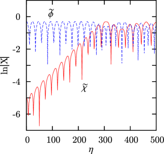
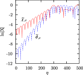
The local evolution of the inflaton field and the massless field is shown in Fig. 1. The spatial derivative of the fields is calculated for two different initial values χ~0=0.5×105,105subscript~𝜒00.5superscript105superscript105\tilde{\chi}_{0}=0.5\times 10^{-5},10^{-5}.

Refer to caption
Refer to caption
Figure 1: The left panel shows the evolution of the scalar fields at a specific spatial point. The right panel shows the evolution of the spatial derivative ϕ~,x\tilde{\phi}_{,x} and χ~,x\tilde{\chi}_{,x}.

In this calculation, the time scale given by Eq. (35) at which non-linear effect becomes significant, is

η280.similar-tosubscript𝜂280\eta_{*}\sim 280.

For ηηless-than-or-similar-to𝜂subscript𝜂\eta\lesssim\eta_{*}, the amplitude of χ~~𝜒\tilde{\chi} field grows exponentially in time by the parametric amplification while the amplitude of ϕ~~italic-ϕ\tilde{\phi} field stays constant. In accordance with this behavior, the spatial derivative of χ~~𝜒\tilde{\chi} and ϕ~~italic-ϕ\tilde{\phi} grows exponentially in time. The growth rate of ϕ~,x\tilde{\phi}_{,x} is greater than that of χ~,x\tilde{\chi}_{,x} and at ηηsimilar-to𝜂subscript𝜂\eta\sim\eta_{*}, ϕ~,xχ~,x\tilde{\phi}_{,x}\sim\tilde{\chi}_{,x}. After ηηsimilar-to𝜂subscript𝜂\eta\sim\eta_{*}, the system enters non-linear regime and the grow of χ~,ϕ~,x,χ~,x\tilde{\chi},\tilde{\phi}_{,x},\tilde{\chi}_{,x} stops.

We next investigate the evolution of the power spectrum of χ~~𝜒\tilde{\chi} for different initial power indices.

n=3𝑛3n=-3 case

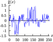
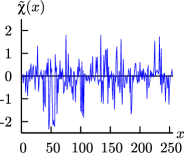
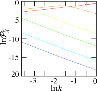
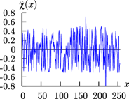
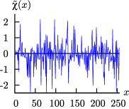
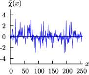
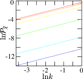
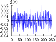
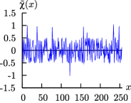
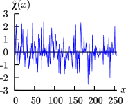
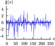
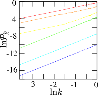
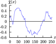
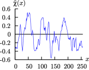
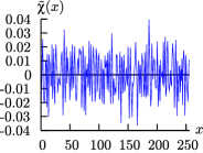
Fig. 2 is the evolution of spatial distribution of χ~~𝜒\tilde{\chi}. Initial smooth distribution evolves to random one. Up to ηsubscript𝜂\eta_{*}, the amplitude of χ~~𝜒\tilde{\chi} grows keeping its initial distribution. After ηsubscript𝜂\eta_{*}, χ~~𝜒\tilde{\chi} begins chaotic behavior and the correlation of the spatial pattern is lost. Fig. 3 shows the evolution of power spectrum of χ~~𝜒\tilde{\chi}. In this case, larger scale has greater power of fluctuation. At η=η280𝜂subscript𝜂similar-to280\eta=\eta_{*}\sim 280, the fluctuation of the largest scale reaches non-linear and the characteristic scale ksubscript𝑘k_{*} appears in the form of the power spectrum. For k<k𝑘subscript𝑘k<k_{*}, the initial power index 33-3 changes to be 111 that corresponds to white noise. The spectrum for k>k𝑘subscript𝑘k>k_{*} keeps its initial slope and a bend at k=k𝑘subscript𝑘k=k_{*} appears in the power spectrum. As time goes on, the value of ksubscript𝑘k_{*} becomes larger and the spectrum for k<kc𝑘subscript𝑘𝑐k<k_{c} becomes that of white noise 𝒫kproportional-to𝒫𝑘\mathcal{P}\propto k when ksubscript𝑘k_{*} reaches kcsubscript𝑘𝑐k_{c}. Thus, although the large scale fluctuation reaches O(1)𝑂1O(1) and becomes non-linear temporally, its amplitude decreases to be smaller than unity when the fluctuation with smaller scale reaches non-linear.
Refer to caption
Refer to caption
Refer to caption
Refer to caption
Figure 2: Evolution of the spatial distribution of χ~~𝜒\tilde{\chi} field for the initial power index n+1=2𝑛12n+1=-2. From the left to the right panel, η=0,280,310,400𝜂0280310400\eta=0,280,310,400.
Refer to caption
Figure 3: Evolution of the power spectrum of χ~~𝜒\tilde{\chi} field for the initial power index n+1=2𝑛12n+1=-2. The spectrums at time η=0(blue),100(cyan),200(green),300(yellow),400(orange),500(red)𝜂0(blue)100(cyan)200(green)300(yellow)400(orange)500(red)\eta=0\text{(blue)},100\text{(cyan)},200\text{(green)},300\text{(yellow)},400\text{(orange)},500\text{(red)} are shown.

n=1𝑛1n=-1 case

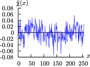
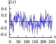
In this case, the initial power spectrum of the χ~~𝜒\tilde{\chi} field is scale invariant. Fig. 4 shows the evolution of spatial distribution of χ~~𝜒\tilde{\chi} and Fig. 5 shows the evolution of power spectrum of χ~~𝜒\tilde{\chi}. Before ηsubscript𝜂\eta_{*}, the spectrum evolves keeping its initial power index 00 and all scales goes to non-linear simultaneously at η=η𝜂subscript𝜂\eta=\eta_{*}. Then the power index changes to be 111 for all k𝑘k. As the same as n=3𝑛3n=-3 case, the power of the large scale fluctuation is suppressed after the amplitude of the fluctuation reaches non-linear.
Refer to caption
Refer to caption
Refer to caption
Refer to caption
Figure 4: Evolution of the spatial distribution of χ~~𝜒\tilde{\chi} field for the initial power index n+1=0𝑛10n+1=0. From the left to the right panel, η=0,260,300,400𝜂0260300400\eta=0,260,300,400.
Refer to caption
Figure 5: Evolution of the power spectrum of χ~~𝜒\tilde{\chi} field for the initial power index n+1=0𝑛10n+1=0 at η=0(blue),100(cyan),200(green),300(yellow),400(orange),500(red)𝜂0(blue)100(cyan)200(green)300(yellow)400(orange)500(red)\eta=0\text{(blue)},100\text{(cyan)},200\text{(green)},300\text{(yellow)},400\text{(orange)},500\text{(red)}.

n=0𝑛0n=0 case

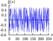
In this case, the initial spectrum is same as that of white noise and the small scale reaches non-linear first. Fig. 6 shows the evolution of spatial distribution of χ~~𝜒\tilde{\chi} and Fig. 7 shows the evolution of power spectrum of χ~~𝜒\tilde{\chi}. As the initial spectrum is same as that of white noise, the power index does not change during whole evolution.
Refer to caption
Refer to caption
Refer to caption
Refer to caption
Figure 6: Evolution of the spatial distribution of χ~~𝜒\tilde{\chi} field for the initial power index n+1=1𝑛11n+1=1. From the left to the right panel, η=0,100,200,300𝜂0100200300\eta=0,100,200,300.
Refer to caption
Figure 7: The power spectrum of χ~~𝜒\tilde{\chi} field for the initial power index n+1=1𝑛11n+1=1 at η=0(blue),100(cyan),200(green),300(yellow),400(orange),500(red)𝜂0(blue)100(cyan)200(green)300(yellow)400(orange)500(red)\eta=0\text{(blue)},100\text{(cyan)},200\text{(green)},300\text{(yellow)},400\text{(orange)},500\text{(red)}.

n=1𝑛1n=1 case

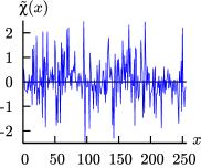
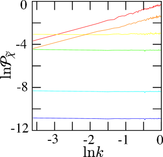
In this case, the initial power index is larger than that of the white noise. Fig. 8 shows the evolution of spatial distribution of χ~~𝜒\tilde{\chi} and Fig. 9 shows the evolution of power spectrum of χ~~𝜒\tilde{\chi}. After the small scale reaches non-linear, the initial power index 222 reduced to be 111.

Refer to caption
Refer to caption
Refer to caption
Refer to caption
Figure 8: Evolution of the spatial distribution of χ~~𝜒\tilde{\chi} field for the initial power index n+1=2𝑛12n+1=2. From the left to the right panel, η=0,260,300,400𝜂0260300400\eta=0,260,300,400.
Refer to caption
Figure 9: Evolution of the power spectrum of χ~~𝜒\tilde{\chi} field for the initial power index n+1=2𝑛12n+1=2 at η=0(blue),100(cyan),200(green),300(yellow),400(orange),500(red)𝜂0(blue)100(cyan)200(green)300(yellow)400(orange)500(red)\eta=0\text{(blue)},100\text{(cyan)},200\text{(green)},300\text{(yellow)},400\text{(orange)},500\text{(red)}.

IV.2 Cosmological case

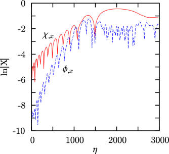
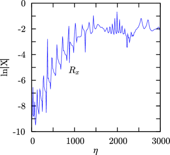
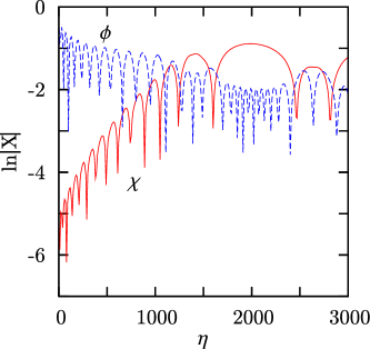
We next solve Eqs (54), (58), (56), and investigate the evolution of the long wavelength metric fluctuations. The behavior of variables at a specific spatial point is shown in Fig. 10 and Fig. 11.
Refer to caption
Refer to caption
Figure 10: In the left panel, evolution of scalar fields at a specific spatial point is shown. In the right panel, evolution of the spatial derivative of the scalar fields is shown.
Refer to caption
Figure 11: Evolution of the curvature variable isubscript𝑖\mathcal{R}_{i} at a specific spatial point.

The characteristic cosmic time when the system becomes non-liner is given by

t=12H0+H02η21460.subscript𝑡12subscript𝐻0subscript𝐻02superscriptsubscript𝜂2similar-to1460t_{*}=-\frac{1}{2H_{0}}+\frac{H_{0}}{2}\eta_{*}^{2}\sim 1460.

Until this time, χ,x\chi_{,x} grows exponentially in conformal time and ϕ,x\phi_{,x} also grows exponentially in accord with the growth of χ,x\chi_{,x} with larger growth rate than that of χ,x\chi_{,x}. We must take care that the amplitude of the spatial derivative of the scalar fields does not reach unity at ttsimilar-to𝑡subscript𝑡t\sim t_{*}. This is due to the suppression of the cosmic expansion but the non-linear regime begins at tsubscript𝑡t_{*}. At ttsimilar-to𝑡subscript𝑡t\sim t_{*}, χ,xϕ,x\chi_{,x}\sim\phi_{,x} and the back reaction of χ𝜒\chi on the evolution of ϕitalic-ϕ\phi begins to be significant and the growth of the fluctuation caused by the parametric resonance stops. The evolution of metric variables H,α,i𝐻𝛼subscript𝑖H,\alpha,\mathcal{R}_{i} is same as the evolution of χ,x\chi_{,x} and they grow until ttsimilar-to𝑡subscript𝑡t\sim t_{*} when the back reaction cannot be neglected.

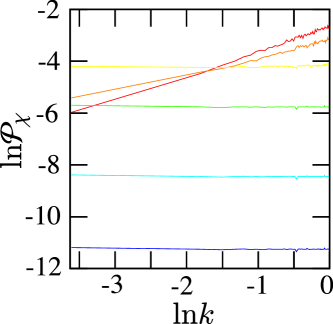
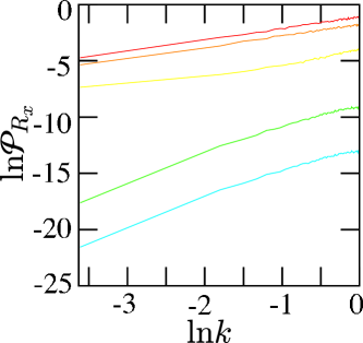
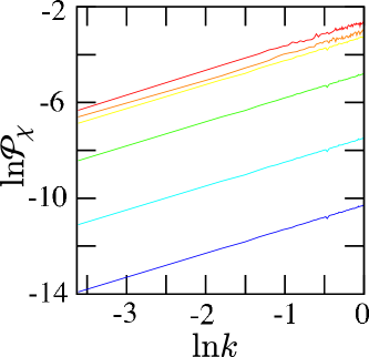
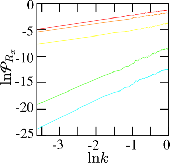
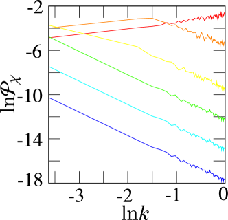
Evolution of the power spectrums of χ𝜒\chi and isubscript𝑖\mathcal{R}_{i} depends on the initial power index of the χ𝜒\chi field. The evolution of the power spectrum of χ𝜒\chi is qualitatively same as the flat space case. For n=3𝑛3n=-3 (Fig. 12), until ttsimilar-to𝑡subscript𝑡t\sim t_{*}, the spectrum of isubscript𝑖\mathcal{R}_{i} keeps its initial flat shape k0superscript𝑘0k^{0}. At ttsimilar-to𝑡subscript𝑡t\sim t_{*}, the large scale fluctuation of χ𝜒\chi field goes to be non-linear and the bend of the spectrum of isubscript𝑖\mathcal{R}_{i} at k=k𝑘subscript𝑘k=k_{*} appears. The spectrum of isubscript𝑖\mathcal{R}_{i} becomes k𝑘k for k<k𝑘subscript𝑘k<k_{*}. The amplitude of the curvature variable isubscript𝑖\mathcal{R}_{i} stays less than unity during whole evolution.
Refer to caption
Refer to caption
Figure 12: Evolution of the power spectrums for the initial power index n+1=2𝑛12n+1=-2 case. The left panel is 𝒫χsubscript𝒫𝜒\mathcal{P}_{\chi} and the right panel is 𝒫isubscript𝒫subscript𝑖\mathcal{P}_{\mathcal{R}_{i}}. Time is t=0𝑡0t=0(blue), 400(cyan), 800(green), 1200(yellow), 1600(orange), 2000(red).

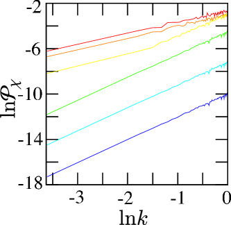
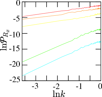
For n1𝑛1n\geq-1 (Fig. 13, Fig. 14, Fig. 15), until ttsimilar-to𝑡subscript𝑡t\sim t_{*}, the spectrum of isubscript𝑖\mathcal{R}_{i} keeps its initial shape kn+3superscript𝑘𝑛3k^{n+3}. At ttsimilar-to𝑡subscript𝑡t\sim t_{*}, the small scale fluctuation of χ𝜒\chi field goes to be non-linear and after this time, the spectrum of isubscript𝑖\mathcal{R}_{i} becomes k𝑘k for all wave number. The amplitude of the curvature variable isubscript𝑖\mathcal{R}_{i} stays less than unity during whole evolution.
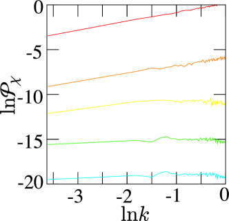
Refer to caption
Refer to caption
Figure 13: Evolution of the power spectrums for the initial power index n+1=0𝑛10n+1=0 case. The left panel is 𝒫χsubscript𝒫𝜒\mathcal{P}_{\chi} and the right panel is 𝒫isubscript𝒫subscript𝑖\mathcal{P}_{\mathcal{R}_{i}}. Time is t=0(blue),400(cyan),800(green),1200(yellow),1600(orange),2000(red)𝑡0(blue)400(cyan)800(green)1200(yellow)1600(orange)2000(red)t=0\text{(blue)},400\text{(cyan)},800\text{(green)},1200\text{(yellow)},1600\text{(orange)},2000\text{(red)}.
Refer to caption
Refer to caption
Figure 14: Evolution of the power spectrums for the initial power index n+1=1𝑛11n+1=1 case. The left panel is 𝒫χsubscript𝒫𝜒\mathcal{P}_{\chi} and the right panel is 𝒫isubscript𝒫subscript𝑖\mathcal{P}_{\mathcal{R}_{i}}. Time is t=0(blue),400(cyan),800(green),1200(yellow),1600(orange),2000(red)𝑡0(blue)400(cyan)800(green)1200(yellow)1600(orange)2000(red)t=0\text{(blue)},400\text{(cyan)},800\text{(green)},1200\text{(yellow)},1600\text{(orange)},2000\text{(red)}.
Refer to caption
Refer to caption
Figure 15: Evolution of the power spectrums for the initial power index n+1=2𝑛12n+1=2 case. The left panel is 𝒫χsubscript𝒫𝜒\mathcal{P}_{\chi} and the right panel is 𝒫isubscript𝒫subscript𝑖\mathcal{P}_{\mathcal{R}_{i}}. Time is t=0(blue),400(cyan),800(green),1200(yellow),1600(orange),2000(red)𝑡0(blue)400(cyan)800(green)1200(yellow)1600(orange)2000(red)t=0\text{(blue)},400\text{(cyan)},800\text{(green)},1200\text{(yellow)},1600\text{(orange)},2000\text{(red)}.

V Summary and discussion

In this paper, we investigated the evolution of long wavelength fluctuations during preheating after inflation. By using the separate universe approach, we obtained the evolution of the power spectrum of long wavelength fluctuations numerically. During the linear stage of the evolution, the fluctuation of the massless field grows exponentially in time by the parametric amplification, but the power spectrum keeps its initial shape. When the fluctuation of the massless field becomes non-linear, the amplification of fluctuations stops by the back reaction effect of massless field on the inflaton field. After this time, the system enters the chaotic non-linear stage and the shape of the spectrum changes. For large scale mode, the amplitude of the fluctuation is suppressed because the statistical nature of the large scale mode becomes that of white noise after the non-linear evolution. The evolution of the curvature variable that has an important role in the cosmological scenario is qualitatively same as the evolution of the scalar field fluctuations. Hence we do not expect the significant effect of the parametric amplification during preheating on the evolution of the large scale fluctuations of metric variables. On the other hand, for small scale fluctuations, the power grows for larger k𝑘k and this leads to the possibility of the formation of the non-linear structures such as primordial black holesSuyamaT:PRD71:2005 .

Acknowledgements.
This work was supported in part by a Grant-In-Aid for Scientific Research of the Ministry of Education, Science, Sports, and Culture of Japan (11640270).

References

  • (1) Traschen J and Brandenberger R H 1990 Particle production during out-of-equilibrium phase transitions Phys. Rev. D 42 2491–2504
  • (2) Kofman L, Linde A and Starobinsky A 1994 Reheating after Inflation Phys. Rev. Lett. 73 3195–3198
  • (3) Kodama H and Hamazaki T 1996 Evolution of Cosmological Perturbations in a Stage Dominated by an Oscillatory Scalar Field Prog. Theor. Phys. 96 949–970
  • (4) Nambu Y and Taruya A 1997 Evolution of Cosmological Perturbation in Reheating Phase of the Universe Prog. Theor. Phys. 97 83–89
  • (5) Taruya A and Nambu Y 1998 Cosmological Perturbation with two scalar fields in Reheating after Inflation Phys. Lett. B428 37–43
  • (6) Basset B and Viniegra F 2000 Massless metric preheating Phys. Rev. D 62 043507
  • (7) Zibin J P, Brandenberger R H and Scott D 2001 Backreaction and the parametric resonance of cosmological fluctuations Phys. Rev. D 63 043511
  • (8) Wands D, Malik K A, Lyth D H and Liddle A R 2000 New approach to the evolution of cosmological perturbations on large scales Phys. Rev. D 62 043527
  • (9) Nambu Y 2005 The separate universe and the backreaction of long wavelength fluctuations Phys. Rev. D 71 084016:1–5
  • (10) Tanaka T and Basset B 2003 Application of the Separate Universe Approach to Preheating astro-ph/0302544
  • (11) Salopek D S and Stewart J M 1992 Hamilton-Jacobi theory for General Relativity with Matter Fields Class. Quantum Grav. 9 1943–1967
  • (12) Rigopoulos G I and Shellard E P S 2003 Separate Universe Approach and the Evolution of Nonlinear Superhorizon Cosmological Perturbations Phys. Rev. D 68 123518:1–8
  • (13) Greene P B, Kofman L, Linde A and Starobinsky A A 1997 Structure of resonance in preheating after inflation Phys. Rev. D 56 6175–6192
  • (14) Suyama T, Tanaka T, Basset B and Kudoh H 2005 Are black holes overproduced during preheating? Phys. Rev. D 71 063507