Quasinormal Modes of Black Holes and Dissipative Open Systems

Abstract

After explaining the physical origin of the quasinormal modes of perturbations in the background geometry of a black hole, I critically review the recent proposal for the quantization of the black-hole area based on the real part of quasinormal modes. As instantons due to the barriers of black-hole potentials lie at the root of a discrete set of complex quasinormal modes frequencies, it is likely that the physics of quasinormal modes can be learned from quantum theory. I propose a connection of a system of quasinormal modes of black holes with a dissipative open system, in particular, the Feshbach-Tikochinsky oscillator. This argument is supported in part by the fact that these two systems have the same group structure $SU(1,1)$ and the same group representation of Hamiltonians; thereby, their quantum states exhibit the same behavior.
Keywords: Quasinormal modes, Black Hole, Dissipative open system

I Introduction

In linear perturbation theory, a perturbed black hole emits waves that are outgoing to spatial infinity and the event horizon. The wave function with this boundary condition is called a quasinormal mode of the black hole and has a complex frequency, whose imaginary part leads to a decaying behavior. There are several motivations to study quasinormal modes of black holes. The original motivation is that quasinormal modes carry carry information of black hole, such as mass, charge, and angular momentum, and may be observed by a gravitational wave detector vishveshwara . Another motivation comes from a recent argument that the real part of the quasinormal mode frequency may play a role in explaining the quantization of the black-hole area hod ; kunstatter ; horowitz . The quantization of the black-hole area, which is believed to be closely related with the microscopic origin of black-hole entropy, is also explained in loop quantum gravity dreyer . Ideas have been suggested to understand the origin of quasinormal modes and various methods have been developed to find quasinormal modes (for review and references, see Refs. kokkotas ; natario ). Quite recently, I have suggested that the quantum theory of quasinormal modes might be related with a dissipative open system and possibly with black-hole thermodynamics kim0 ; kim1 .

The purpose of this paper is not to develop any new method for finding analytically quasinormal modes, but to exploit the physical interpretation of quasinormal modes of black holes. In particular, I shall provide some supporting arguments for my recent proposal on the connection of quasinormal modes with a dissipative open system, the Feshbach-Tikochinsky (FT) oscillator, and possibly with the thermodynamics of black holes in a semiclassical approach. There are some open questions about quasinormal modes and thermodynamics. First, is there any connection between a system of quasinormal modes and a dissipative open system? Second, is there any connection between quasinormal modes and black-hole thermodynamics? It is known that perturbations of a system may provide some information of the system, and, in some cases, may carry all information. Then, what black-hole physics can we learn from quasinormal modes?

II What are Quasinormal Modes of Black Holes?

Let us consider perturbations in a Schwarzchild black hole with mass $M$. The equation for perturbations is given by

$$\frac{\partial^{2}}{\partial t^{2}}\Psi-\frac{\partial^{2}}{\partial r_{*}^{2}}+V(r_{*})\Psi=0,$$ (1)

where $r_{*}=r+2M\ln(r/2M-1)$ is the tortoise coordinate. In the mode decomposition

$$\Psi_{\omega lm}(t,r,\theta,\phi)=e^{i\omega t}\psi_{(\omega l)}(r_{*})Y_{lm}(\theta,\phi),$$ (2)

the perturbation equation is separated as

$$-\frac{\partial^{2}}{\partial r_{*}^{2}}\psi_{(\omega l)}+V_{(l)}(r_{*})\psi_{(\omega l)}=\omega^{2}\psi_{(\omega l)}.$$ (3)

The potential of the Schwarzschild black hole is given by

$$V_{(l)}=\Bigl{(}1-\frac{2M}{r}\Bigr{)}\Bigl{(}\frac{l(l+1)}{r^{2}}+\frac{2\sigma M}{r^{3}}\Bigr{)},$$ (4)

where scalar $(l\geq 0)$, electromagnetic $(l\geq 1)$ and gravitational $(l\geq 2)$ perturbations have $\sigma=1,0,-3$, respectively. For instance, Fig. 1 shows the first few black hole potentials for the scalar perturbation. There is a potential barrier for each $l$.

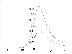
Figure 1: The black hole potentials for scalar perturbation are drawn in the scale of black hole mass $M=1$ for $l=2$ (lower graph) and $l=3$ (upper graph).

To obtain the quasinormal mode of the black hole, one imposes a boundary condition such that the mode is an outgoing wave to the spatial infinity and the event horizon. Though many numerical methods have been developed to find quasinormal-mode frequencies (for instance, see the references in Refs. kokkotas ; natario ), exact analytical solutions have not yet been found.

Physically, quasinormal modes can be interpreted as a scattering problem as follows: An incident wave with a unit amplitude is partly reflected with an amplitude $R$ and partly transmitted through the barrier with an amplitude $T$ at asymptotical regions in the tortoise coordinate. The branches of the wave for the scattering problem can be written as

$$\Psi_{in}\approx\frac{1}{R(\omega)}e^{i\omega(t+r_{*})},\quad\Psi_{re}\approx e^{i\omega(t-r_{*})},$$ (5)

and for the transmitted wave as

$$\Psi_{tr}\approx\frac{T(\omega)}{R(\omega)}e^{i\omega(t+r_{*})}.$$ (6)

To have a purely outgoing wave to the spatial infinity and the event horizon, $R$ should be singular to make the incident wave negligible compared with the reflected wave, but $T/R$ should be regular to have a finite transmission amplitude. This means that $T$ is also singular. The consequence of the boundary condition will be discussed in Sec. IV.

III Quasinormal Modes and Black Hole Area Quantization

The quantization of the black hole area was first proposed by Bekenstein bekenstein . Recently, it has been proposed that the real parts of quasinormal modes may explain the quantization of the black-hole area. Hod first related the real parts of quasinormal modes with the quantization of the black-hole area by using Bohr’s correspondence principle hod . The correspondence principle is a semiclassical idea that wave functions with large quantum numbers or actions follow almost classical orbits and exhibit classical behavior and that classical theory can be obtained from quantum theory in this limit.

Quasinormal-mode frequencies near the top of the black-hole potential have an asymptotic form nollert

$$M\omega_{n}=0.0437123+i\frac{1}{4}\Bigl{(}n+\frac{1}{2}\Bigr{)}+{\cal O}\Bigl{(}\frac{1}{(n+1/2)^{1/2}}\Bigr{)}.$$ (7)

The real parts of quasinormal modes are responsible for the oscillatory behavior and, thus, play the role of the quantum action in the correspondence principle whereas the imaginary parts are responsible for the decaying behavior. Note that $M\omega_{R}\simeq\ln 3/(8\pi)$. As the mass of the black hole changes by the minimum energy quantum, $dM=E=\hbar\omega_{R}$, the area, $A=16\pi M^{2}$, of the event horizon changes by $dA=4\ln 3\times l_{p}^{2}$. For a Kerr black hole, one has $\omega_{R}=\ln 3\times T_{bh}+\Omega m$ hod2 . Therefore, it seems that Hod’s argument explains the quantization of the black-hole area from a knowledge of quasinormal modes.

Kunstatter further noted that the real parts of quasinormal modes are given by the transit time of light across the horizon kunstatter :

$$\omega_{R}=\alpha^{(4)}\Bigl{(}\frac{c}{R_{H}}\Bigr{)},$$ (8)

where $2(R_{H}=2M)/c$ is the transit time across the horizon and $\alpha^{(4)}=0.0437123\times 2=\ln 3/(4\pi)$. Then, according to the Bohr-Sommerfeld quantization rule, the adiabatic invariant is related with the entropy of the black hole as

$$I=\int\frac{dE}{\omega_{R}}=\frac{c^{3}}{2G\alpha^{(4)}}\int EdE=\frac{\hbar}{4\pi\alpha^{(4)}}S_{bh}=n\hbar.$$ (9)

Thus, the black-hole entropy is given by $S_{bh}=4\pi\alpha^{(4)}n=\ln 3\times n$, and the number of states by $\Omega(E)=e^{S_{bh}}=3^{n}$.

In the above argument for the quantization of the black-hole area, the real parts of quasinormal modes provide the minimum energy for excitation of the black-hole area. Quasinormal modes have a quantum mechanical analog: a particle confined to a potential well by a finite potential barrier has a complex energy whose real part is responsible for a quasi-stationary state inside the potential well and whose imaginary part gives the decay rate. Both the real and the imaginary parts have physical meanings in quantum theory. However, the above argument used only the real parts of quasinormal modes.

IV Origin of Discrete Imaginary Frequencies

Black-hole potentials in a four-dimensional spacetime are too complicated to allow any analytical method, so one stratagem is to approximate the black-hole potentials by some exactly solved ones. Certain kinds of simulated potentials are known to possess group structures which yield the spectrum through a group theoretical technique. The physical origin of the discrete set of imaginary parts may be illustrated by an inverted potential model, which approximates the top region of the black hole potential.

The inverted potential

$$\tilde{H}=\frac{p^{2}}{2}-\frac{\omega_{0}^{2}}{2}x^{2}+V_{0}$$ (10)

is obtained by analytically continuing the frequency $\omega_{0}\rightarrow i\omega_{0}$ of a harmonic oscillator

$$H=\frac{p^{2}}{2}+\frac{\omega_{0}^{2}}{2}x^{2}+V_{0}.$$ (11)

In terms of the annihilation and creation operators

$$\hat{a}=\frac{1}{\sqrt{2\omega_{0}}}(\hat{p}-i\omega_{0}\hat{x}),\quad\hat{a}^{\dagger}=\frac{1}{\sqrt{2\omega_{0}}}(\hat{p}+i\omega_{0}\hat{x}),$$ (12)

the harmonic oscillator has the representation

$$\hat{H}=\omega_{0}\Bigl{(}\hat{a}^{\dagger}\hat{a}+\frac{1}{2}\Bigr{)}+V_{0}.$$ (13)

The oscillator has the group $SU(1,1)$ consisting of generators $\hat{a}^{2}$, $\hat{a}^{\dagger 2}$, and $\hat{a}^{\dagger}\hat{a}$. The group generates all energy states from a given energy state $\hat{H}|\epsilon\rangle=\epsilon|\epsilon\rangle$ as

$$\hat{H}\hat{a}^{\dagger}|\epsilon\rangle=(\epsilon+\omega_{0})\hat{a}^{\dagger}|\epsilon\rangle,\quad\hat{H}\hat{a}|\epsilon\rangle=(\epsilon-\omega_{0})\hat{a}|\epsilon\rangle,$$ (14)

from which follows the energy spectrum

$$\frac{{\cal E}_{n}}{\omega_{0}}=\frac{V_{0}}{\omega_{0}}+\Bigl{(}n+\frac{1}{2}\Bigr{)}.$$ (15)

Similarly, the inverted oscillator has the representation for the annihilation and creation operators barton

$$\hat{b}=\frac{e^{i\theta}}{\sqrt{2\omega_{0}}}(\hat{p}+\omega_{0}\hat{x}),\quad\hat{b}^{\dagger}=\frac{e^{-i\theta}}{\sqrt{2\omega_{0}}}(\hat{p}-\omega_{0}\hat{x}),$$ (16)

for a real $\theta$. Note that the position is antiunitary, $\hat{x}^{\dagger}=-\hat{x}$, whereas the momentum is hermitian:

$$\hat{x} = \frac{1}{\sqrt{2\omega_{0}}}(e^{-i\theta}\hat{b}-e^{i\theta}\hat{b}^{\dagger}),$$

$$\hat{p} = \sqrt{\frac{\omega_{0}}{2}}(e^{-i\theta}\hat{b}+e^{i\theta}\hat{b}^{\dagger}).$$ (17)

The annihilation and the creation operators satisfy the commutation relation

$$[\hat{b},\hat{b}^{\dagger}]=i.$$ (18)

The Hamiltonian has the representation

$$\hat{\tilde{H}}=\omega_{0}\Bigl{(}\hat{b}^{\dagger}\hat{b}+\frac{i}{2}\Bigr{)}+V_{0}.$$ (19)

Thus, all energy eigenstates are constructed from a given energy state $\hat{\tilde{H}}|\epsilon\rangle=\epsilon|\epsilon\rangle$ as

$$\hat{\tilde{H}}\hat{b}^{\dagger}|\epsilon\rangle=(\epsilon+i\omega_{0})\hat{b}^{\dagger}|\epsilon\rangle,\quad\hat{\tilde{H}}\hat{b}|\epsilon\rangle=(\epsilon-i\omega_{0})\hat{b}|\epsilon\rangle,$$ (20)

The corresponding spectrum has quantized imaginary values

$$\frac{\tilde{\cal E}_{n}}{\omega_{0}}=\frac{V_{0}}{\omega_{0}}+i\Bigl{(}n+\frac{1}{2}\Bigr{)}.$$ (21)

The wave function for the inverted oscillator is given by

$$\Psi(x)=E(s,\sqrt{2\omega_{0}}x),$$ (22)

where $E$ is a complex parabolic cylindrical function and $s=(\tilde{\cal E}-V_{0})/\omega_{0}$. The scattering matrix, the ratio of the reflected amplitude to the incident amplitude, is

$${\cal M}=-\Bigl{(}\frac{1}{1+e^{-2\pi s}}\Bigr{)}^{1/2}.$$ (23)

Thus, the condition for quasinormal modes given by

$$\pi s=\pi\frac{\tilde{\cal E}-V_{0}}{\omega_{0}}=i\pi\Bigl{(}n+\frac{1}{2}\Bigr{)}$$ (24)

is that instanton actions should be quantized as $S_{n}=\pi s$ kim2 . Note that the quasinormal-mode frequencies of a black-hole potential and the energy spectrum of the inverted oscillator have the same discrete set of imaginary parts up to multiplication factors. The high-toned quasinormal modes come from a region near the top of black hole potential, which is well approximated by the inverted oscillator.

Another exactly solved potential is provided by using a self-similar collapsing scalar field model roberts ; bak1 ; bak2 ; bak3 . The spherically symmetric geometry minimally coupled to a massless scalar field is given by the metric

$$ds^{2}=-2dudv+r^{2}d\Omega_{2}^{2}.$$ (25)

For a self-similar collapse, we use the coordinates

$$r=\sqrt{-uv}y(z),\quad z=-\frac{v}{u}=e^{-2\tau},$$ (26)

or

$$u=-\omega e^{-\tau},\quad v=\omega e^{\tau}.$$ (27)

The quantum gravitational collapse is then described by the Wheeler-DeWitt equation bak2 ; bak3

$$\Biggl{[}\frac{1}{2K}\frac{\partial^{2}}{\partial y^{2}}-\frac{m_{P}^{2}}{2Ky^{2}}\frac{\partial^{2}}{\partial\phi^{2}}-K\Bigl{(}1-\frac{y^{2}}{2}\Bigr{)}\Biggr{]}\Psi(y,\phi)=0,$$ (28)

where $K=m_{P}^{2}\omega_{c}^{2}/2$. If the wave function is separated as $\Psi=e^{\pm i(Kc_{0}/m_{P})\phi}\psi$, the Wheeler-DeWitt equation now takes the form

$$\Biggl{[}-\frac{1}{2K}\frac{\partial^{2}}{\partial y^{2}}+\frac{K}{2}\Biggl{(}2-y^{2}-\frac{c_{0}^{2}}{y^{2}}\Bigr{)}\Biggr{]}\psi(y)=0.$$ (29)

Equation (29) is the Schrödinger equation for a particle with mass $K$ and constant energy in an inverted oscillator potential, but with an additional inverse-squared term.

The wave equation, (29), can also be solved analytically in terms of the confluent hypergeometric function or group theoretically by using $SU(1,1)$. In fact, the inverse-squared term does not change the group. There are three classes of solutions: supercritical collapse for $c_{0}>1$, critical collapse for $c_{0}=1$, and subcritical collapse for $c_{0}<1$. The case relevant to quasinormal modes is subcritical collapse, which describes the quantum-mechanical formation of black holes. The boundary condition for black hole formation that the wave has an outgoing flux to spatial infinity and the event horizon is the same as that for quasinormal modes. Such a wave function is found to be bak2

$$\Psi_{bh}=e^{-iKy^{2}/2}(Ky^{2})^{\mu}M(a,b,iKy^{2}),$$ (30)

where $M$ is the confluent hypergeometric function and

$$a = \frac{1}{2}-\frac{i}{2}(Q+K),$$

$$b = 1-iQ,$$

$$\mu = \frac{1}{4}-\frac{i}{2}Q,$$

$$Q = \Bigl{(}K^{2}c_{0}^{2}-\frac{1}{4}\Bigr{)}^{1/2}.$$ (31)

The scattering matrix, the ratio of the reflected amplitude to the incident amplitude at spatial infinity, is given by

$${\cal M}=\frac{\Gamma(b-a)}{\Gamma(a)}(iK)^{2a-b}e^{-i\pi}.$$ (32)

The scattering matrix has simple poles at

$$b-a=-\frac{i}{2}(Q-K)+\frac{1}{2}=-n,\quad(n=0,1,\cdots),$$ (33)

and, thus, restricts $c_{0}$ to

$$\frac{1}{2}\Bigl{[}K-\Bigl{(}K^{2}c_{0}^{2}-\frac{1}{4}\Bigr{)}^{1/2}\Bigr{]}=i\Bigl{(}n+\frac{1}{2}\Bigr{)}.$$ (34)

The discrete set of imaginary values is a consequence of $SU(1,1)$ of the model potential.

The black-hole potential can also be approximated by a Pöschl-Teller potential ferrai

$$V_{PT}(x)=\frac{V_{0}}{\cosh^{2}(\alpha(x-x_{0}))},$$ (35)

where $V_{0}$, $w$, and $x_{0}$ denote the height, the inverse of the width and the center of the potential, respectively. The wave functions for quasinormal modes can be found in terms of the hypergeometric function ferrai2 , which leads to the complex frequencies

$$\omega=\Bigl{(}V_{0}-\frac{\alpha^{2}}{4}\Bigr{)}^{1/2}+i\alpha\Bigl{(}n+\frac{1}{2}\Bigr{)},\quad(n=0,1,2,\cdots).$$ (36)

Here, the imaginary parts can be interpreted as instantons. The solvability and the set of discrete values of the imaginary parts are a consequence of the group $SU(2)$ of the Pöschl-Teller potential. To improve the simulated potential and take into account the asymmetry of the black-hole potential, one may use the generalized Pöschl-Teller potential

$$V_{GPT}(x)=\frac{V_{0}+U_{1}\sinh_{q}(\alpha(x-x_{0}))}{\cosh^{2}_{q}(\alpha(x-x_{0}))},$$ (37)

where $\cosh_{q}x=(e^{x}+qe^{-x})/2$ and $\sinh_{q}x=(e^{x}-qe^{-x})/2$ are q-deformed functions of $\cosh x$ and $\sinh x$. The generalized Pöschl-Teller potential also has the group $SU(2)$ and thereby the complex frequencies

$$\omega=\frac{1}{\sqrt{2}}\Biggl{(}V_{0}-\frac{\alpha^{2}}{4}+\Bigl{(}(V_{0}-\frac{\alpha^{2}}{4})^{2}+\frac{V_{1}^{2}}{q}\Bigr{)}^{1/2}\Biggr{)}^{1/2}+i\alpha\Bigl{(}n+\frac{1}{2}\Bigr{)}.$$ (38)

The scattering matrix has also been calculated using the singular structure of the black-hole potential motl ; motl2 .

V Second Quantization of Quasinormal Modes

The quantization of unstable systems has been one of the issues in quantum theory. For instance, the scalar field (tachyon) with a negative mass was studied a long time ago schroer ; schroer2 . The Fourier-decomposed modes have both growing and decaying solutions. Another system is provided by a scalar field in the Kerr background geometry with or without a horizon, and the quantization of unstable modes has been treated in Refs. matacz ; kang ; mukohyama . In contrast with the instability of a field in the rotating black hole geometry, quasinormal modes are stable in the sense of decaying in time. The stability of quasinormal modes comes from the boundary condition.

To quantize a scalar field in a curved spacetime, one has to introduce an inner product and thereby a Hilbert space for the field fulling . The scalar field has the well-known Klein-Gordon norm

$$(\Psi_{\lambda},\Psi_{\lambda^{\prime}})=-i\int(\Psi_{\lambda}^{*}\overleftrightarrow{\partial_{t}}\Psi_{\lambda^{\prime}})\sqrt{g}d^{3}x.$$ (39)

Here, the negative sign in the Klein-Gordon norm is chosen to fit the definition of quasinormal modes in Eq. (2). In the Minkowski spacetime, a massive scalar field has, in spherical coordinates, the modes

$$\Psi_{\omega lm}(t,r,\theta,\phi)=\sqrt{\frac{k}{\pi}}e^{i\omega t}j_{l}(kr)Y_{lm}(\theta,\phi),$$ (40)

where $j_{l}$ is the spherical Bessel function, and $\omega$ and $k$ are related by

$$\omega^{2}=k^{2}+m^{2}.$$ (41)

The modes in Eq. (40) satisfy the norms

$$(\Psi_{\omega lm},\Psi_{\omega^{\prime}l^{\prime}m^{\prime}}) = \delta(\omega-\omega^{\prime})\delta_{ll^{\prime}}\delta_{mm^{\prime}},$$

$$(\Psi^{*}_{\omega lm},\Psi_{\omega^{\prime}l^{\prime}m^{\prime}}) = 0,$$

$$(\Psi^{*}_{\omega lm},\Psi^{*}_{\omega^{\prime}l^{\prime}m^{\prime}}) = -\delta(\omega-\omega^{\prime})\delta_{ll^{\prime}}\delta_{mm^{\prime}}.$$ (42)

Then, the quantum field has the expansion

$$\hat{\Psi}=\sum_{\lambda}(\Psi_{\lambda}\hat{a}_{\lambda}+\Psi_{\lambda}^{*}\hat{a}_{\lambda}^{\dagger}),$$ (43)

where $\lambda=(\omega lm)$. The Fock space operators satisfy the commutation relations

$$[\hat{a}_{\lambda},\hat{a}_{\lambda^{\prime}}^{\dagger}]=\delta_{\lambda\lambda^{\prime}},\quad[\hat{a}_{\bar{\lambda}},\hat{a}_{\bar{\lambda}^{\prime}}^{\dagger}]=\delta_{\bar{\lambda}\bar{\lambda}^{\prime}},$$ (44)

and the canonical Hamiltonian is given by

$$\hat{H}=\frac{i}{2}(\hat{\Psi},\partial_{t}\hat{\Psi})=\frac{1}{2}\sum_{\lambda}\omega_{\lambda}(\hat{a}_{\lambda}\hat{a}^{\dagger}_{\lambda}+\hat{a}_{\lambda}^{\dagger}\hat{a}_{\lambda}).$$ (45)

The scalar field in the background geometry of a Schwarzchild black hole has not only static modes but also quasinormal modes, depending on the imposed boundary condition. Hawking used static modes with an appropriate boundary condition to find pair creation and thereby Hawking radiation hawking . From now on, I shall focus on the quasinormal modes of the black hole. To quantize the quasinormal modes, I shall adopt the stratagem taken by Mukohyama for an unstable field mukohyama . Our case of quasinormal modes will be less difficult, because they are decaying and, thus, stable. The inner product will be provided by the Klein-Gordon norm in Eq. (39). As in the Minkowski spacetime where there is a complete basis $\{\Psi_{\lambda},\Psi^{*}_{\lambda}\}$, the quasinormal modes given in Eq. (2),

$$\Psi_{\lambda}=e^{i\omega_{\lambda}t}\psi_{\lambda},\quad({\rm Im}(\omega_{\lambda})>0),$$ (46)

have the conjugate modes

$$\Psi_{\bar{\lambda}}=e^{-i\omega^{*}_{\lambda}t}\psi^{*}_{\lambda},\quad({\rm Im}(-\omega_{\lambda})>0).$$ (47)

The modes in the class in Eq. (46) are decaying in time whereas those in the class in Eq. (47) are growing and, thus, unstable. Further, the quasinormal modes $\Psi_{\lambda}$ have the boundary condition of outgoing to infinity and the horizon whereas the modes $\Psi_{\bar{\lambda}}$ denote waves incoming from infinity and the event horizon.

The Hilbert space, necessary in quantizing a field, can be constructed with a complete basis. The complete basis is also necessary to expand the field itself. Although the set $\{\Psi_{\lambda},\Psi_{\bar{\lambda}}\}$ in Eqs. (46) and (47) has not been mathematically proved to form such a complete basis, it is worth noting the proof by Beyer that the Pöschl-Teller potential, as an approximation of black hole potentials in Sec. III, has a complete basis consisting of quasinormal modes beyer . He showed that after a large enough time, any wave function with a compact support can be expanded uniformly in quasinormal modes. Price and Husain also proved the completeness of quasinormal modes in a model of relativistic stellar oscillations price . The completeness of quasinormal modes was also intensively studied in the one-dimensional wave equation with a certain boundary condition and was used to quantize the quasinormal modes ching ; ho .

The completeness of the quasinormal modes of a black hole will be assumed, and the proof will be deferred for a future work. That is, $\{\Psi_{\lambda},\Psi_{\bar{\lambda}}\}$ form a complete basis. Then, a quantum field with a compact support can be expanded as

$$\hat{\Psi}=\sum_{\lambda,\bar{\lambda}}(\Psi_{\lambda}\hat{a}_{\lambda}+\Psi_{\lambda}^{*}\hat{a}_{\lambda}^{\dagger}+\Psi_{\bar{\lambda}}\hat{a}_{\bar{\lambda}}+\Psi_{\bar{\lambda}}^{*}\hat{a}_{\bar{\lambda}}^{\dagger}).$$ (48)

Finally, the canonical Hamiltonian for quasinormal modes takes the form

$$\hat{H}_{QNM}=\sum_{\lambda,\bar{\lambda}}\Bigl{[}\omega_{R\lambda}(\hat{a}^{\dagger}_{\lambda}\hat{a}_{\lambda}-\hat{a}_{\bar{\lambda}}^{\dagger}\hat{a}_{\bar{\lambda}})+i\frac{\omega_{I\lambda}}{2}(\hat{a}^{\dagger}_{\lambda}\hat{a}^{\dagger}_{\bar{\lambda}}-\hat{a}_{\lambda}\hat{a}_{\bar{\lambda}})\Bigr{]}.$$ (49)

The $\lambda$th mode Hamiltonian

$$\hat{H}_{\lambda}=2\omega_{R\lambda}\hat{\cal C}-\omega_{I\lambda}\hat{J}_{1},$$ (50)

has an $SU(1,1)$ group in the Schwinger two-mode representation

$$\hat{J}_{1} = \frac{1}{2}(\hat{a}^{\dagger}_{\lambda}\hat{a}^{\dagger}_{\bar{\lambda}}+\hat{a}_{\lambda}\hat{a}_{\bar{\lambda}}),$$

$$\hat{J}_{2} = -\frac{i}{2}(\hat{a}^{\dagger}_{\lambda}\hat{a}^{\dagger}_{\bar{\lambda}}-\hat{a}_{\lambda}\hat{a}_{\bar{\lambda}}),$$

$$\hat{J}_{3} = \frac{1}{2}(\hat{a}^{\dagger}_{\lambda}\hat{a}_{\lambda}+\hat{a}^{\dagger}_{\bar{\lambda}}\hat{a}_{\bar{\lambda}}+1),$$ (51)

and the Casimir operator is given by

$$\hat{\cal C}=\frac{1}{2}(\hat{a}^{\dagger}_{\lambda}\hat{a}_{\lambda}-\hat{a}_{\bar{\lambda}}^{\dagger}\hat{a}_{\bar{\lambda}}).$$ (52)

The group representation and quantum states will be given in the next section.

VI Connection with the Feshbach-Tikochinsky Oscillator

A quasinormal mode is a decaying wave function due to its complex frequency. In quantizing the system of quasinormal modes, it would be of help and interest to compare it with other dissipative systems. One well-known dissipative open system is the Feshbach-Tikochinsky (FT) oscillator feshbach . Feshbach and Tikochinsky introduced a two-dimensional oscillator, with one subsystem being damped and the other being amplified. The subsystem of a damped oscillator is a physical system whereas the subsystem of an amplified oscillator corresponds to an environment. There is another damped oscillator model, an oscillator with an exponentially growing mass, which is a unitary theory kim3 ; kim4 . In this section, the quantum theory of the FT oscillator will be reviewed and compared with the quantum theory of quasinormal modes. I shall follow the development of quantum theory in Ref. celeghini .

The Lagrangian for the two-dimensional FT oscillator is given by

$$L_{FT}=\dot{x}\dot{y}+\frac{\gamma}{2}(x\dot{y}-\dot{x}y)-kxy.$$ (53)

The $x$ coordinate describes the damped motion

$$\ddot{x}+\gamma\dot{x}+kx=0.$$ (54)

The damped solution is given by

$$x=x_{0}e^{i\omega t},$$ (55)

where

$$\omega=i\frac{\gamma}{2}\pm\omega_{R},\quad\omega_{R}=\sqrt{k-\Bigl{(}\frac{\gamma}{2}\Bigr{)}^{2}}.$$ (56)

On the other hand, the $y$ coordinate describes the amplified motion

$$\ddot{y}-\gamma\dot{y}+ky=0.$$ (57)

The amplified solution is

$$y=y_{0}e^{i\tilde{\omega}t},$$ (58)

where

$$\tilde{\omega}=-i\frac{\gamma}{2}\pm\omega_{R}=\omega^{*}.$$ (59)

In the quantum theory of the FT oscillator, the Hamiltonian is given by

$$H_{FT}=p_{x}p_{y}+\frac{\gamma}{2}(yp_{y}-xp_{x})+\omega^{2}_{R}xy.$$ (60)

Note that the system keeps the time-reversal symmetry $t\rightarrow-t$ under $x\leftrightarrow y$. The time-reversal operation is equivalent to $\omega\leftrightarrow\omega^{*}$. Canonical quantization proceeds according to the standard procedure:

$$[\hat{x},\hat{p}_{x}]=i,\quad[\hat{y},\hat{p}_{y}]=i,$$ (61)

with all other commutators vanishing,

$$[\hat{x},\hat{y}]=[\hat{p}_{x},\hat{y}]=[\hat{p}_{y},\hat{x}]=[\hat{p}_{x},\hat{p}_{y}]=0.$$ (62)

Using only the real part of the frequency, one may introduce the annihilation and the creation operators for the system,

$$\hat{a}=\frac{1}{\sqrt{2\omega_{R}}}(\hat{p}_{x}-i\omega_{R}\hat{x}),\quad\hat{a}^{\dagger}=\frac{1}{\sqrt{2\omega_{R}}}(\hat{p}_{x}+i\omega_{R}\hat{x}),$$ (63)

and for the environment,

$$\hat{b}=\frac{1}{\sqrt{2\omega_{R}}}(\hat{p}_{y}-i\omega_{R}\hat{y}),\quad\hat{b}^{\dagger}=\frac{1}{\sqrt{2\omega_{R}}}(\hat{p}_{y}+i\omega_{R}\hat{y}).$$ (64)

Then, the Hamiltonian has the representation

$$\hat{H}_{FT}=\omega_{R}(\hat{a}^{\dagger}\hat{b}^{\dagger}+\hat{a}\hat{b})+i\frac{\gamma}{2}(\hat{a}^{\dagger 2}-\hat{a}^{2}-\hat{b}^{\dagger 2}+\hat{b}^{2}).$$ (65)

To decouple the coupling between the $x$ and the $y$ coordinates in the Hamiltonian in Eq. (65), one transforms the annihilation and the creation operators into the new ones as

$$\hat{A}=\frac{1}{\sqrt{2}}(\hat{a}+\hat{b}),\quad\hat{B}=\frac{1}{\sqrt{2}}(\hat{a}-\hat{b}).$$ (66)

The transformed operators still satisfy the standard commutation relations

$$[\hat{A},\hat{A}^{\dagger}]=[\hat{B},\hat{B}^{\dagger}]=1,$$ (67)

and all other commutators vanish,

$$[\hat{A},\hat{B}]=[\hat{A},\hat{B}^{\dagger}]=[\hat{A}^{\dagger},\hat{B}^{\dagger}]=0.$$ (68)

Finally, one has the Hamiltonian in the new basis celeghini :

$$\hat{H}_{FT}=\underbrace{\omega_{R}(\hat{A}^{\dagger}\hat{A}-\hat{B}^{\dagger}\hat{B})}_{\hat{H}_{0}}+\underbrace{i\frac{\gamma}{2}(\hat{A}^{\dagger}\hat{B}^{\dagger}-\hat{A}\hat{B})}_{\hat{H}_{I}}.$$ (69)

A few remarks are in order. First, note that the FT oscillator has the same group structure $SU(1,1)$ as the Hamiltonian of each quantized quasinormal mode in Eq. (49). In the group representation obtained from Eq. (51) by replacing $\hat{a}_{\lambda}\rightarrow\hat{A}$ and $\hat{a}_{\bar{\lambda}}\rightarrow\hat{B}$, the unperturbed Hamiltonian and the interaction take the forms

$$\hat{H}_{0}=2\omega_{R}\hat{\cal C},\quad\hat{H}_{I}=-\gamma\hat{J}_{2}.$$ (70)

Second, the imaginary part, $\omega_{I\lambda}$, of a quasinormal mode is replaced here by the damping constant $\gamma$. To keep the correspondence with the FT oscillator, as will be shown below, the discrete set $\omega_{In}=(n+1/2)/4M$ of the imaginary parts of the quasinormal modes should be identified with the damping constant as $\gamma=1/4M$, just one instanton action. The exponentially damping factor $e^{-(n+1/2)t/(4M)}$ is a consequence of quantization.

Soon after Hawking’s discovery of pair creation and radiation by black holes, Israel alternatively derived the black-hole entropy by using thermofield dynamics (TFD) israel . (See also Ref. laflamme .) He observed that in quantizing a field in the background geometry of a black hole, there is an unobservable region limited by the horizon in the Kruskal coordinate. This region plays a role similar to that of the fictitious system of thermofield dynamics. In thermofield dynamics first introduced by Takahashi and Umezawa, one doubles the physical system by adding a fictitious Hamiltonian without any interaction with the system and uses an extended Hilbert space of the system plus the fictitious system takahashi . The temperature-dependent Bogoliubov transformation between the annihilation and the creation operators of the total system yields the thermal state of the physical system as a two-mode squeezed vacuum state (temperature-dependent vacuum state) of the extended Hilbert space. Integrating the quantum field over the unobservable region is equivalent to tracing over the fictitious system.

The unperturbed Hamiltonian $\hat{H}_{0}$ in the limit of $\gamma=0$ may be used to explain the black-hole entropy in line with Israel’s argument. The damped $A$-oscillator describes the physical system, the exterior of the event horizon of a black hole, whereas the amplified $B$-oscillator corresponds to a fictitious system or environment, the interior of the event horizon. If a temperature-dependent Bogoliubov transformation is introduced in a suitable way for the total system of $A$- and $B$-oscillators, the thermal state of the $A$-oscillator is a vacuum state of the total system. This may correspond to the static case where one degree of freedom describes a black hole and the other degree of freedom pertains to the fictitious system. This black hole entropy would be a kind of entanglement entropy. The other case of $\gamma\neq 0$ may correspond to the dynamical situation in which the degree of freedom corresponding to the black hole interacts continuously with the environmental degree of freedom. If this correspondence holds true, then the quasinormal modes may be related with dynamical aspects of black holes.

The $A$-oscillator is even $(A\leftrightarrow A)$ with respect to the time-reversal symmetry $(x\leftrightarrow y)$ whereas the $B$-oscillator is odd $(B\leftrightarrow-B)$. The physical state will be annihilated by $\hat{B}$ as

$$\hat{B}|\psi\rangle_{0}=0.$$ (71)

In the limit of $\gamma=0$, $|\psi\rangle_{0}$ is the wave function of a simple harmonic oscillator. The Hilbert space is ${\cal H}={\cal H}_{A}\otimes{\cal H}_{B}$, each subspace of which consists of number states defined as

$$\hat{A}^{\dagger}\hat{A}|n_{A},n_{B}\rangle=n_{A}|n_{A},n_{B}\rangle,$$

$$\hat{B}^{\dagger}\hat{B}|n_{A},n_{B}\rangle=n_{B}|n_{A},n_{B}\rangle.$$ (72)

To find the quantum state of the Hamiltonian in Eq. (69), one uses two operators that commute with each other, for instance, $\{\hat{\cal C},\hat{J}_{3}\}$, and defines their simultaneous eigenstate as

$$\hat{\cal C}|j,m\rangle=j|j,m\rangle,\quad j=\frac{1}{2}(n_{A}-n_{B}),$$

$$(\hat{J}_{3}-\frac{1}{2})|j,m\rangle=m|j,m\rangle,\quad m=\frac{1}{2}(n_{A}+n_{B}).$$ (73)

As the Hamiltonian does not commute with $\hat{J}_{3}$, one transforms the eigenstate,

$$|\psi_{j,m}\rangle=e^{\frac{\pi}{2}\hat{J}_{1}}|j,m\rangle,$$ (74)

then the new state is an eigenstate of the interaction

$$\hat{H}_{I}|\psi_{j,m}\rangle=-i\gamma(m+\frac{1}{2})|j,m\rangle.$$ (75)

Note that $-i\gamma(m+\frac{1}{2})$ is a decaying factor in real time. As the Casimir operator $\hat{\cal C}$ commutes with $\hat{J}_{1}$, the new state is also an eigenstate of the Hamiltonian in Eq. (69):

$$\hat{H}_{FT}|\psi_{j,m}\rangle=\Bigl{[}2\omega_{R}j-i\gamma(m+\frac{1}{2})\Bigr{]}|\psi_{j,m}\rangle.$$ (76)

A few remarks are in order. The new state $|\psi_{j,m}\rangle$ is not normalizable and diverges, and $|\psi_{j,m}\rangle=e^{\frac{\pi}{2}\hat{J}_{1}}|j,m\rangle$ is not a unitary transformation in $SU(1,1)$. The dissipative system has a biorthogonal space celeghini . The time-reversal operator ${\cal T}$ is an antiunitary operation:

$$(\hat{A},\hat{B})\longrightarrow(-\hat{A}^{\dagger},-\hat{B}^{\dagger}),$$

$${\cal T}|\psi_{j,m}\rangle=|\psi_{j,-(m+1)}\rangle.$$ (77)

The dual state is

$$\langle\psi_{j,m}|=({\cal T}|\psi_{j,m}\rangle)^{\dagger},$$ (78)

such that

$$\langle\psi_{j,m}|\psi_{j^{\prime},m^{\prime}}\rangle=\delta_{jj^{\prime}}\delta_{mm^{\prime}}.$$ (79)

The solution to the Schrödinger equation evolves from an initial state $|j,m_{0}\rangle$ as

$$|\Psi(t)\rangle=e^{-2i\omega_{R}jt}\sum_{m\geq|j|}e^{-\gamma(m+\frac{1}{2})t}\langle\psi_{j,m}|j,m_{0}\rangle|\psi_{j,m}\rangle.$$ (80)

My speculation is that the imaginary parts of quasinormal modes may have a correspondence with the damping factors of the FT oscillator as

$$-\frac{i}{4M}(n+\frac{1}{2})\longleftrightarrow e^{-\gamma(m+\frac{1}{2})t},~{}(m,n=0,1,2,\cdots).$$ (81)

The imaginary parts of quasinormal modes are due to the periodic motion in Euclidean time, single or multi-instanton actions, whereas the damping of the FT oscillator is in real time.

VII Concluding Remarks

The quasinormal modes of black-hole perturbations are decaying wave functions that are outgoing to spatial infinity and the event horizon. Through a study of exactly solvable potentials as approximations for black-hole potentials, the physical origin of quasinormal modes is shown to be the single and multi-instantons of the black-hole potentials. The instanton is a periodic solution of the inverted potential in Euclidean time and corresponds to a bound state. The recent proposal that the real parts of quasinormal-mode frequencies are related with the quantization of the black-hole area may suggest deep physical implications of quasinormal modes in black-hole physics. However, the complete understanding of quasinormal modes should include not only the real parts but also the imaginary parts of the quasinormal frequencies. It will be interesting to investigate the origin of damping factors due to the discrete set of the imaginary frequencies. As instantons responsible for discrete complex frequencies are due to the quantization of periodic motions in an inverted potential, it is likely that a semiclassical approach may provide better comprehension of quasinormal modes than a classical approach.

The decaying behavior of quasinormal modes is a characteristic aspect of dissipative systems. In this paper, I proposed the quantization of quasinormal modes and a relation with the FT oscillator, a dissipative open system. The canonical Hamiltonian for each quasinormal mode has the two-mode representation of the group $SU(1,1)$. There is an amplified mode in addition to a damped mode coming from the completeness of mode solutions in quantizing a field. The imaginary frequency provides an interaction that connects the damping mode with the amplified mode. The canonical Hamiltonian of a quasinormal mode has the same group representation as the FT oscillator. In the FT oscillator, the damping constant provides the interaction between the damped and the amplified modes. The energy of the damped mode is transferred to the amplified mode; thus, the total energy is conserved. The quantum theory of the FT oscillator, which has been intensively studied, is expected to give useful information on black-hole physics via quasinormal modes. The quantum theory of the FT oscillator and/or the quasinormal mode of a black hole is nonunitary because it is a dissipative open system. An interesting model in this direction is provided by three-dimensional BTZ black holes which allow exact solutions and have AdS/CFT correspondence myung . It is shown there that a nonrotating BTZ black hole having quasinormal modes is nonunitary and, thus, belongs to a dissipative system. This nonunitarity is in agreement with conformal field theory cardoso ; birmingham . On the other hand, an extreme BTZ black hole or pure AdS spacetime has only real quasinormal-mode frequencies and, thus, is unitary. This implies that quasinormal modes are related with a dissipative system and nonunitarity.

Finally, it would be very interesting to find a connection between quasinormal mode and black-hole thermodynamics, if any. From the arguments in this paper, that is highly likely. This point is under study.

Note added. After submission of this paper, I was informed by several authors of many relevant references. Berti et al pointed out in Refs. berti1 ; berti2 that the real parts of the highly damped quasinormal modes of the Kerr black hole do not have the asymptotic frequencies suggested by Hod. This fact, however, does not significantly change the arguments of this paper because the imaginary parts of the quasinormal modes are related with dissipative open systems in the quantization of the quasinormal modes. Padmanabhan et al used the first Born approximation to calculate the scattering matrix of the quasinormal modes, from which the discrete complex frequencies are derived padmanabhan1 ; padmanabhan2 . Setare et al also discussed the black-hole area quantization for a non-rotating BTZ black hole, an extremal Reissner-Nordström black hole, and an extremal Kerr black hole setare1 ; setare2 ; setare3 .

- (1) C. V. Vishveshwara, Nature 227, 396 (1970).
- (2) S. Hod, Phys. Rev. Lett. 81, 4293 (1998).
- (3) G. T. Horowitz and V. E. Hubeny, Phys. Rev. D 62, 024027 (2000).
- (4) G. Kunstatter, Phys. Rev. Lett. 90, 16301 (2003).
- (5) O. Dreyer, Phys. Rev. Lett. 90, 081301 (2003).
- (6) K. D. Kokkotas and B. G. Schmidt, Living Rev. Rel. 2, 2 (1999).
- (7) J. Natário and R. Schiappa, “On the Classification of Asymptotic Quasinormal Frequencies for d-Dimensional Black Holes and Quantum Gravity,” hep-th/0411267 (2004).
- (8) S. P. Kim, Bull. Korean Phys. Soc. 20, 2, 565 (2002).
- (9) S. P. Kim, “Quasinormal Modes of Black Holes and Dissipative Open Systems,” talk at Black Hole V (2005) (unpublished).
- (10) J. D. Bekenstein, Lett. Nuovo Cimento 11, 467 (1974).
- (11) H. P. Nollert, Phys. Rev. D 47, 5253 (1993).
- (12) S. Hod, Phys. Rev. D 67, 081501 (2003).
- (13) G. Barton, Ann. Phys. 166, 322 (1986).
- (14) S. P. Kim and D. N. Page, Phys. Rev. D 65, 105002 (2002).
- (15) M. D. Roberts, Gen. Relativ. Gravit. 21, 907 (1989).
- (16) D. Bak, S. K. Kim, S. P. Kim, K-S. Soh, and J. H. Yee, Phys. Rev. D 60, 064005 (1999).
- (17) D. Bak, S. K. Kim, S. P. Kim, K-S. Soh, and J. H. Yee, Phys. Rev. D 61, 044005 (2000).
- (18) D. Bak, S. K. Kim, S. P. Kim, K-S. Soh, and J. H. Yee, Phys. Rev. D 62, 047504 (2000).
- (19) V. Ferrai and B. Mashoon, Phys. Rev. Lett. 52, 1361 (1984).
- (20) V. Ferrai and B. Mashoon, Phys. Rev. D 30, 295 (1984).
- (21) L. Motl, Adv. Theor. Math. Phys. 6, 1135 (2003).
- (22) L. Motl and A. Neitzke, Adv. Theor. Math. Phys. 7, 307 (2003).
- (23) B. Schroer and J. A. Swieca, Phys. Rev. D 2, 2938 (1970).
- (24) B. Schroer, Phys. Rev. D 3, 1764 (1971).
- (25) A. L. Matacz, P. C. W. Davies, and A. C. Ottewill, Phys. Rev. D 47, 1557 (1993).
- (26) G. Kang, Phys. Rev. D 55, 7563 (1997).
- (27) S. Mukohyama, Phys. Rev. D 61, 124021 (2000).
- (28) S. A. Fulling, Aspects of Quantum Field Theory in Curved Space-Time (Cambridge Univ. Press, Cambridge, 1989).
- (29) S. W. Hawking, Comm. Math. Phys. 43, 199 (1975).
- (30) H. R. Beyer, Commun. Math. Phys. 204, 397 (1999).
- (31) R. H. Price and V. Husain, Phys. Rev. Lett. 68, 1973.
- (32) E. S. C. Ching, P. T. Leung, W. M. Suen, and K. Young, Phys. Rev. D 54, 3778 (1996).
- (33) K. C. Ho, P. T. Leung, A. M. van den Brink, and K. Young, Phys. Rev. E 58, 2965 (1998).
- (34) H. Feshbach and Y. Tikochinsky, Trans. N.Y. Acad. Sci. 38 (Ser. II), 44 (1977).
- (35) S. P. Kim, A. E. Santana, and F. C. Khanna, J. Korean Phys. Soc. 43, 452 (2003).
- (36) S. P. Kim, J. Korean Phys. Soc. 44, 446 (2004).
- (37) E. Celeghini, M. Rasetti, and G. Vitiello, Ann. Phys. 215, 156 (1992).
- (38) W. Israel, Phys. Lett. A 57, 107 (1976).
- (39) R. Laflamme, Nucl. Phys. B 324, 233 (1989).
- (40) Y. Takahashi and H. Umezawa, Collective Phenomena 2, 55 (1975) [reprinted in Int. J. Mod. Phys. B 10, 1755 (1996)].
- (41) Y. S. Myung and H. W. Lee, “Unitarity Issue in BTZ Black Holes,” hep-th/0506031.
- (42) V. Cardoso and J. P. S. Lemos, Phys. Rev. D 63, 124015 (2001).
- (43) D. Birmingham, I. Sachs, and S. Solodukhin, Phys. Rev. Lett. 88, 151301 (2002).
- (44) E. Berti, V. Cardoso, K. D. Kokkotas, and H. Onozawa, Phys. Rev. D 68, 124018 (2003).
- (45) E. Berti, V. Cardoso, and S. Yoshida, Phys. Rev. D 69, 124018 (2004).
- (46) T. Padmanabhan, Class. Quantum Grav. 21, L1 (2004).
- (47) T. R. Choudhury and T. Padmanabhan, Phys. Rev. D D 69, 064033 (2004).
- (48) M. R. Setare, Class. Quantum Grav. 21, 1453 (2004).
- (49) M. R. Setare, Phys. Rev. D 69, 044016 (2004).
- (50) M. R. Setare and E. C. Vagenas, Mod. Phys. Lett. A 20, 1923 (2005).