Abstract

In this paper we analyze in detail some aspects of the proposed use of Ajisai and Jason-1, together with the LAGEOS satellites, to measure the general relativistic Lense-Thirring effect in the gravitational field of the Earth. A linear combination of the nodes of such satellites is the proposed observable. The systematic error due to the mismodelling in the uncancelled even zonal harmonics would be $\sim 1\%$ according to the latest present-day CHAMP/GRACE-based Earth gravity models. In regard to the non-gravitational perturbations especially affecting Jason-1, only relatively high-frequency harmonic perturbations should occur: neither semisecular nor secular bias of non-gravitational origin should affect the proposed combination: their maximum impact is evaluated to $\sim 4\%$ over 2 years. Our estimation of the root-sum-square total error is about 4-5$\%$ over at least 3 years of data analysis required to average out the uncancelled tidal perturbations.

Keywords: Gravitation; Relativity; Pacs: 04.80.Cc

1 Introduction

The most recent and relatively accurate test of the general relativistic gravitomagnetic Lense-Thirring effect on the orbit of a test particle (Lense and Thirring 1918; Barker and O’Connell 1974; Cugusi and Proverbio 1978; Soffel 1989; Ashby and Allison 1993; Iorio 2001) in the gravitational field of the Earth was performed by Ciufolini and Pavlis (2004), who analyzed the laser data of the LAGEOS and LAGEOS II satellites according to a suitable combination of the residuals of their nodes proposed in (Ries et al. 2003a; 2003b; Iorio and Morea 2004)

$$\delta\dot{\Omega}^{\rm LAGEOS}+c_{1}\delta\dot{\Omega}^{\rm LAGEOS\ II}\sim 48.1.$$ (1)

Let us briefly recall the linear combination approach from which Eq. (1) originates. The combinations are obtained by explicitly writing down the expressions of the residuals of $N$ orbital elements (the nodes of different satellites in our case) in terms of the classical secular precessions induced by the mismodelled part of $N-1$ even zonal harmonic coefficient $\delta J_{\ell},\ \ell=2,4,...$ of the multipolar expansion of the terrestrial gravitational potential (see also Section 2 and Eq. (5) for the meaning of the coefficients $\dot{\Omega}_{.\ell}$) and the Lense-Thirring effect $\dot{\Omega}_{\rm LT}$ considered as an entirely unmodelled feature of motion

$$\delta\dot{\Omega}^{(i)}=\sum_{\ell=2}^{2(N-1)}\dot{\Omega}^{(i)}_{.\ell}\delta J_{\ell}+\dot{\Omega}^{(i)}_{\rm LT}\mu_{\rm LT},\ i=1,2...N,$$ (2)

and solving the resulting algebraic non-homogeneous linear system of $N$ equations in $N$ unknowns of Eq. (2) with respect to the scaling parameter $\mu_{\rm LT}$ which is 1 in the Einsteinian theory and 0 in Newtonian mechanics. The obtained coefficients weighing the satellites’ orbital elements depend on their semimajor axes $a$, eccentricities $e$ and inclinations $i$: they allow to cancel out the impact of the $N-1$ even zonal harmonics considered. In Eq. (1) the value of the secular trend predicted by the General Relativity Theory is 48.1 milliarcseconds per year (mas yr^-1), and $c_{1}=0.546$. The coefficient $c_{1}$ makes the combination of Eq. (1) insensitive to the biasing action of only the first even zonal $J_{2}$ and its temporal variations.

The other even zonal harmonics $J_{\ell\geq 4}$, along with their secular variations $\dot{J}_{\ell\geq 4}$, do affect Eq. (1) inducing a systematic error in the measurement of the Lense-Thirring effect, whose correct and reliable evaluation is of crucial importance for the reliability of such an important test of fundamental physics. Ciufolini and Pavlis (2004), who used the GRACE-only Earth gravity model EIGEN-GRACE02S (Reigber et al 2005a), claimed a total error of $5\%$ at 1-sigma and $10\%$ at 3-sigma. Such estimates were criticized by Iorio (2005; 2006b) for various reasons. His evaluations, based on the analysis of different gravity model solutions and on the impact of the secular variations of the uncancelled even zonals, point toward a more conservative $\sim 20\%$ total error at 1-sigma.

The major drawbacks of the combination of Eq. (1) are as follows

• It is mainly affected by the low-degree even zonal harmonics $J_{4},J_{6}$. The combination of Eq. (1) is practically insensitive to the even zonal harmonics of degree higher than $\ell=12-14$ in the sense that the error induced by the uncancelled zonals does not change if the terms of degree higher than $\ell=12-14$ are neglected in the calculation, as fully explained in Section 2. Unfortunately, the major improvements from the present-day and forthcoming GRACE models are mainly expected just for the medium-high degree even zonal harmonics which do not affect Eq. (1). Instead, the low-degree even zonals should not experience notable improvements, as showed by the most recent long-term models like EIGEN-CG01C (Reigber et al. 2006), EIGEN-CG03C (Förste et al. 2005), EIGEN-GRACE02S, GGM02S (Tapley et al. 2005). Moreover, the part of the systematic error due to them is still rather model-dependent ranging from $\sim 4\%$ to $\sim 9\%$.

• Another source of aliasing for the combination of Eq. (1) is represented by the secular variations $\dot{J}_{4}$ and $\dot{J}_{6}$ whose signal grows quadratically in time. Their bias on the measurement of the Lense-Thirring effect with the combination of Eq. (1) was evaluated to be of the order of $\sim 10\%$ (Iorio 2005). They are, at present, known with modest accuracy and there are few hopes that the situation could become more favorable in the near future. Moreover, also interannual variations of $J_{4}$ and $J_{6}$ may turn out to occur

Thus, it seems unlikely that relevant improvements in the reliability and accuracy of the tests conducted with the adopted node-node combination of the LAGEOS satellites will occur in the foreseeable future.

In Iorio and Doornbos (2005) the following combination

$$\delta\dot{\Omega}^{\rm LAGEOS}+k_{1}\delta\dot{\Omega}^{\rm LAGEOS\ II}+k_{2}\delta\dot{\Omega}^{\rm Ajisai}+k_{3}\delta\dot{\Omega}^{\rm Jason-1}=\mu_{\rm LT}49.5,$$ (3)

with

$$k_{1}=0.347,\ k_{2}=-0.005,\ k_{3}=0.068,$$ (4)

was designed: it comes from Eq. (2) applied to the nodes of LAGEOS, LAGEOS II, Jason-1 and Ajisai. A similar proposal was put forth by Vespe and Rutigliano (2005): however, the less accurate CHAMP-only Earth gravity model EIGEN3p (Reigber et al. 2005b) was used in that exhaustive analysis. Such a combination involves the nodes of the geodetic Ajisai satellite and of the radar altimeter Jason-1 satellite. Their orbital parameters, together with those of the LAGEOS satellites, are listed in Table 1. The combination of Eq. (3) allows cancellation of the first three even zonal harmonics $J_{2},J_{4},J_{6}$ along with their temporal variations. The resulting systematic error of gravitational origin is of the order of $\sim 1\%$. The practical implementation of the proposed test would consist in the following three stages

• The best possible nodes from independent arcs of data (for example, weekly) will be assembled as a time-series for the four satellites

• Correspondingly, an integrated long-term node time-series will be constructed for each satellite with the best available dynamical models not using such force models derived empirically from the same tracking data determining the observed nodes (otherwise, also the Lense-Thirring effect would be removed. See Section 4.2)

• From such two time-series a residual time-series will be built up for each satellite, combined according to Eq. (3) and analyzed for both secular and periodic terms; the secular component will be used to extract the Lense-Thirring effect

The goal of the present paper is to analyze in detail some important critical aspects of the use of such a combination. They are

• The impact of the higher degree even zonal harmonics introduced by the lower orbiting satellites Ajisai and Jason-1

• The impact of the realistically obtainable accuracy of a truly dynamical orbital reconstruction for Ajisai and Jason-1

• The impact of the atmospheric drag and of the other non-gravitational perturbations on Ajisai and, especially, Jason-1

2 Systematic error due to even zonal harmonics

The even zonal harmonics $J_{\ell},\ \ell=2,4,6,...$ of the Newtonian multipolar expansion of the Earth’s gravitational potential induce on the node of an artificial satellite a classical secular precession which can be cast in the form

$$\dot{\Omega}^{\rm class}=\sum_{\ell\geq 2}\dot{\Omega}_{.\ell}J_{\ell}.$$ (5)

The coefficients $\dot{\Omega}_{.\ell}$ depend on the Earth’s $GM$ and mean equatorial radius $R$, and on the semimajor axis, the eccentricity and the inclination of the satellite. They were analytically calculated up to degree $\ell=20$ in Iorio (2003) and their numerical values, in mas yr^-1, for LAGEOS, LAGEOS II, Ajisai and Jason-1 can be found in Table 2. The coefficients $c$ and $k$ of the combinations of Eq. (1) and Eq. (3) are built up with $\dot{\Omega}_{.\ell}$.

The precessions of Eq. (5) are much larger than the Lense-Thirring rates. This is the reason why the combinations of Eq. (1) and Eq. (3) are, by construction, designed in order to cancel out the precessions induced by the first low-degree even zonals. This approach was proposed for the first time by Ciufolini (1996) with a combination involving the nodes of LAGEOS and LAGEOS II and the perigee of LAGEOS II.

One of the major objections about the combination also involving Ajisai and Jason-1 is that such satellites, which orbit at much lower altitudes with respect to LAGEOS and LAGEOS II, (Table 1), would introduce much more even zonals in the systematic error of gravitational origin than the node-node LAGEOS-LAGEOS II combination. Indeed, the classical precessions depend on the satellite’s semimajor axis as

$$\dot{\Omega}_{.\ell}\propto a^{-\left({3\over 2}+\ell\right)}.$$ (6)

In fact, this criticism would better fit the case of the other existing low-orbit geodetic satellites like, e.g., Starlette and Stella. Indeed, Iorio (2006c) showed that, according to EIGEN-CG03C, a combination involving such spacecraft is not yet competitive with other combinations just because of the systematic bias due to the even zonals. In the case of the combination of Eq. (3), it turns out that only about the first ten even zonals are relevant for a satisfactorily estimate of the systematic error of gravitational origin. Indeed, it can be evaluated as

$$\delta\mu_{\rm LT}\leq\sum_{\ell\geq 8}\left|\left(\dot{\Omega}_{.\ell}^{\rm LAGEOS}+k_{1}\dot{\Omega}_{.\ell}^{\rm LAGEOS\ II}+k_{2}\dot{\Omega}_{.\ell}^{\rm Ajisai}+k_{3}\dot{\Omega}_{.\ell}^{\rm Jason-1}\right)\right|\delta J_{\ell},$$ (7)

where $\delta J_{\ell}$ are the errors in the even zonal harmonics according to a given Earth gravity models. They can be found in Table 3 for EIGEN-CG03C, EIGEN-CG01C, EIGEN-GRACE02S and GGM02S.

Note that Eq. (7) yields a conservative upper bound of the bias induced by the mismodelling in the even zonal harmonics. The individual terms of Eq. (7), calculated for the various gravity solutions considered here, are listed in Table 4. It can be noted that the resulting total error $\delta\mu_{\rm LT}$, which is of the order of $\sim 1\%$ of the Lense-Thirring effect for the latest models combining data from CHAMP, GRACE and ground-based measurements, does not significantly change if the terms of degree higher than $\ell=20$ are not included in the calculation.

Another important feature is that such an error is much less model-dependent than that of the combination of Eq. (1); moreover, it is likely that the forthcoming gravity models based on CHAMP and GRACE will further ameliorate the situation because they should especially improve the medium-high degree even zonal harmonics to which the combination of Eq. (3) is mainly sensitive. Other distinctive features of Eq. (3) are that the secular variations $\dot{J}_{2},\ \dot{J}_{4},\ \dot{J}_{6}$ do not affect it by construction and no long-period harmonic perturbations of tidal origin would corrupt the measurement of the Lense-Thirring effect. Indeed, the most powerful uncancelled tidal perturbation is due to the $\ell=2,m=1$ component of the solar $K_{1}$ tide whose period is equal to the satellite’s node period: the periods of the nodes of LAGEOS, LAGEOS II, Ajisai and Jason amount to 2.84, -1.55, -0.32 and -0.47 years, respectively.

In conclusion, the systematic error of gravitational origin of the combination of Eq. (3) can safely be evaluated as $\sim 1\%$: the forthcoming Earth gravity models from CHAMP and, especially, GRACE should be able to reduce such error below the $1\%$ level.

3 The orbital reconstruction accuracy

Another possible criticism about the use of Ajisai and Jason-1 for measuring the Lense-Thirring effect is the following. While the cm-level accuracy in reconstructing the orbits of the LAGEOS satellites is based on a truly dynamical, very extensive and accurate modelling of the various accelerations of non-gravitational origin affecting them, it would not be so for Ajisai and, especially, Jason-1. Indeed, too many empirical accelerations which could sweep out also the Lense-Thirring effect of interest are used to reach the cm level for Ajisai and Jason-1 (Lutchke et al. 2003). Without resorting to such a reduced-dynamic approach, the genuine obtainable orbit accuracy would be worst.

Let us assume, very conservatively, that the root–mean–square (RMS) of the recovered orbits of Ajisai and Jason-1, amount to 1 m over, say, 1 year. Then, the error in the nodal rates can be quantified as 26.2 mas and 26.7 mas for Ajisai and Jason-1, respectively. Thus, their impact on the combination Eq. (3) would amount to 1.6 mas, i.e. about $3\%$ of the Lense-Thirring effect over 1 year. In view of the fact that the temporal interval of the analysis should cover some years and that a more realistic estimate of the orbital accuracy amounts to some tens of cm, it can be concluded that the impact of the orbital reconstruction errors on the combination of Eq. (3) is at the few percent level. However, it must be stressed that this is a very pessimistic evaluation because, even at this level for Jason-1 or Ajisai such independent errors for weekly orbits would result in totally negligible secular rate errors on fitting the weekly time-series over a number of years.

4 The impact of the non-gravitational perturbations

The impact of the non-gravitational perturbations on the LAGEOS-type satellites has been the subject of numerous recent papers (Ries et al. 1989; Lucchesi 2001; 2002; 2003; 2004; Lucchesi et al 2004); according to the most recent works, it turns out that the systematic bias induced by them on the combination of Eq. (3) through LAGEOS and LAGEOS II would be of the order of $1\%$.

Undoubtedly the major concern about the use of the combination of Eq. (3), the non–gravitational perturbations affect Ajisai and, especially, Jason-1 much more severely than LAGEOS and LAGEOS II. Indeed, the area-to-mass ratios, to which such kind of perturbing effects are proportional, of Ajisai and Jason-1 are larger than those of LAGEOS and LAGEOS II by one or two orders of magnitude. They are listed in Table 1. Moreover, Jason-1 is not spherical in shape, is endowed with steering solar panels and is regularly affected by orbital maneuvers due to its primary altimetric and oceanographic tasks. For example, the pointing of the solar panels to the Sun is not perfectly normal to the solar direction, so that there may be small systematic cross-track forces whose impact is difficult to be reliably assessed. There are also many complicated reflective and emissive surfaces on the spacecraft bus. As the solar panels produce power for the onboard instruments and heaters, some part of it is routinely dumped into space by heat radiators on the side of the spacecraft, in particular when the batteries are fully re-charged. Since the heat cannot be dumped to the side of the spacecraft exposed to the Sun, part of the yaw-steering algorithm is intended to keep this side away from solar exposure. Such heat re-radiation acceleration tends to have a component in the cross-track direction which probably has some orbital period dependence. Another point to be considered is that the radiators are typically only on one side of Jason-1, so that the satellite performs a ‘yaw-flip’ each time the orbital plane passes through the solar direction to keep that side away from the Sun. This fact might yield to a non-symmetric pattern of the resulting accelerations. As a consequence, an entirely reliable and accurate modelling of the perturbations of non–gravitational origin acting on it is not an easy task.

Nonetheless, in the next Sections we will show that the situation for the combination of Eq. (3) is less unfavorable than it could seem at a first sight, provided that some simplifying assumptions are made.

4.1 The non-gravitational accelerations on Ajisai

Ajisai is a spherical geodetic satellite launched in 1986. It is a hollow sphere covered with 1436 corner cube reflectors (CCRs) for SLR and 318 mirrors to reflect sunlight. Its diameter is 2.15 m, contrary to LAGEOS which has a diameter of 60 cm. Its mass is 685 kg, while LAGEOS mass is 406 kg. Then, the Ajisai’s area-to-mass ratio $S/M$, which the non–conservative accelerations are proportional to, is larger than that of the LAGEOS satellites by almost one order of magnitude resulting in a higher sensitivity to surface forces. However, we will show that their impact on the proposed combination Eq. (3) should be less than 1$\%$.

4.1.1 The atmospheric drag

An important non–conservative force affecting the orbits of low-Earth satellites is the atmospheric drag. Its acceleration can be written as

$$\textbf{{a}}_{D}=-{1\over 2}C_{D}\left({S\over M}\right)\rho V\textbf{{V}},$$ (8)

where $C_{D}$ is a dimensionless drag coefficient close to 2, $\rho$ is the atmospheric density and V is the velocity of the satellite relative to the atmosphere (called ambient velocity). Let us write V=v$-{\boldsymbol{\sigma}}\times$ r where v is the satellite’s velocity in an inertial frame. If the atmosphere corotates with the Earth ${\boldsymbol{\sigma}}$ is the Earth’s angular velocity vector ${\boldsymbol{\omega}}_{\oplus}=\omega_{\oplus}$k, where k is a unit vector. However, it must be considered that there is a 20$\%$ uncertainty in the corotation of the Earth’s atmosphere at the Ajisai’s altitude. Indeed, it is believed that the atmosphere rotates slightly faster than the Earth at some altitudes with a 10-20$\%$ uncertainty. We will then assume ${\boldsymbol{\sigma}}=\omega_{\oplus}(1+\xi)$k, with $\xi=0.2$ in order to account for this effect.

Regarding the impact of a perturbing acceleration on the orbital motion, the Gaussian perturbative equation for the nodal rate is

$$\frac{{{d}}{\Omega}}{{{d}}{t}}=\frac{1}{na\sqrt{1-e^{2}}\sin i}A_{N}\left(\frac{r}{a}\right)\sin u,$$ (9)

where $n=\sqrt{GM/a^{3}}$ is the Keplerian mean motion, $A_{N}$ is the out–of–plane component of the perturbing acceleration and $u=\omega+f$ is the satellite’s argument of latitude.

The out–of–plane acceleration induced by the atmospheric drag can be written as (Abd El-Salam and Sehnal 2004)

$$A_{N}^{(\rm atm)}=-{1\over 2}K_{D}\sigma\rho vr\sin i\cos u,$$ (10)

with

$$K_{D}=C_{D}\left({S\over M}\right)\sqrt{k_{R}}$$ (11)

and

$$k_{R}=1-{2\sigma h\cos i\over v^{2}}+\left({\sigma r\cos\delta\over v}\right)^{2}.$$ (12)

The quantities $h$ and $\delta$ are the orbital angular momentum per unit mass and the satellite’s declination, respectively. By inserting Eq. (10) in Eq. (9) and evaluating it on an unperturbed Keplerian ellipse it can be obtained

$${d\Omega\over dt}^{(\rm atm)}\propto-{1\over 2}K_{D}\rho(1-e^{2})\sigma a.$$ (13)

It must be pointed out that the density of the atmosphere $\rho$ has many irregular and complex variations both in position and time. It is largely affected by solar activity and by the heating or cooling of the atmosphere. Moreover, it is not actually spherically symmetric but tends to be oblate. A very cumbersome analytic expansion of $\rho$ based on the TD88 model can be found in (Abd El-Salam and Sehnal 2004). In order to get an order of magnitude estimate we will consider a typical value $\rho=1\times 10^{-18}$ g cm^-3 at Ajisai altitude (Sengoku et al. 1996). By assuming $C_{D}=2.5$ Eq. (13) yields a nominal amplitude of 25 mas yr^-1 for the atmosphere corotation case and 5 mas yr^-1 for the 20$\%$ departure from exact corotation. The impact of such an effect on Eq. (3) would be $3\times 10^{-3}$.

4.1.2 The thermal and radiative forces

The action of the thermal forces due to the interaction of solar and terrestrial electromagnetic radiation with the complex physical structure of Ajisai has been investigated in Sengoku et al. (1996). The temperature asymmetry on Ajisai caused by the infrared radiation of the Earth produces a force along the satellite spin axis direction called the Yarkovsky-Rubincam effect. This thermal thrust produces secular perturbations in the orbital elements, but no long-periodic perturbations exist if the spin axis of Ajisai is aligned with the Earth’s rotation axis. In fact, the spin axis was set parallel to the Earth rotation axis at orbit insertion. The analogous solar heating (Yarkovsky-Schach effect) is smaller than the terrestrial heating. A nominal secular nodal rate of 15 mas yr^-1 due to the Earth heating has been found. It would affect Eq. (3) at a $1.5\times 10^{-3}$ level.

The effect of the direct solar radiation pressure on Ajisai has been studied in Sengoku et al. (1995). For an axially symmetric, but not spherically symmetric, satellite like Ajisai, there is a component of the radiation pressure acceleration directed along the sun-satellite direction $a^{(\rm iso)}_{\odot}$ and another smaller component perpendicular to the sun-satellite direction. By assuming for the isotropic reflectivity coefficient its maximum value $C_{R}=1.035$, the radiation pressure acceleration $a^{(\rm iso)}_{\odot}$ experienced by Ajisai amounts to $2.5\times 10^{-8}$ m s^-2. Its nominal impact on the node, proportional to $ea^{(\rm iso)}_{\odot}/4na$, can be quantified as 5.7 mas yr^-1; it yields a $5.7\times 10^{-4}$ relative error on Eq. (3). The anisotropic component of the acceleration would amount, at most, to 2$\%$ of the isotropic one, so that its impact on Eq. (3) would be totally negligible.

4.2 The non-gravitational accelerations on Jason-1

As already previously noted, the complex shape, varying attitude modes and the relatively high area–to–mass ratio of Jason-1, suggest a more complex modelling and higher sensitivity to the non–gravitational accelerations than in the case of the spherical geodetic satellites. On the other hand, important limiting factors in the non-gravitational force modelling of the spherical satellites are attitude and temperature knowledge. These parameters are actually very well–defined and accurately measured (Marshall et al. 1995) on satellites such as Jason–1. A lot of effort has already been put into the modelling of non–gravitational accelerations for TOPEX/Poseidon (Antreasian and Rosborough 1992, Marshall et al. 1994; Kubitschek and Born 2001), so that similar models (Berthias et al. 2002) have been routinely implemented for Jason–1.

These so–called box–wing models, in which the satellite is represented by eight flat panels, were developed for adequate accuracy while requiring minimal computational resources. A recent development is the work on much more detailed models of satellite geometry, surface properties, eclipse conditions and the Earth’s radiation pressure environment for use in orbit processing software (Doornbos et al. 2002; Ziebart et al. 2003). It should be noted that such detailed models were not yet adopted in the orbit analyses by Lutchke et al. (2003). In fact, their results were based on the estimation of many empirical 1-cycle-per-revolution (cpr) along-track and cross-track acceleration parameters, which absorb all the mismodelled/unmodelled physical effects, of gravitational and non-gravitational origin, which induce secular and long-period changes in the orbital elements. Due to the power of this reduced–dynamic technique, based on the dense tracking data, further improvements in the force models become largely irrelevant for the accuracy of the final orbit. Such improved models remain, however, of the highest importance for the determination of $\delta\dot{\Omega}^{\rm Jason-1}$.

From Eq. (9) it can be noted that, since we are interested in the effects averaged over one orbital revolution, the impact of every acceleration constant over such a timescale would be averaged out. As previously noted, the major problems come from 1–cpr out–of–plane accelerations of the form $A_{N}=S_{N}\sin u+C_{N}\cos u$, with $S_{N}$ and $C_{N}$ constant over one orbital revolution.

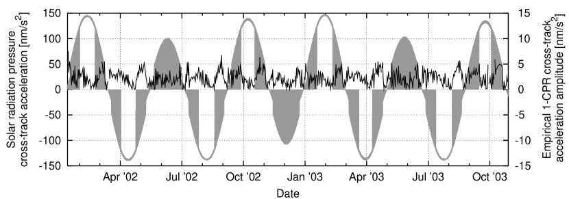
Figure 1: Time series of the modelled Jason–1 out–of–plane solar radiation pressure acceleration (grey) and the estimated 1–cpr out–of–plane acceleration (black).

We have analyzed both the output of the non-gravitational force models described in Berthias et al. (2002) and the resulting residual empirical 1–cpr accelerations estimated from DORIS and SLR tracking over 24–hour intervals. Solar radiation pressure, plotted in Figure 1, is by far the largest out–of–plane non–gravitational acceleration, with a maximum amplitude of 147 nm s^-2. It is followed by Earth radiation pressure at approximately 7 nm s^-2. The contributions of aerodynamic drag and the thermal imbalance force on the cross–track component are both estimated to have a maximum of approximately 0.5 nm s^-2. As can be seen in Figure 1, the cross–track solar radiation pressure acceleration shows a sinusoidal long-term behavior, crossing zero when the Sun–satellite vector is in the orbital plane, roughly every 60 days. It is modulated by the long–term seasonal variations in Sun–Earth geometry, as well as by eclipses and the changing satellite frontal area, both of which contribute 1–cpr variations. In fact, the shading of certain areas in Figure 1 is due to the effect of the eclipses, which, at once–per–orbit, occur much more frequently than can be resolved in Figure 1.

As mentioned before, the empirical 1–cpr accelerations absorb the errors of almost all the unmodelled or mismodelled forces. Now note the systematic way in Figure 1, in which the empirical 1–cpr cross-track acceleration drops to values of below 1 nm s^-2 near the end of each eclipse–free period, and has its maximum level of 5–6 nm s^-2 only during periods containing eclipses. The fact that the amplitude, but also the phase (not shown in Figure 1) of the 1–cpr accelerations show a correlation with the orientation of the orbital plane with respect to the Sun, indicates that it is for a large part absorbing mismodelled radiation pressure accelerations.

By averaging Eq. (9) over one orbital revolution and from the orbital parameters of Table 1 it turns out that a 1–cpr cross–track acceleration would induce a secular rate on the node of Jason proportional to $7.6\times 10^{-5}$ s m${}^{-1}\times S_{N}$ m s^-2. This figure must be multiplied by the combination coefficient $k_{3}$. By using the average value of the empirical 1–cpr acceleration from the above analysis $S_{N}\approx$ 2.3 nm s^-2 as an estimate for the mismodelled non–gravitational forces, it can be argued that the impact on $k_{3}\delta\dot{\Omega}^{\rm Jason-1}$ would amount to 77.4 mas yr^-1.

However, it must be pointed out that our assumed value of $S_{N}$ can be improved by adopting the aforementioned more detailed force models or by tuning the radiation pressure models using tracking data. In addition, it must be pointed out that $S_{N}$ experiences long–term variations mainly induced by the orientation of the orbital plane with respect to the Sun, and the related variations in satellite attitude. For Jason–1 such a periodicity amounts to approximately 120 days (the $\beta^{{}^{\prime}}$ cycle). Let us, now, evaluate what would be the impact of such a long-periodic perturbation on our proposed measurement of the Lense–Thirring effect. Let us write, e.g., a sinusoidal law for the long–periodic component of the weighted nodal rate of Jason–1

$$k_{3}\frac{d\Omega}{dt}=(77.4\ {\rm mas\ yr^{-1}})\times\cos\left[2\pi\left({t\over P_{\rm\beta^{{}^{\prime}}}}\right)\right];$$ (14)

then, if we integrate Eq. (14) over a certain time span $T_{\rm obs}$ we get

$$k_{3}\Delta\Omega=\left({P_{\beta^{{}^{\prime}}}\over 2\pi}\right)(77.4\ {\rm mas\ yr^{-1}})\times\sin\left[2\pi\left({T_{\rm obs}\over P_{\beta^{{}^{\prime}}}}\right)\right].$$ (15)

Then, the amplitude of the shift due to the weighted node of Jason–1, by assuming $P_{\beta^{{}^{\prime}}}\cong 120$ days, would amount to

$$k_{3}\Delta\Omega\leq 4\ {\rm mas}.$$ (16)

The maximum value would be obtained for

$${T_{\rm obs}\over P_{\beta^{{}^{\prime}}}}={j\over 4},\ j=1,3,5,...\cong 30,90,150,...\ {\rm days}.$$ (17)

So, the impact on the proposed measurement of the Lense–Thirring effect would amount to

$$\left.{\delta\mu_{\rm LT}\over\mu_{\rm LT}}\right|_{\rm SRP}\leq{(4\ {\rm mas})\over(49.5\ {\rm mas\ yr^{-1}})\times(T_{\rm obs}\ {\rm yr})};$$ (18)

for, say, $T_{\rm obs}=2$ years Eq. (18) yields an upper bound of $4\%$.

Moreover, it must also be noted that it would be possible to fit and remove such long–periodic signals from the time-series provided that an observational time span longer than the period of the perturbation is adopted.

5 Conclusions

In this paper the use of a suitable linear combination of the nodes of LAGEOS, LAGEOS II, Ajisai and Jason-1 to measure the Lense-Thirring effect in the gravitational field of the Earth is examined. Below we list the major sources of errors along with our evaluations of their impact on the proposed measurement. They are also summarized in Table 5.

5.1 The gravitational error

It turns out that the systematic error of gravitational origin due to the even zonal harmonics can be presently evaluated to be $\sim 1\%$, according to the latest Earth gravity models based on the combined data of CHAMP, GRACE and ground-based measurements. Such an estimate is rather model-independent and will be likely further improved when the new, forthcoming solutions for the terrestrial gravitational potential will be available. The temporal variations of the even zonal harmonics do not represent a major concern because the secular and possible interannual variations of the first three even zonal harmonics are cancelled out, by construction, along with their static components. Moreover, the uncancelled tidal perturbations, like the solar $K_{1}$ tide, vary with relatively high frequencies, so that they could be fitted and removed from the time-series or averaged out over an observational time span of at least 3 years (the longest period is that of the LAGEOS node amounting to 2.84 years).

5.2 The measurement errors

Our largely conservative evaluation for the measurement errors amounts to $\sim 3\%/N$, where $N$ is the number of years of the experiment duration, by assuming a really pessimistic 1 m error in a truly dynamical orbit reconstruction for Ajisai and Jason-1 over the adopted time span.

5.3 The non-gravitational error

In regard to the non-gravitational perturbations, which especially affect Jason-1, it is worthwhile noting that no secular aliasing trends should occur, but only high-frequency harmonic perturbations. However, particular attention should be paid to an as accurate as possible truly dynamical modelling of the non-gravitational accelerations acting on the node of Jason-1. Also a careful choice of the observational time span of the analysis would be required in order to reduce the uncertainties related to the orbital maneuvers which are mainly in plane, although a small, unknown, part of them affects also the out-of-plane part of the orbit. We evaluate the error due to the non-gravitational accelerations as large as $\sim 4\%$ over 2 years.

5.4 Final remarks

In conclusion, the use of the proposed combination, although undoubtedly difficult and demanding, seems to be reasonable and feasible; we give a total root-sum-square uncertainty of $\sim$ 4-5$\%$ over at least 3 years required to average out the uncancelled tidal perturbations. Moreover, the efforts required to perform the outlined analysis should be rewarding not only for the relativists’ community but also for people involved in space geodesy, altimetry and oceanography.

Table 1: Orbital parameters, area-to-mass ratios $S/M$ and Lense-Thirring node precessions $\dot{\Omega}_{\rm LT}$ of LAGEOS, LAGEOS II, Ajisai and Jason-1. $a$ is the semimajor axis, $e$ is the eccentricity and $i$ is the inclination to the Earth’s equator.

	LAGEOS	LAGEOS II	Ajisai	Jason-1
$a$ (km)	12270	12163	7870	7713
$e$	0.0045	0.014	0.001	0.0001
$i$ (deg)	110	52.65	50	66.04
$S/M$ (m2 kg-1)	$6.9\times 10^{-4}$	$7.0\times 10^{-4}$	$5.3\times 10^{-3}$	$2.7\times 10^{-2}$
$\dot{\Omega}_{\rm LT}$ (mas yr-1)	30.7	31.4	116.2	123.4

Table 2: Coefficients $\dot{\Omega}_{.\ell}$ of the classical node even zonal precessions of LAGEOS, LAGEOS II, Ajisai and Jason-1 up to degree $\ell=40$, in mas yr^-1.

$\ell$	LAGEOS	LAGEOS II	Ajisai	Jason-1
2	$4.191586788514\times 10^{11}$	$-7.669274920758\times 10^{11}$	$-3.727536980291872\times 10^{12}$	$-2.527057829772086\times 10^{12}$
4	$1.544030247472\times 10^{11}$	$-5.58637864293\times 10^{10}$	$-1.648980015146924\times 10^{11}$	$-1.993205109225784\times 10^{12}$
6	$3.25092246054\times 10^{10}$	$4.99185703735\times 10^{10}$	$1.549123674154874\times 10^{12}$	$-6.138803379467100\times 10^{11}$
8	$2.1343038821\times 10^{9}$	$1.10707933989\times 10^{10}$	$3.920255674567422\times 10^{11}$	$3.707497244428685\times 10^{11}$
10	$-1.4885315218\times 10^{9}$	$-2.2176133068\times 10^{9}$	$-5.817819204726151\times 10^{11}$	$6.239063727604102\times 10^{11}$
12	$-7.703165634\times 10^{8}$	$-1.1555006405\times 10^{9}$	$-2.971394997875579\times 10^{11}$	$3.963717204418597\times 10^{11}$
14	$-2.097322521\times 10^{8}$	$2.5803602\times 10^{6}$	$1.845822921481368\times 10^{11}$	$7.077668090369869\times 10^{10}$
16	$-3.04891722\times 10^{7}$	$8.81906969\times 10^{7}$	$1.694863702912681\times 10^{11}$	$-1.205024034661577\times 10^{11}$
18	$2.7037212\times 10^{6}$	$1.25437446\times 10^{7}$	$-4.145362988742600\times 10^{10}$	$-1.433538741513498\times 10^{11}$
20	$3.3458376\times 10^{6}$	$-4.8988704\times 10^{6}$	$-8.245022445306935\times 10^{10}$	$-7.489713099273302\times 10^{10}$
22	$1.187265808301358\times 10^{6}$	$-1.666084222225726\times 10^{6}$	$-7.660268981289846\times 10^{8}$	$-1.561231898093660\times 10^{9}$
24	$2.470076374928693\times 10^{5}$	$1.317431893346992\times 10^{5}$	$3.538908387149367\times 10^{10}$	$3.358514735638041\times 10^{10}$
26	$1.550608890427557\times 10^{4}$	$1.463028433008023\times 10^{5}$	$8.354220074961258\times 10^{9}$	$3.149037995362013\times 10^{10}$
28	$-1.163077617533653\times 10^{4}$	$1.121638684708260\times 10^{4}$	$-1.336914484470230\times 10^{10}$	$1.314270726948931\times 10^{10}$
30	$-5.949362622274843\times 10^{3}$	$-9.550578362817516\times 10^{3}$	$-6.639667436677997\times 10^{9}$	$-2.683420483299866\times 10^{9}$
32	$-1.613595912491654\times 10^{3}$	$-2.249168639875042\times 10^{3}$	$4.258273988089967\times 10^{9}$	$-8.603193097267729\times 10^{9}$
34	$-2.333879944573368\times 10^{2}$	$4.033013968161846\times 10^{2}$	$3.832168731738409\times 10^{9}$	$-6.627186370824881\times 10^{9}$
36	$2.133138127038934\times 10^{1}$	$2.311243264675432\times 10^{2}$	$-9.654119269402733\times 10^{8}$	$-2.049870598736127\times 10^{9}$
38	$2.585336000530348\times 10^{1}$	$2.807625658141711$	$-1.872722773415759\times 10^{9}$	$1.220345600570677\times 10^{9}$
40	$9.132066749772124$	$-1.732110087019092\times 10^{1}$	$-9.661717995050006\times 10^{6}$	$2.080653450746944\times 10^{9}$

Table 3: Errors in the even ($\ell=2,4,6...$) zonal ($m=0$) normalized Stokes coefficients $\overline{C}_{\ell 0}=C_{\ell 0}/\sqrt{2\ell+1}$ for various Earth gravity models up to degree $\ell=40$. They are not the formal statistic errors but have been calibrated, although tentatively. Recall that $J_{\ell}\equiv-C_{\ell 0}$. The references for the chosen Earth gravity models solutions are: EIGEN-CG03C (Förste et al. 2005); EIGEN-GRACE02S (Reigber et al. 2005a); EIGEN-CG01C (Reigber et al. 2006); GGM02S (Tapley et al. 2005).

$\ell$	EIGEN-CG03C	EIGEN-GRACE02S	EIGEN-CG01C	GGM02S
2	2.341$\times 10^{-11}$	$5.304\times 10^{-11}$	$3.750\times 10^{-11}$	$1.1\times 10^{-10}$
4	$3.778\times 10^{-12}$	$3.921\times 10^{-12}$	$6.242\times 10^{-12}$	$8.3\times 10^{-12}$
6	$1.840\times 10^{-12}$	$2.049\times 10^{-12}$	$2.820\times 10^{-12}$	$4.5\times 10^{-12}$
8	$1.170\times 10^{-12}$	$1.479\times 10^{-12}$	$1.792\times 10^{-12}$	$2.8\times 10^{-12}$
10	$8.576\times 10^{-13}$	$2.101\times 10^{-12}$	$1.317\times 10^{-12}$	$2.0\times 10^{-12}$
12	$6.847\times 10^{-13}$	$1.228\times 10^{-12}$	$1.053\times 10^{-12}$	$1.8\times 10^{-12}$
14	$5.806\times 10^{-13}$	$1.202\times 10^{-12}$	$8.931\times 10^{-13}$	$1.6\times 10^{-12}$
16	$5.130\times 10^{-13}$	$9.945\times 10^{-13}$	$7.905\times 10^{-13}$	$1.6\times 10^{-12}$
18	$4.684\times 10^{-13}$	$9.984\times 10^{-13}$	$7.236\times 10^{-13}$	$1.6\times 10^{-12}$
20	$4.392\times 10^{-13}$	$1.081\times 10^{-12}$	$6.784\times 10^{-13}$	$1.6\times 10^{-12}$
22	$4.624\times 10{-13}$	$1.026\times 10{-12}$	$7.152\times 10{-13}$	$1.6\times 10^{-12}$
24	$4.912\times 10{-13}$	$9.945\times 10{-13}$	$7.600\times 10{-13}$	$1.7\times 10^{-12}$
26	$5.260\times 10{-13}$	$1.067\times 10{-12}$	$8.148\times 10{-13}$	$1.7\times 10^{-12}$
28	$5.664\times 10{-13}$	$1.150\times 10{-12}$	$8.784\times 10{-13}$	$1.8\times 10^{-12}$
30	$6.140\times 10{-13}$	$1.248\times 10{-12}$	$9.528\times 10{-13}$	$1.9\times 10^{-12}$
32	$6.684\times 10^{-13}$	$1.359\times 10^{-12}$	$1.038\times 10^{-12}$	$1.9\times 10^{-12}$
34	$7.312\times 10^{-13}$	$1.488\times 10^{-12}$	$1.136\times 10^{-12}$	$2.1\times 10^{-12}$
36	$8.028\times 10^{-13}$	$1.635\times 10^{-12}$	$1.248\times 10^{-12}$	$2.4\times 10^{-12}$
38	$8.852\times 10^{-13}$	$1.803\times 10^{-12}$	$1.376\times 10^{-12}$	$2.5\times 10^{-12}$
40	$9.784\times 10^{-13}$	$1.995\times 10^{-12}$	$1.523\times 10^{-12}$	$2.5\times 10^{-12}$

Table 4: Mismodelled combined classical precessions $\left|\left(\dot{\Omega}_{.\ell}^{\rm LAGEOS}+k_{1}\dot{\Omega}_{.\ell}^{\rm LAGEOS\ II}+k_{2}\dot{\Omega}_{.\ell}^{\rm Ajisai}+k_{3}\dot{\Omega}_{.\ell}^{\rm Jason-1}\right)\right|\delta J_{\ell}$, in mas yr^-1, for various Earth gravity models up to degree $\ell=40$. The results of Table 2 and Table 3 have been used. The percent upper bound of the total error $\delta\mu_{\rm LT}$, for a given model, is obtained by summing all the elements of the column corresponding to the model. The result is reported in the last line. The predicted Lense-Thirring slope is 49.5 mas yr^-1.

$\ell$	EIGEN-CG03C	EIGEN-GRACE02S	EIGEN-CG01C	GGM02S
2	-	-	-	-
4	-	-	-	-
6	-	-	-	-
8	0.141	0.178	0.216	0.338
10	0.170	0.417	0.261	0.397
12	0.093	0.168	0.014	0.246
14	0.011	0.023	0.017	0.031
16	0.027	0.052	0.041	0.084
18	0.027	0.058	0.042	0.092
20	0.013	0.032	0.020	0.047
22	$\mathcal{O}(10^{-4})$	$\mathcal{O}(10^{-4})$	$\mathcal{O}(10^{-4})$	$\mathcal{O}(10^{-4})$
24	0.007	0.014	0.011	0.025
26	0.008	0.016	0.012	0.026
28	0.004	0.008	0.006	0.013
30	$\mathcal{O}(10^{-4})$	0.001	0.001	0.003
32	0.003	0.006	0.005	0.009
34	0.002	0.005	0.004	0.008
36	$\mathcal{O}(10^{-4})$	0.002	0.001	0.003
38	$\mathcal{O}(10^{-4})$	0.001	0.001	0.002
40	0.001	0.002	0.002	0.003
$\delta\mu_{\rm LT}\ (\%)$	1.0	1.9	1.3	2.6

Table 5: Error budget. The measurement error goes as 3$\%/N$, where $N$ is the number of years of the observational time span: we assume a $\sim 1$ m rms error over that time interval. A duration of at least 3 years is required to average out the $K_{1}$ solar tide perturbation on the LAGEOS node whose period, equal to that of the satellite’s node, amounts to 2.84 years. The other nodes have shorter periods. The upper limit for the non-gravitational perturbation is over 2 years.

Type of error	geopotential	measurement	non-gravitational
	1$\%$	3$\%$	4$\%$