Revisiting the Light Cone of the Gödel Universe

Abstract

The structure of a light cone in the Gödel universe is studied. We derive the intrinsic cone metric, calculate the rotation coefficients of the ray congruence forming the cone, determine local differential invariants up to second order, describe the crossover (keel) singularities and give a first discussion of its focal points. Contrary to many rotation coefficients, some inner differential invariants attain simple finite standard values at focal singularities.

1 Introduction

Gödel’s rotating cosmological model [12], [13] is one of the most interesting solutions of Einstein’s field equations with negative $\Lambda$-constant, particularly in view of its contribution to our understanding of rotation in relativity and its signs of causality breakdown due to the existence of closed timelike curves [15], [27], [21].

The Gödel solution is also of interest for a study of light ray caustics, which are basic for a discussion of the strong lensing effects in the Universe [28],[25]. There are now many papers discussing singularities on characteristic manifolds of the Einstein field equations, mainly based on powerful mathematical theorems of Lagrangian and Legendrian maps [8],[10],[4], [9], [11]. One may also mention an older article by Laurent, Rosquist and Sviestins [18], where the cone of an Ozsváth class III metric [20] was studied. This metric already includes the Gödel metric as a particular case.

Focal subsets (caustics) are likely to be present on null hypersurfaces, if a weak energy condition holds for its lightlike generators (see [22], [6]), hence almost always in realistic astrophysical or cosmological situations. They have often a complicated structure and are an obstacle for attempts to solve the characteristic initial value problem for Einstein’s field equations numerically, since integration along null geodesics runs into difficulties at caustics [8], [10],[29]. It would be extremely helpful if existent algorithms could be modified or replaced to allow numerical processing through such singularities. A preliminary step is to study caustics in exact solutions of the field equations.

In this connection the Gödel light cone could be a useful object, since here the behaviour of light rays is already sufficiently complex to give an impression of features which we can expect in more realistic geometries, and on the other side it is simple enough to allow a complete analytical treatment. Due to the five-dimensional group of isometries admitted by the Gödel metric, which has a four-dimensional transitive subgroup, all light cones have the same internal structure.

A first discussion of the inner geometry of the Gödel cone was given by us in 1972 [1], [2], based on the integration of geodesics performed by Kundt in 1956 [17]. Use of computer based formula manipulation technique has shown, that a number of complicated relations can be simplified considerably. In particular, the structure of caustics and the resulting startling cyclic lens effects found in [1] and [2] now became more transparent. The lens effects arise from a quasi-periodic re-focussing of the generators and are surprisingly similar to those discussed by Ozsváth and Schücking for the light cone of a plane gravitational wave propagating in vacuum, one of their anti-Mach metrics [19].

We apply the geometrical decription of null hypersurfaces developped in [6],[7]. After integrating the null geodesics in Section II, we derive the intrinsic metric of the Gödel cone in Section III, calculate and discuss its rotation coefficients and differential invariants in Section IV and turn to a description of caustics in Section V. While rotation coefficients of the light ray congruence forming the cone have as a rule singularities on focal surfaces or keel points, some local inner differential invariants have simple finite limits there. It is interesting that this feature - with the same asymptotic values of invariants at singularitites - has shown up in all nontrivial light cones studied so far by us. A method to relate intrinsic cone coordinates to the angles $(\theta,\phi)$ on the observer sky is described in an Appendix.

2 Light rays in the Gödel universe

2.1 General Congruence

Gödel’s stationary solution of Einstein’s field equations with cosmological constant describes the gravitational field of a uniform distribution of rotating dust matter, where - loosely speaking - the gravitational attraction of matter and the added attractice force of a negative $\Lambda$-constant is compensated by the centrifugal force of rotation. Hawking and Ellis [15] introduce the Gödel metric with the coordinates $t,x,\bar{y},z$ as (we have exchanged $x,y$ to reach conformity with our notation, the signature will be taken as (-1,1,1,1), and the conventions of the Misner-Thorne-Wheeler book will be adopted):

$$ds^{2}=-dt^{2}+d\bar{y}^{2}-\frac{1}{2}e^{2\bar{y}/b}dx^{2}+dz^{2}-2e^{\bar{y}/b}dtdx.$$

The matter density is given by $\kappa\mu=-2\Lambda=1/b^{2}$. With $y=\sqrt{2}be^{-\bar{y}/b}$ one obtains the form of the metric used in [2] and employed also here:

$$ds^{2}=-(dt+\frac{\sqrt{2}b}{y}dx)^{2}+\frac{b^{2}}{y^{2}}(dx^{2}+dy^{2})+dz^{2}$$ (1)

As first shown by Kundt [17], the differential equations $x^{\prime\prime\mu}+\Gamma^{\mu}_{\rho\sigma}x^{\rho}{{}^{\prime}}x^{\sigma}{{}^{\prime}}=0$ for the geodesics admit the first integrals

$$t^{\prime}\equiv x^{(0)}{{}^{\prime}} = (-c_{2}/\sqrt{2}+\sqrt{2}y)/c_{0},$$ (2)

$$x^{\prime}\equiv x^{(1)}{{}^{\prime}} = y(c_{2}-y)/(bc_{0}),$$ (3)

$$y^{\prime}\equiv x^{(2)}{{}^{\prime}} = y(x-c_{1})/(bc_{0}),$$ (4)

$$z^{\prime}\equiv x^{(3)}{{}^{\prime}} = c_{3}/c_{0},$$ (5)

Here the prime denotes the derivative with respect to a running parameter $s$ on the geodesic, i.e., $s$ is the proper time or invariant length for a non-null geodesic and an affine parameter for light rays. The integrals depend on four parameters $c_{0},c_{1},c_{2},c_{3}$ and are subject to the normalization condition $g_{\mu\nu}x^{\mu}{{}^{\prime}}x^{\nu}{{}^{\prime}}=constant$, where the constant is -1 for a timelike, 1 for a spacelike and 0 for a null geodesic. For the null geodesics discussed here, different values of $c_{0}$ correspond only to different definitions of the affine parameter, so we assume $c_{0}=1$ subsequently. With (2)-(5), the normalization condition becomes for null geodesics

$$(x-c_{1})^{2}+(y-c_{2})^{2}=\frac{1}{2}c_{2}^{2}-c_{3}^{2}\equiv c_{4}^{2},$$ (6)

thus the projection of null geodesics into the $xy$-plane are confined to a circle with radius $|c_{4}|$. Light can move to arbitrary large distances only in the $z$-direction, the direction of the rotation axis. Equation (6) is solved with

$$x=c_{1}+c_{4}\sin{\Phi},~{}y=c_{2}+c_{4}\cos{\Phi},$$ (7)

where $\Phi(s)$ is an unknown function. Since $y\geq 0$, no circle point can lie below the $y$-axis. The parameter range for null geodesics is thus constrained by

$$c_{2}\geq\sqrt{2}|c_{4}|,$$ (8)

corresponding to points below the line $ACD$ in the upper half plane and above the line $AEF$ in the lower half plane of Fig. 1.

(3) and (4) lead to a single differential equation for $\Phi:$

$$b\Phi^{\prime}+c_{4}\cos{\Phi}+c_{2}=0.$$ (9)

We first shortly discuss the particular case $c_{4}=0$, when the circle in the $xy$-plane shrinks to a point. Here (2)-(5) have the solution

$$t=\frac{c_{2}}{\sqrt{2}}s+t_{0},~{}x=c_{1},~{}y=c_{2},~{}z=\frac{c_{2}}{\sqrt{2}}s+z_{0},$$ (10)

thus through every point $P$ of the Gödel universe passes one exceptional light ray: It is the light ray sent or received by a comoving observer at $P$ in or opposite to the direction of the local rotation axis. Returning to the general case, integration of (9) gives with an integration constant $k_{1}$

$$\tan{\frac{\Phi}{2}}=-\sqrt{\frac{c_{2}+c_{4}}{c_{2}-c_{4}}}\tan{(\sqrt{c_{2}^{2}-c_{4}^{2}}\frac{s+k_{1}}{2b})}.$$ (11)

The inequality (8) ensures that the roots are real. To simplify the representation, we define a new real constant $k$

$$k=\frac{k_{1}}{2b}\sqrt{c_{2}^{2}-c_{4}^{2}},$$ (12)

and introduce a new affine parameter $w$ instead of $s$:

$$w=\frac{s}{2b}\sqrt{c_{2}^{2}-c_{4}^{2}}.$$ (13)

Integrating also the remaining equations (2),(5), one finally obtains ($\epsilon=\pm 1$, since $c_{3}$ can have both signs)

$$t(w) = 2\sqrt{2}b\arctan{(\sqrt{\frac{c_{2}+c_{4}}{c_{2}-c_{4}}}\tan{(w+k)})}-\frac{\sqrt{2}bc_{2}w}{\sqrt{c_{2}^{2}-c_{4}^{2}}}+c_{5},$$ (14)

$$x(w) = c_{1}-\frac{c_{4}\sqrt{c_{2}^{2}-c_{4}^{2}}\sin{(2w+2k)}}{c_{2}-c_{4}\cos{(2w+2k)}},$$ (15)

$$y(w) = \frac{c_{2}^{2}-c_{4}^{2}}{c_{2}-c_{4}\cos{(2w+2k)}},$$ (16)

$$z(w) = \sqrt{2}\epsilon bw\frac{\sqrt{c_{2}^{2}-2c_{4}^{2}}}{\sqrt{c_{2}^{2}-c_{4}^{2}}}+c_{6}$$ (17)

as parameter representation of the null geodesics. Counting the number of independent parameter one sees that (14)-(17) is the generic null congruence of the Gödel cosmos. Its explicit form helps to answer questions on null geodesics in the Gödel cosmos. For example, one can easily conclude that there are no closed null geodesics, which would require $x^{\mu}(w)=x^{\mu}(w_{1})$ for some values $w$ and $w_{1}$: Taking first $\mu=3$, Equation (17) shows that $c_{3}=0$ or $c_{2}=\sqrt{2}c_{4}$ is needed, which corresponds to $z=const$. An inspection of the relation for $\mu=1,2$ shows, that these relations can be satisfied by means of periodic functions. Thus a subset of null geodesics may return to the same space point, but the point is (repeatedly) reached at different times $t$, due to the aperiodic term proportional to $w$ in (14).

2.2 Light cone geodesics

We are here interested in those null geodesics, which form a cone with the vertex at a point $P_{0}$ with the coordinates $(0,0,b,0)$, say. $P_{0}$ corresponds to the origin of the Hawking-Ellis coordinates. Since all light cones of the Gödel cosmos have the same intrinsic structure, we could have chosen any other origin in principle. Furthermore, for definiteness, the past cone ($w>0$) will be considered. Assuming $w=0$ at the vertex, we have four relations which will be used to determine $c_{1},c_{5},k$ and $c_{6}$ in terms of the remaining parameters $c_{2}$ and $c_{4}$:

$$c_{1} = \frac{c_{4}\sqrt{c_{2}^{2}-c_{4}^{2}}\sin{2k}}{c_{2}-c_{4}\cos{2k}},$$ (18)

$$c_{5} = -2b\sqrt{2}\arctan{(\sqrt{\frac{c_{2}+c_{4}}{c_{2}-c_{4}}}\tan{k}}),$$ (19)

$$\cos{2k} = \frac{c_{4}^{2}-c_{2}^{2}+bc_{2}}{bc_{4}},$$ (20)

$$c_{6} = 0.$$ (21)

The requirement that the $c_{1},c_{5},k$ and $c_{6}$ exist and are real restricts $c_{2}$ and $c_{4}$ beyond (8). In [1],[2] a pair $(u,v)$ of transversal parameters was introduced to replace $(c_{2},c_{4})$:

$$u^{2}=\frac{c_{4}+c_{2}-b}{c_{4}-c_{2}+b},~{}v^{2}=\frac{c_{2}+c_{4}}{c_{2}-c_{4}}.$$ (22)

Inverting, we have

$$c_{2}=\frac{b(1+u^{2})(v^{2}+1)}{2(u^{2}+v^{2})},~{}c_{4}=\frac{b(1+u^{2})(v^{2}-1)}{2(u^{2}+v^{2})}.$$

The map $(c_{2},c_{4})\rightarrow(u,v)$ is not everywhere regular, since the functional determinant $\frac{\partial c_{2}}{\partial u}\frac{\partial c_{4}}{\partial v}-\frac{\partial c_{2}}{\partial v}\frac{\partial c_{4}}{\partial u}=-2uvb^{2}\frac{(u^{2}+1)(v^{2}-1)}{u^{2}+v^{2}}$ has for real $u,v$ zeros at $u=0,v=0,v^{2}=1$. The first two arise from using squares on the lhs of (22), the singularity $v^{2}=1$ or $c_{4}=0$ corresponds to the exceptional ray introduced above. In terms of $u$ and $v$, (20) can be written $\cos{2k}=\frac{v^{2}-u^{2}}{v^{2}+u^{2}}$. It is seen from this equation, that $u^{2}$ cannot be negative for geodesics forming the $P_{0}$-cone, this also applies to $v^{2}$ because of (8). Thus $u$ and $v$ as introduced by (22) are real.

For more information we refer to Fig. 1.

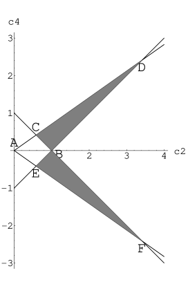
Figure 1:  

$c_{2}$-$c_{4}$-parameter plane for null geodesics in the Gödel universe ($b=1$ assumed). Null geodesics have their integration constants $c_{2}$ and $c_{4}$ between the lines $ACD$ and $AEF$. Those forming the (past) light cone through $P_{0}$ are confined to the shadowed triangles, with $c_{4}>0$ for the western hemisphere and $c_{4}<0$ for the eastern hemisphere of the observer sky. But only the northern hemisphere is mapped 1:1 to the two triangle regions, for the missing southern hemisphere a second copy of the figure is needed. To obtain the topology of a sphere, certain boundary lines of the triangles in both copies must be identified pointwise. The lines $CD$ and $EF$ correspond to parts of the equator, the pole ray at $B$ is the exceptional ray towards the rotation direction.

In this parameter plane the points $A$ through $F$ correspond to coordinate pairs $(c_{2},c_{4})$ given by

$$A=(0,0),~{}~{}B=b(1,0),~{}~{}C=b(\frac{\sqrt{2}}{\sqrt{2}+1},\frac{1}{\sqrt{2}+1}),~{}~{}D=b(\frac{\sqrt{2}}{\sqrt{2}-1},\frac{1}{\sqrt{2}-1}),$$

$$E=b(\frac{\sqrt{2}+2}{\sqrt{2}+1},-\frac{1}{\sqrt{2}+1}),~{}~{}F=b(\frac{\sqrt{2}}{\sqrt{2}-1},-\frac{1}{\sqrt{2}-1}).$$

Allowed parameters $c_{2},c_{4}$ for generators are subject to (8), and lie above the line $AEF$ as well as below the line $ACD$. $v=const$ is the equation of straight lines (”parallels”) starting at $A$, with $v$ ranging from $v=1$ (the $c_{2}$-axis) to $v=1+\sqrt{2}$ (the line $ACD$) in the upper half plane. For $v<1$ the lines $v=const$ lie in the lower half plane $c_{4}<0$, ranging from $v=1$ through $v=1/(1+\sqrt{2})$ (the line $AEF$). Curves with $u=const$ are straight lines (”meridians”) through the point $B$, ranging from $u=0$ ($BC$) to $u\rightarrow\infty$ ($BD$) in the upper half plane. We shall find it appropriate (Appendix B) to take $u$ negative in one hemisphere. As discussed subsequently, the cone generators cover the two shadowed triangles in Fig 1, which correspond to certain quadrants on the observer sky, e.g., the lines $EF$ and $CD$ form part of the equator. Two copies of the figure are required to cover the full observer sphere. For details we refer to Appendix B.

Returning to the cone representation, the parameters $c_{5},c_{1},k$ and $c_{6}$ can be written in terms of $u$ and $v$ in a compact form as solutions of (18)-(21):

$$c_{1} = -b\frac{u(1-v^{2})}{u^{2}+v^{2}},$$

$$c_{5} = -2\sqrt{2}b\arctan{u},$$

$$\tan{k} = \frac{u}{v},$$

$$c_{6} = 0.$$

Substituting these values into (2)-(5), one obtains as a parameter representation of the light cone through $P_{0}$:

$$\qquad t = t(u,v,w)=-\frac{bw}{\sqrt{2}}(v+\frac{1}{v})+2\sqrt{2}b\arctan{\frac{(u^{2}+v^{2})\tan w}{v(u^{2}+1)+u(v^{2}-1)\tan(w)}},$$ (23)

$$\qquad x = x(u,v,w)=b(v^{2}-1)\frac{\sin{w}(v(u^{2}-1)\cos{w}+u(v^{2}+1)\sin{w})}{(v\cos{w}-u\sin{w})^{2}+v^{2}(u\cos{w}+v\sin{w})^{2}},$$ (24)

$$\qquad y = y(u,v,w)=\frac{bv^{2}(u^{2}+1)}{(v\cos w-u\sin w)^{2}+v^{2}(u\cos w+v\sin w)^{2}},$$ (25)

$$\qquad z = z(u,v,w)=\frac{b\epsilon w}{\sqrt{2}v}\sqrt{6v^{2}-1-v^{4}}.$$ (26)

Positive values of the affine parameter $w$ correspond to the past light cone, negative values to the future cone. The sign $\epsilon$ distinguishes between the northern ($\epsilon=1$) and southern ($\epsilon=-1$) hemisphere of the observer sky. We note the following invariance property of the system (23)-(26): Substituting $-1/u$ for $u$ and $1/v$ for $v$ leads to the same geodesics:

$$x^{\mu}(u,v,w)=x^{\mu}(-\frac{1}{u},\frac{1}{v},w)$$ (27)

The same map sends also $(c_{2},c_{4})$ into $(c_{2},-c_{4})$. Some geodesics of the parallel $v=1.5$ are plotted in Fig. 2.

Figure 2:  

The twisted generators of the past light cone through $P_{0}$ are shown in a fictitious Euklidean 3-space ${\cal R}^{3}$. Plotted are the coordinates $x(u,v,w),y(u,v,w),t(u,v,w)$ from (23)-(25) for rays on the parallel $v=1.5$ and several $u$ with constant separation $\pi/30$ in the meridian angle $\phi=2\arctan{u}$ corresponding to $u$. The $z$-coordinate is suppressed, keels appear as points, focal surfaces as lines. The affine parameter ranges from $w=0$ at the vertex (top) to $w=1.5\pi$ (bottom), the plot ends before the second keel line at $w=2\pi$ is reached.- Distances cannot be represented correctly in such a projection, the type of caustics is preserved however, since the map from the curved $V^{3}$ to ${\cal R}^{3}$ is a diffeomorphism.

Knowing the tangential vector $\frac{dx^{\mu}}{dw}$ of the past light cone from (23)-(26) or from (2)-(5), one can calculate the redshift $z$ of distant objects from the well-known relation

$$1+z=\frac{(\frac{dx^{\mu}}{dw}V^{\nu}g_{\mu\nu})_{emitter}}{(\frac{dx^{\mu}}{dw}V^{\nu}g_{\mu\nu})_{observer}}.$$

With $V^{\mu}=\delta^{\mu}_{0}$ and (23)-(26) one finds $z=0$: As noted already by Gödel in his original paper [12], distant objects comoving with the cosmic fluid would show no redshift, proving that this model cannot represent the real Universe.

3 Light cone metric

The spacetime coordinates of light-rays through $P_{0}$, (23)-(26), depend on the affine parameter $w$ as well as on two quantities $u,v$. While $w$ determines a position on a light ray, $u$ and $v$ label a ray. The tripel $w^{i}\equiv(w,u,v)$ may therefore be used as intrinsic coordinates on the cone. Below we will see how $u$ and $v$ are related to the angles $\theta,\phi$ on the sky of a comoving observer at $P_{0}$, who wants to fix an event on his past light cone. The intrinsic three-dimensional metric of the light cone at $P_{0}$ can be found from (23)-(26) by means of

$$\gamma_{ik}=g_{\mu\nu}\frac{\partial x^{\mu}}{\partial w^{i}}\frac{\partial x^{\mu}}{\partial w^{k}},$$

where $w^{i}=(w,v,u)$. Since $\frac{\partial x^{\mu}}{\partial w}$ is the tangential vector to the cone and hence null, the components of the cone metric can be reduced to a two-dimensional metric $\gamma_{AB}$:

$$\gamma_{00} = 0,$$ (28)

$$\gamma_{0A} = 0,$$ (29)

$$\gamma_{22} = \frac{b^{2}}{v^{4}f_{2}}(w^{2}f_{1}^{4}+2wf_{2}f_{1}^{2}\sin{w}\cos{w}+f_{2}^{2}\sin^{2}{w}+f_{2}f_{1}^{2}\sin^{4}{w}),$$ (30)

$$\gamma_{23} = \frac{b^{2}f_{1}^{3}\sin^{2}{w}(w-\sin{w}\cos{w})}{v^{4}(u^{2}+1)},$$ (31)

$$\gamma_{33} = \frac{b^{2}f_{1}^{2}\sin^{2}{w}(4v^{2}-f_{1}^{2}\sin^{2}{w})}{v^{4}(u^{2}+1)^{2}},$$ (32)

where we have introduced the two functions

$$f_{1}(v)=v^{2}-1,~{}f_{2}(v)=6v^{2}-1-v^{4},$$ (34)

which are useful to compactify expressions.

In general, the $\gamma_{AB}$ form an one-dimensional sequence of positive-definite two-dimensional metrics on the cone, parametrized by the affine parameter $w$. They represent metric spheres in the neighbourhood of the vertex $w=0$, but become progressively deformed for increasing parameters $w$. On some subsets of the cone the inner metric degenerates additionally, i.e. the two-dimensional determinant $\gamma$ becomes zero. This signifies an intersection of light rays forming the cone, if the zero of $\gamma$ is not caused by a coordinate singularity. In focal points or caustics geodesics with infinitesimally differing values of $u,v$ meet, while in crossover or keel points (we have taken the latter notation from a paper by M. Riesz [26]) the intersecting geodesics may have quite different transversal parameters. Sets of focal points form in general two-dimensional focal surfaces on a null hypersurface. For the Gödel cone the determinant $\gamma$ can be represented in a compact form:

$$\gamma \equiv |\gamma_{AB}|=h^{2},$$ (35)

$$h \equiv \frac{2b^{2}f_{1}p(v,w)\sin{w}}{(u^{2}+1)\sqrt{f_{2}}v^{3}},$$ (36)

$$p(v,w) \equiv f_{1}^{2}w\cos{w}+f_{2}\sin{w}$$ (37)

(abbreviations are deliberately chosen in this paper to compactify expressions). The simple expression for $\gamma$ allows to pick up the cone singularities easily. Apart from the vertex $w=0$, $\gamma$ vanishes periodically for $w=n\pi$, $n$ an integer, which is similar to the behaviour of light cones in a closed Robertson-Walker model with the time extended to several cycles. But contrary to the RW case, the two-dimensional spacelike surfaces $w=const$ do not shrink to points at $w=n\pi,~{}n\neq 0$, but rather to spacelike lines, the keel lines, discussed in Section V. Further zeros of $\gamma$ are given by $p(v,w)=0$, which is the equation of the focal surfaces, also discussed in Section V. The remaining zeros of $\gamma$ are given by $f_{1}=0$ or $v=1$, corresponding to the exceptional pole rays, and $u\rightarrow\infty$. The latter is related to a coordinate singularity.

For later use it is appropriate to introduce a second function $q(v,w)$, with the property of being not negative:

$$q(v,w)\equiv 4(1+f_{1})-f_{1}^{2}\sin^{2}{w}.$$ (38)

$q$ vanishes if and only if $f_{2}/f^{2}_{1}=-\cos^{2}{w}$. Since the lhs is not negative, the condition $q=0$ holds only for $\cos{w}=0$ (or $w=(1+2n)\pi/2$, $n$ integer), and for $f_{2}=0$, or $v=1+\sqrt{2}$. Since at these points also $p=0$, the equation $q=0$ represents curves on the light cone, where the equator rays $v=1+\sqrt{2}$ meet the $n$th focal surface (Section IV). With $q$, the intrinsic cone metric can also be written as

$$\gamma_{22} = \frac{b^{2}}{v^{4}f_{2}\cos^{2}{w}}(p^{2}-2pf_{2}\sin^{3}{w}+qf_{2}\sin^{4}{w}),$$ (39)

$$\gamma_{23} = \frac{b^{2}f_{1}\sin^{2}{w}}{v^{4}(u^{2}+1)\cos{w}}(p-q\sin{w}),$$ (40)

$$\gamma_{33} = \frac{b^{2}f_{1}^{2}\sin^{2}{w}}{v^{4}(u^{2}+1)^{2}}q,$$ (41)

allowing to check easily that the rank of $\gamma_{ik}$ indeed becomes 1 (i.e. $|\gamma_{AB}|=0$, but not all $\gamma_{AB}=0$) at caustics $p=0$.

The range and the geometrical meaning of the transversal cone coordinates $u$ and $v$ must now be discussed. Apparently, $u$ may take all values out of the range $(-\infty,\infty)$. For a real $z$-coordinate the function $f_{2}=6v^{2}-1-v^{4}$ cannot have negative values, so $v$ is restricted to an interval $(v_{min},v_{max})$ where $v_{min}=1/(1+\sqrt{2})$ and $v_{max}=1+\sqrt{2}$. If $v$ belongs to this range, also $1/v$ does. However, the substitution (27) shows that two different pairs $(u,v)$ might represent the same null geodesic. Also two different geodesics might be represented by the same $(u,v)$-pair.

A natural way to parametrize a light cone is to take the angular coordinates $(\theta,\phi)$ at the sky of an observer sitting at the vertex and comoving with the fluid. As usual, $\theta$ ranges from $0$ (north pole) to $\pi$ (south pole), and $\phi$ from $0$ to $2\pi$. To find the relation between the sky coordinates and $(u,v)$ we have used a method, which is exclusively based on the intrinsic cone metric. Leaving the details for Appendix B, the result is

$$\qquad u^{2}=\frac{1-\cos{\phi}}{1+\cos{\phi}},\quad v^{2}=\frac{\sqrt{2}+\sin{\theta}}{\sqrt{2}-\sin{\theta}},\quad\cos{\phi}=\frac{1-u^{2}}{1+u^{2}},\quad\sin{\theta}=\sqrt{2}\frac{v^{2}-1}{v^{2}+1}.$$ (42)

$u$ ranges from $u=0$ for $\phi=0$ to $\infty$ at $\phi=\pi$, jumps there to $-\infty$, and increases to zero at $\phi=2\pi$. $v$ starts from $v=1$ at the north pole ($\theta=0$), increases to $v_{max}=1+\sqrt{2}$ at the equator ($\theta=\pi/2$), and decreases to $1$ at the south pole ($\theta=\pi$). As explained in the Appendix, only the partial interval $(1,v_{max})$ is used for $v$. A point on the sphere is fixed by a pair $(u,v)$ together with the sign of $\epsilon$. This ensures that a pair $(u,v)$ from the $u$-range $(-\infty,\infty)$ and $v$-range $(1,v_{max})$ is a one-two-one map of the light rays in the northern resp. southern hemisphere. The exceptional ray with $v=1,\epsilon=1$ corresponds to the north pole, the antipodal ray with $v=1,\epsilon=-1$ to the south pole.

Transforming the inner metric $\gamma_{ik}$ to angular coordinates $\theta,\phi$ does not simplify neither its form nor other relations very much, so we continue to work with $u$ and $v$ as transversal coordinates.

In the chosen representation the equator is given by $v=v_{max}=1+\sqrt{2}$ and geodesics sent out in these directions (orthogonal to the rotation axis) lie always in the plane $z=0$. Since here $f_{2}=0$, the cone metric becomes singular, its determinant $\gamma$ tends to infinity. This is a coordinate singularity: The angular coordinates are regular along the equator, but the functional determinant $|\frac{\partial(\theta,\phi)}{\partial(v,u)}|$ suffers from a diverging factor $f_{2}^{-1/2}$. If carefully treated, this divergence will not cause trouble.

4 Rotation coefficients and invariants

4.1 Geometries on null hypersurfaces

The local differential geometry of null hypersurfaces such as a cone was in some detail described in [6] and [7], see also [24],[23]. We summarize the points most important for us. This geometry is formulated in terms of the rotation coefficients of a certain class of triads, defined as follows: At every regular point $P$ of the cone there exists a unique direction $\epsilon^{i},~{}i=1,2,3$, the direction of the null geodesic passing that point. $\epsilon^{i}$ satisfies $\gamma_{ik}\epsilon^{k}=0$ and is given up to a factor by $\epsilon^{i}=\delta^{i}_{1}$ in the coordinate system $(u,v,w)$ used in the last section. The two other directions, which are spacelike in regular points and orthogonal to each other, may be combined linearly to form a complex vector $t^{i}$. We have $t^{i}\epsilon^{k}\gamma_{ik}=0$ and normalize $t^{i}$ such that $t^{i}t^{k}\gamma_{ik}=0,~{}t^{i}\bar{t}^{k}\gamma_{ik}=1$. The transversal directions $t^{i}$ are determined only up to a transformation $t^{\prime i}=e^{i\omega}(t^{i}-\bar{\kappa}\epsilon^{i})$, $\omega$ real and $\kappa$ complex. Note that $\epsilon^{i}$ is also subject to a change $\epsilon^{\prime i}=\lambda\epsilon^{i}$ ($\lambda$ real), since the running parameter along a ray may be chosen arbitrarily (it need not to be an affine parameter). The covariant components of the transversal directions are given by $t_{i}=\gamma_{ik}t^{k}$ and $\gamma_{i}$, where $\gamma_{i}$ is defined by $t^{i}\gamma_{i}=0,~{}\epsilon^{i}\gamma_{i}=1$. This completes the covariant triad. The rotation coefficients divergence $\rho$, shear $\sigma$ as well as other coefficients are given in terms of the derivatives of the triad:

$$\rho+i\upsilon = \epsilon^{i}t^{k}(\bar{t}_{i,k}-\bar{t}_{k,i}),$$ (43)

$$\sigma = \epsilon^{i}\bar{t}^{k}(\bar{t}_{i,k}-\bar{t}_{k,i}),$$ (44)

$$\tau = \bar{t}^{i}t^{k}(\bar{t}_{i,k}-\bar{t}_{k,i}),$$ (45)

$$\chi = \frac{1}{2}\bar{t}^{i}\epsilon^{k}(\gamma_{i,k}-\gamma_{k,i}),$$ (46)

$$i\varphi = \frac{1}{2}\bar{t}^{i}t^{k}(\gamma_{i,k}-\gamma_{k,i}).$$ (47)

$\tau$ is related to the intrinsic geometry of the two-dimensional wave surfaces $w=const$, with $w$ here as an affine parameter of the generating null geodesics. The coefficients $\chi$ and $\varphi$ reflect properties of the triad, which are geometrically not relevant. In particular, if $\gamma_{i}$ is chosen as gradient, as we will do here for simplicity, both $\chi$ and $\varphi$ are zero. A change of the triad

$$t^{\prime}_{i}=e^{i\omega}t_{i},~{}\gamma^{\prime}_{i}=\frac{1}{\lambda}\gamma_{i}+\kappa t_{i}+\bar{\kappa}\bar{t}_{i},~{}t^{\prime i}=e^{i\omega}(t^{i}-\bar{\kappa}\lambda\epsilon^{i}),~{}\epsilon^{\prime i}=\lambda\epsilon^{i}$$

produces a change of the rotation coefficients as follows:

$$\rho^{\prime} = \lambda\rho,$$

$$\sigma^{\prime} = \lambda e^{-2i\omega}\sigma,$$

$$\tau^{\prime} = e^{-i\omega}(\tau+i\bar{\delta}\omega-i\kappa\lambda D\omega-i\kappa\lambda\upsilon+\bar{\kappa}\lambda\sigma-\kappa\lambda\rho),$$

$$\upsilon^{\prime} = \lambda(\upsilon+D\omega),$$

$$\chi^{\prime} = \frac{1}{2}e^{-i\omega}(2\chi+\frac{\bar{\delta}\lambda}{\lambda}-\kappa\rho\lambda+i\upsilon\kappa\lambda-\bar{\kappa}\lambda\sigma+\lambda D\kappa),$$

$$i\varphi^{\prime} = \frac{1}{\lambda}i\varphi+\frac{1}{2}(\bar{\kappa}\tau-\kappa\bar{\tau}+\delta\kappa-\bar{\delta}\bar{\kappa})$$

$$+\frac{1}{2}\kappa(2\bar{\chi}+\frac{\delta\lambda}{\lambda}-i\bar{\kappa}\lambda\upsilon-\kappa\lambda\bar{\sigma}+\lambda D\bar{\kappa})$$

$$-\frac{1}{2}\bar{\kappa}(2\chi+\frac{\bar{\delta}\lambda}{\lambda}+i\kappa\lambda\upsilon-\bar{\kappa}\lambda\sigma+\lambda D\kappa).$$

The last two equations show that $\chi=0$ and $\varphi=0$ are preserved for $\kappa,\lambda$ satisfying $\delta\kappa-\bar{\delta}\bar{\kappa}+\bar{\kappa}\tau-\kappa\bar{\tau}=0,~{}\delta\lambda/\lambda^{2}+D\bar{\kappa}-\bar{\kappa}(\rho+i\nu)-\kappa\bar{\sigma}=0$. Coordinate invariant statements are formulated in terms of those functions of the rotation coefficients and their derivatives, which are invariant with respect to the allowed transformations of the triad. The group of allowed triad transformations defines the type of null surface geometry in the spirit of Felix Klein’s ”Erlangen program” [16]. The most important geometries are the just outlined inner geometry and the affine geometry, where the concept of an affine parameter for the rays is given as additional geometrical element. For other geometries on null hypersurfaces and for more details we refer to [6] or [7], and for a similar definition of null surface geometries the papers by Penrose [24], [23] should be consulted.

4.2 Application to the Gödel cone

We first determine the rotation coefficients for the Gödel cone. The divergence is calculated from $\rho=-\frac{1}{4\gamma}\frac{\partial\gamma}{\partial w}$ and may be written as

$$\rho=-\cot{2w}-\frac{q}{2p\cos{w}},$$ (48)

with the functions $p(v,w),q(v,w)$ defined by (37),(38). The divergence tends to $\pm\infty$ at $w=n\pi$ (keels) and $p=0$ (focal surfaces) and becomes zero at the two-dimensional surfaces

$$-\frac{\tan{2w}}{2w}=\frac{f_{1}^{2}}{f_{2}}$$ (49)

between focal surfaces and keels: Since the rhs of this equation is not negative, the range of $w$, where $\rho=0$ is possible, and hence the position of a zero-divergence surface, is restricted by the condition

$$(2m-1)\frac{\pi}{4}\leq w\leq m\frac{\pi}{2},~{}~{}m=1,2,3....$$ (50)

The amount of shear follows most easily from another general relation $|\sigma|^{2}=\rho^{2}-det(\frac{\partial\gamma_{AB}}{\partial w})/(4\gamma)$:

$$\qquad|\sigma|^{2}=\frac{q^{2}}{4p^{2}\cos^{2}{w}}+\frac{8v^{2}\cos^{2}{w}+q(2\sin^{2}{w}-3)}{2p\sin{w}\cos^{2}{w}}+\frac{1}{4\sin^{2}{w}\cos^{2}{w}}-\frac{f_{1}^{2}}{4v^{2}}.$$ (51)

Like the divergence, also the shear goes to infinity at focal surfaces and keels. The remaining nonvanishing coefficients may be calculated from (43)-(45), the details are given in Appendix A. Splitting $\sigma$ into real and imaginary parts, $\sigma=\sigma_{1}+i\sigma_{2},$ one obtains

$$\sigma_{1} = -\frac{1}{\sin{2w}}+\frac{f_{1}^{2}\sin{2w}}{2q}+\frac{q}{2p\cos{w}},$$ (52)

$$\sigma_{2} = \frac{f_{1}^{2}\sqrt{f_{2}}\sin^{2}{w}}{2vq},$$ (53)

$$\nu = -\frac{f_{1}^{2}\sqrt{f_{2}}\sin^{2}{w}}{2vq},$$ (54)

$$\tau = \frac{i\sqrt{f_{2}}(v^{2}+1)(2v^{2}-f_{1}^{2}\sin^{2}{w})}{bf_{1}p\sqrt{2q}}.$$ (55)

The triad has been chosen so that the resulting rotation coefficients look as simple as possible. There exists in general one (and only one) first-order inner invariant of a null hypersurface, i.e. an invariant function formed from the rotation coefficients alone, without derivatives. This is the quantity $j=\frac{\rho}{|\sigma|}$ or any function of $j$. It is useful to consider $1/j^{2}$, which measures the anisotropic behaviour of the generators around a given one:

$$1/j^{2}=\frac{pf_{1}^{2}(4v^{2}\sin{w}-p)\sin^{2}{w}\cos^{2}{w}+v^{2}(p-q\sin{w})^{2}}{v^{2}(p(2\sin^{2}{w}-1)-q\sin{w})^{2}}.$$ (56)

At caustics $p=0$ (and keel points with $w=n\pi$) this gives $j^{2}=1$ or $j=\pm 1$, depending on the sign of $\rho$. Along the two exceptional rays (pole rays) the shear vanishes and the anisotropy measure $1/j^{2}$ is zero, in accordance with the symmetry properties of the cone.

From the rotation coefficients and their derivatives one may also form some second-order invariants. The purely transversal projections of the four dimensional Ricci and Weyl tensor into the cone are closely related to them. The Ricci and Weyl tensor projections are -without any addition of further embedding quantity- equal to similar projections related to an intrinsic Riemann tensor $R_{ikl}^{~{}~{}m}$ of the null hypersurface,

$$t^{k}\epsilon^{l}\epsilon^{i}R_{kli.}^{~{}~{}m}\bar{t}_{m} \equiv \omega=D\rho-\rho^{2}-\sigma\bar{\sigma},$$ (57)

$$\bar{t}^{k}\epsilon^{l}\epsilon^{i}R_{kli.}^{~{}~{}m}\bar{t}_{m} \equiv \psi=D\sigma-2\sigma(\rho-i\upsilon).$$ (58)

A straightforward calculation gives

$$\omega = \frac{(v^{2}+1)^{2}}{4v^{2}},$$ (59)

$$\psi = f_{1}^{2}(\frac{4\cos^{2}{w}}{q}-\frac{1}{2v^{2}}+2i\frac{\sqrt{f_{2}}\sin{w}\cos{w}}{vq}).$$ (60)

To calculate an intrinsic curvature tensor of a null hypersurface as in (57,58), one needs an affine connexion in spite of the missing unique contravariant metric tensor. We again refer to [6],[7] and note only shortly, that in general the resulting affine connexion and hence the inner Riemann tensor depend on the triad. Independence holds only for special projections such as (57,58). $\omega$, $\psi$ are nevertheless not yet affine or inner invariants of the cone, they are densities, and one has to apply suitable factors of $\rho$ or $|\sigma|$ to generate invariants of the affine geometry. To obtain invariants of the inner geometry, one has to take a certain linear combination of these affine invariants. If we define

$$\qquad\qquad I=I_{1}+iI_{2}=i(\frac{\omega}{\rho|\sigma|}-\frac{\psi}{\sigma|\sigma|}+\frac{1}{j}-j)=\frac{i}{|\sigma|}\left(\frac{D\rho}{\rho}-\frac{D\sigma}{\sigma}\right)+\frac{2\nu}{|\sigma|},$$ (61)

then this quantity is a second-order differential invariant of the inner geometry. A short calculation gives for the real part $I_{1}=(Ds+2\nu)/|\sigma|$ (where $s$ is the argument of $\sigma$ such that $\sigma=|\sigma|e^{is}$)

$$|\sigma|^{3}I_{1}=\frac{f^{2}_{1}\sqrt{f_{2}}(4v^{2}\sin{w}-p)}{4pv^{3}}.$$ (62)

$I_{1}$ is a measure of the rotation of the two shear directions (defined as directions to neighbour rays with extremal distance change, [6]) with regard to the generator congruence. The imaginary part, which can also be written $I_{2}=Dj/\rho$, is slightly more complicated and may be represented as

$$|\sigma|^{3}I_{2}=\frac{i_{0}+i_{1}p+i_{2}p^{2}+i_{3}p^{3}}{4p^{2}v^{2}\sin^{2}{w}\cos{w}(q\sin{w}+p(1-2\sin^{2}{w}))}$$ (63)

with

$$i_{0} = 4v^{2}q^{2}(q-2v^{2})\sin^{2}{w},$$

$$i_{1} = f_{1}^{4}(v^{2}+1)^{2}\sin^{7}{w}-8v^{2}f_{1}^{2}(v^{2}-3)(3v^{2}-1)\sin^{5}{w}$$ (64)

$$+64v^{4}(f_{1}^{2}-v^{2})\sin^{3}{w}-64v^{6}\sin{w},$$

$$i_{2} = -2f_{1}^{2}f_{2}\sin^{4}{w}+12v^{2}f_{2}\sin^{2}{w}+8v^{4}(1-2\sin^{2}{w}),$$

$$i_{3} = -f_{2}\sin{w}.$$

The Gaussian curvature $K=-2\tau\bar{\tau}+\delta\tau+\bar{\delta}\bar{\tau}$ (see [6]) of the two-dimensional surfaces $w=const$ is in general not an invariant of null hypersurfaces. The only exception are Killing horizons (sometimes called ”totally geodesic null hypersurfaces”, see, e.g., Hajicek [14]), defined by the condition that the inner metric admits a Killing symmetry with the generators as Killing vectors. In all other cases $K$ depends on the chosen foliation and is not significant for the cone geometry: A change of the affine parameter as $\bar{w}=a(u,v)w$ (keeping the vertex at $\bar{w}=0$) leads to a different curvature $\bar{K}$. $K$ is only invariant under transformations of the transversal parameters $x^{A}{{}^{\prime}}=f^{A}(x^{B})$.For our foliation $w=const$ an explicit calculation gives

$$K=\frac{k_{1}}{p^{2}}+\frac{k_{2}}{p^{3}}$$ (65)

with

$$k_{1} = (32v^{6}-f_{1}^{6}\sin^{2}{w})/(b^{2}f_{1}^{2}),$$ (66)

$$k_{2} = 4f_{2}v^{2}(v^{2}+1)^{2}\sin{w}(\sin^{2}{w}f^{2}_{1}-2v^{2})/(b^{2}f_{1}^{2}).$$ (67)

$K$ generally tends to zero for large $w$, apart from spikes at focal surfaces $p=0$.

In [6],[7] points on a given ray have been classified according to the focussing behaviour of neighbouring geodesics. A point on a ray was called elliptic, if the spatial distance to all neighbouring rays either increases or decreases, and hyperbolic, if some rays converge and other diverge. The sign of $\rho^{2}-|\sigma|^{2}$ distinguishes both types of points. A positive sign (or $j^{2}>1$ at points with nonvanishing shear $|\sigma|$) corresponds to elliptic points. Evidently, near the vertex at $w=0$ all points on all rays are elliptic, this is also seen from an expansion of $j$ near the vertex, $j\approx-6v^{2}/(f_{1}^{2}w^{2})$. Zeros or infinities of $\rho^{2}-|\sigma|^{2}$ along a ray may signify the transition from elliptic to hyperbolic points (or vice versa, a point with $\rho^{2}-|\sigma|^{2}=0$ will be called parabolic). It is not difficult to verify that $\rho^{2}-|\sigma|^{2}$ can be written as

$$\rho^{2}-|\sigma|^{2}=\frac{2(2v^{2}-f_{1}^{2}\sin^{2}{w})}{p\sin{w}}-\frac{f_{2}}{4v^{2}}.$$ (68)

Thus caustic singularities ($p=0$ or $w=n\pi$) can be transition points on a ray. We illustrate this for the two pole rays ($v=1$) and for the equator rays ($v=1+\sqrt{2}$). For pole rays $\rho^{2}-|\sigma|^{2}=\cot^{2}{w}$, all ray points are elliptic, with the exception of isolated parabolic points at $w=n\pi+\pi/2$, hence no proper transition point exists. In the case of equator rays we have $\rho^{2}-|\sigma|^{2}=2\cot{2w}/w$, here all points with $w=\pi(2n-1)/4$, $n$ integer, are transition points, including also non-caustic points.

To have some idea of the cone structure, we follow a typical ray with $1<v<1+\sqrt{2},~{}u$ arbitrary, from the vertex $w=0$ down the cone (we consider the past light cone, where an increasing affine parameter $w$ means decreasing time). Near the vertex, the cone resembles the Minkowski light cone with $\rho=-1/w$, zero shear and exclusively elliptic points. All neighbour rays recede from the chosen ray. Along the ray, $|\rho|$ decreases from $\rho=-\infty$ at $w=0$ and $|\sigma|$ increases from zero, until a first transition point is reached, where both are equal. At the transition point the invariant $j$ has increased from $-\infty$ at $w=0$ to $j=-1$. Behind this point a domain of hyperbolic points begins, where some neighbour rays start to decrease their distance to the chosen ray. The next significant point on the ray is the zero-divergence point, where also $j$ reaches zero for the first time. After passing this point, $\rho$ is positive and increases faster than $|\sigma|$. Thus a second transition point is encountered with $j=1$, ending the domain of hyperbolic points. Behind the transition point a region of elliptic points begins, all rays converge towards our ray, preparing for a meeting at the first focal point. At the focal point both $\rho$ and $|\sigma|$ tend to infinity, their quotient $j$ jumps from $1$ to $-1$.

Behind the focal point, $\rho$ increases from large negative values, passing a third zero-divergence point in the interval $3\pi/4<w<\pi$, until the first keel point is reached at $w=\pi$. The whole region between focal surface and keel consists again of hyperbolic points. Behind the keel point the cycle starts again, with changed positions of the transition and focal points relative to the zero-divergence and keel points.

5 Focal sets

5.1 Keels

The most impressive singularities of the Gödel cone are those at $w=n\pi$ (Fig.2), the keel points. They correspond to ”points of the first kind” on the light cone of Ozsváth and Schücking’s anti-Mach-metric [19]. At the keel point all rays with equal $v$ and different $u$ meet . An one-dimensional set of connected keel points is denoted as keel line. Every integer $n$ gives a keel line with the spacetime coordinates

$$\qquad\quad t_{keel}=\frac{n\pi b(v^{2}+1)}{\sqrt{2}v},~{}x_{keel}=0,~{}y_{keel}=b,~{}z_{keel}=-\frac{n\pi b\epsilon\sqrt{6v^{2}-1-v^{4}}}{\sqrt{2}v}.$$ (69)

Thus keel lines can be considered as circle segments in the pseudo-Euklidean $z-t$ plane with a length $L$ increasing with $n$ (Fig.3).

Figure 3:  

The keel lines $w=n\pi$ appear as sequence of isolated sphere segments with increasing length, if projected into the pseudo-Euklidean plane $z-t$. Shown are the keel segments for the future and past cone ($n=1...6$, $b=1$). The $t$-axis is the projection of the observer world line. The endpoints of the keel lines lie on the exceptional ray in the northern hemisphere ($z>0$) and on its antipodal ray in the southern hemisphere ($z<0$). These rays are plotted as straight lines. The keel endpoints are also the intersection points of the $n$th keel line with the $n$th focal surface. Every point on a keel line (which is parametrized by $v$) is an intersection point of all generators with different parameters $u$ (and the same $v$). In particular, the intersection of the keel with the $t$-axis corresponds to equator rays $v=v_{max}$, the only rays which return to the observer worldline.

Their end points lie on the exceptional ray and its antipode. For $n=0$ the keel lines shrink to the vertex $P_{0}$, and for $n\neq 0$ the observer world line crosses the keel lines only for equator rays $v=v_{max}$. It is easily checked that the keel lines are spacelike but not geodesic in the Gödel geometry. The components of the tangential vector $dx^{\mu}/dv$ are

$$\left(\frac{dx^{\mu}}{dv}\right)_{keel}=\frac{n\pi b}{v^{2}\sqrt{2}}\left(1-v^{2},0,0,\frac{\epsilon(v^{4}-1)}{\sqrt{6v^{2}-v^{4}-1}}\right),$$ (70)

and its norm is $b^{2}n^{2}\pi^{2}f_{1}^{4}/(v^{4}f_{2})$. The first normal of the keel (the binormal does not exist) is the timelike unit vector

$$n^{\mu}_{1}=\frac{1}{\sqrt{2}(v^{2}-1)}(v^{2}+1,0,0,\epsilon\sqrt{6v^{2}-1-v^{4}}),$$ (71)

the (first) curvature is found as

$$k_{1}=\frac{4v^{4}}{nb\pi(v^{2}-1)^{3}},$$ (72)

it diverges at the two endpoints $v=1$ of the keel lines. Here also the otherwise spacelike tangential vector degenerates to zero. The invariant total length of a keel segment, ranging over the full observer sphere, is however finite and given by

$$L=\int ds=2n\pi b\int_{1}^{1+\sqrt{2}}\frac{(v^{2}-1)^{2}}{v^{2}\sqrt{6v^{2}-v^{4}-1}}\,dv\approx 2.39628~{}n\pi b.$$ (73)

The divergence of the integrand at the equator $v=1+\sqrt{2}$ arises from the coordinate singularity there, but the integral converges (we could equally well have integrated from $v=1/(1+\sqrt{2})$ to $v=1$ with the same result).

It is of interest to study the behaviour of rotation coefficients and in particular differential invariants near the singularities $p=0$ and $w=n\pi$. A power series expansion around keel points $w=n\pi$, $n\neq 0$, leads to

$$\rho = -\frac{1}{2(w-n\pi)}-\frac{2v^{2}}{n\pi f_{1}^{2}}+o((w-n\pi)),$$ (74)

$$|\sigma| = \frac{1}{2|w-n\pi|}-\frac{2v^{2}}{n\pi f_{1}^{2}}U(w-n\pi)+o(w-n\pi),$$ (75)

$$j = -U(w-n\pi)+\frac{8v^{2}}{n\pi f_{1}^{2}}(w-n\pi))+o((w-n\pi)^{2})$$ (76)

for small $w-n\pi$, where $U(x)$ is the step function, $U(x)=1$ for $x>0$ and $-1$ for $x<0$. While the ray divergence as well as the shear amount individually have first order poles at focal or keel points, their invariant quotient $j$ remains finite, but jumps from $+1$ to $-1$, if $w$ increases. For the second order invariants $I_{1},I_{2}$ one obtains near keel points:

$$I_{1} = -\frac{2f_{1}^{2}\sqrt{f_{2}}}{v^{3}}(-1)^{n}(w-n\pi)^{3}+o((w-n\pi))^{4},$$ (77)

$$I_{2} = \frac{16v^{2}}{n\pi f_{1}^{2}}(-1)^{n}(w-n\pi)+o((w-n\pi)^{2}),$$ (78)

thus the complex invariant $I=I_{1}+iI_{2}$ vanishes here.

5.2 Focal surfaces

As already discussed in previous sections, apart from the keel lines also focal singularities exist (we shall not discuss coordinate singularities). In geometrical optics a caustic (set of focal points) is the locus where the rays have an envelope and the intensity a singularity. Here focal point are similiarly defined as points of intersection of infinitesimally close geodesics, which satisfy the relations $x^{\mu}(u+\delta u,v+\delta v,w+\delta w)-x^{\mu}(u,v,w)=0$, where $x^{\mu}(u,v,w)$ is the cone congruence (23)-(26). Expanding, we have

$$\frac{\partial x^{\mu}}{\partial u}\delta u+\frac{\partial x^{\mu}}{\partial v}\delta v+\frac{\partial x^{\mu}}{\partial w}\delta w=0$$ (79)

for suitable displacements $\delta u,\delta v,\delta w$. Let us assume $v\neq 1$ (we let out the exceptional rays) and $\sin{w}\neq 0$ (no keel points are considered). We can then eliminate the displacements from (79) and obtain two relations, which must be satisfied for the coordinates $u,v,w$ of focal points on the cone:

$$p(v,w)r(u,v,w) = 0,$$ (80)

$$p(v,w)s(u,v,w) = 0.$$ (81)

Here $r=\sum{r_{i}u^{i}}$ and $s=\sum{s_{i}u^{i}}$ are polynomials of fourth order in $u$, $r_{i}$ and $s_{i}$ are polynomials in $v,w,\sin{w}$ and $\cos{w}$. A closer inspection shows that with the restrictions $\sin{w}\neq 0,v\neq 1$, $r$ and $s$ cannot vanish simultaneously, thus we conclude that focal points are given by $p(v,w)=0$ or

$$(v^{2}-1)^{2}w\cos{w}+(6v^{2}-1-v^{4})\sin{w}=0,$$

which might also be written as

$$-\frac{\tan{w}}{w}=\frac{f_{1}^{2}}{f_{2}}=\frac{1}{2}\tan^{2}{\theta}.$$ (82)

Alternatively, focal points can be considered as the critical points of the map $(u,v,w)\rightarrow x^{\mu}$, i.e, points where the rank of the Jacobian matrix is not maximal [3]. This leads to the same condition (82). (82) is the equation of two-dimensional surfaces on the cone. It is similar to the condition for ”points of the second kind” on the Ozsváth-Schücking cone [19]. Note also the similarity of this equation to the equation for zero-divergence surfaces (49). As in this case we conclude that focal surfaces can only occur in regions, where the affine parameter $w$ is confined to the intervals

$$(2n-1)\frac{\pi}{2}\leq w\leq n\pi,~{}~{}n=1,2.3...,$$ (83)

since only here $-\tan{w}/w$ is not negative. Thus the focal set decays into an infinite number of separated two-dimensional sheets. The circular functions generate a quasi-periodic behaviour with similar but not identical shapes for the sheets.

If we solve (82) for $v$, we find

$$v^{2}=1+\frac{2(\sin{w}+(-1)^{n+1}\sqrt{2\sin^{2}{w}-w\sin{w}\cos{w}})}{\sin{w}-w\cos{w}}.$$ (84)

If $w$ is in the interval (83), the square root is real. Since $v^{2}-1$ varies only between $0$ and $2+2\sqrt{2}\approx 4.8284$, the quotient in (84) must fit into this interval. This is achieved by choosing the sign of the square root as indicated.

Keels and focal surfaces are not completely separated. Every keel line $w=n\pi$ has two common points with the $nth$ sheet of focal surfaces, corresponding to the keel line endpoints $w=n\pi,v=1$. This common point lies on the exceptional null ray resp. its antipode, see also Figure 3.

If (84) is inserted into the equations (23)-(26), one obtains an explicit representation $x^{\mu}_{focal}(u,w)=x^{\mu}(u,v[w],w)$ of the focal surfaces. The tangential directions at the point $(u,w)$ on a focal surface are spanned by the spacelike vector $\partial x^{\mu}_{focal}/\partial u$ and the vector

$$k^{\mu}=\frac{\partial x^{\mu}}{\partial w}+\frac{dv^{*}}{dw}\frac{\partial x^{\mu}}{\partial v}+\frac{dv^{*}}{dw}\frac{\partial x^{\mu}}{\partial u}\frac{(u^{2}+1)}{f_{1}\cos{w}},$$ (85)

where $v^{*}(w)$ is the function defined by (84). $k^{\mu}$ is in general spacelike on the cone, but becomes a null vector at focal surfaces. We expect that the curves to which $k^{\mu}$ is tangent are non-geodesic null curves (see [5] for an excellent discussion of non-geodesic null lines in the Minkowski spacetime).

Considering the invariants near focal surfaces, it turns out that $j$ jumps from $+1$ to $-1$ with increasing $w$ - this is the same behaviour as in keel points. Near the $n$th focal surface $p=0$ we may write with the step function $U(p)$:

$$j=(-1)^{n}U(p)(1-\frac{4\cos^{2}{w}(f^{2}_{1}\sin^{2}{w}-2v^{2})}{q^{2}\sin{w}}p)+o(p^{2}).$$ (86)

Note that with increasing $w$ the function $p(v,w)$ reaches zero at the $n$th focal surface from positive (negative) values, if $n$ is odd (even). A similar calculation for the invariants $I_{1},I_{2}$ gives

$$I_{1}=\frac{8(-1)^{n+1}f_{1}^{2}\sqrt{f_{2}}\cos^{3}{w}\sin{w}}{vq^{3}}p^{2}+o(p^{3}),$$ (87)

$$I_{2}=\frac{8\cos^{2}{w}(2v^{2}-f_{1}^{2}\sin^{2}{w})}{q^{2}\sin{w}}|p|+o(p^{2})$$ (88)

near the focal surfaces $p=0$.

This shows that at both focal and keel points the complex invariant $I=I_{1}+iI_{2}$ vanishes, while $j$ is $1$, modulo a sign. The same result holds for the Oszváth-Schücking lightcone [19], see [1].

Appendix A A triad on the Gödel cone

For an explicit calculation of the rotation coefficients (43), (44), (45) one needs the components of a suitable triad $\epsilon^{k},t^{k},\bar{t}^{k}$ and $\gamma_{k},t_{k},\bar{t}_{k}$ on the light cone. We have already chosen $\epsilon^{i}=\delta^{i}_{1}$. The inner metric is given in terms of the triad by

$$\gamma_{ik}=t_{i}\bar{t}_{k}+\bar{t}_{i}t_{k}$$ (89)

Comparing this expression with (28)-(32) shows that $t_{i}=\delta^{A}_{i}t_{A},~{}t^{i}=\delta^{i}_{A}t^{A},~{}A=2,3$. It is not difficult to verify that

$$t_{2} = \frac{b\sin{w}(p-q\sin{w})}{v^{2}\cos{w}\sqrt{2q}}+i\frac{bp}{v}\sqrt{\frac{2}{qf_{2}}},$$ (90)

$$t_{3} = \frac{\sqrt{q}bf_{1}\sin{w}}{\sqrt{2}v^{2}(u^{2}+1)}$$ (91)

reproduces the equations (39)-(41). For the contravariant components we use the normalization conditions $t^{i}t^{k}\gamma_{ik}=0,~{}t^{i}\bar{t}^{k}\gamma_{ik}=1$ and obtain

$$t^{2} = i\frac{v}{2bp}\sqrt{\frac{f_{2}q}{2}},$$ (92)

$$t^{3} = \frac{v^{2}(u^{2}+1)}{bf_{1}\sin{w}\sqrt{2q}}+i\frac{v(u^{2}+1)\sqrt{f_{2}}(q\sin{w}-p)}{2bf_{1}\cos{w}\sqrt{2q}p}.$$ (93)

The nonvanishing rotation coefficients may then be found from

$$\rho+i\nu = -t^{2}\bar{t}_{2,1}-t^{3}\bar{t}_{3,1},$$ (94)

$$\sigma = -\bar{t}^{2}\bar{t}_{2,1}-\bar{t}^{3}\bar{t}_{3,1},$$ (95)

$$\tau = (\bar{t}^{2}t^{3}-\bar{t}^{3}t^{2})(\bar{t}_{2,3}-\bar{t}_{3,2}).$$ (96)

Appendix B Observer sky and cone parametrization

In sky coordinates $\theta,\phi$ any cone metric can be expanded in powers of an affine parameter $w^{*}$ near the vertex (see, e.g., [6]):

$$\gamma_{\theta\theta}^{*} = \frac{w^{*2}}{2}+o(w^{*4}),$$

$$\gamma_{\theta\phi}^{*} = o(w^{*5}),$$

$$\gamma_{\phi\phi}^{*} = \frac{w^{*2}}{2}\sin^{2}{\theta}+o(w^{*4}).$$

A similar expansion of the Gödel cone metric in powers of $w$ gives

$$\gamma_{22} = \frac{4w^{2}b^{2}f_{1}^{2}}{v^{2}(u^{2}+1)^{2}}+o(w^{4}),$$

$$\gamma_{23} = o(w^{5}),$$

$$\gamma_{33} = \frac{16w^{2}b^{2}}{f_{2}}+o(w^{4}).$$

The coordinates $(u,v,w)$ are related to $(\theta,\phi,w^{*})$, and this coordinate transformation should take approximately the form $\theta=\theta(u,v),~{}\phi=\phi(u,v),~{}w^{*}=w/m(u,v)$ near the vertex, i.e., for small $w$. For the transformation functions we thus obtain the differential equations

$$\left(\frac{\partial\theta}{\partial u}\right)^{2}+\left(\frac{\partial\phi}{\partial u}\right)^{2}\sin^{2}{\theta} = \frac{8b^{2}f_{1}^{2}m^{2}}{v^{2}(u^{2}+1)^{2}},$$ (97)

$$\frac{\partial\theta}{\partial u}\frac{\partial\theta}{\partial v}+\frac{\partial\phi}{\partial u}\frac{\partial\phi}{\partial v}\sin^{2}{\theta} = 0,$$ (98)

$$\left(\frac{\partial\theta}{\partial v}\right)^{2}+\left(\frac{\partial\phi}{\partial v}\right)^{2} = \frac{32b^{2}m^{2}}{f_{2}},$$ (99)

which can easily be solved, if we assume $\theta=\theta(v),\phi=\phi(u)$. Then (98) is already satisfied and the other two give

$$(u^{2}+1)\frac{\partial\phi}{\partial u}=\frac{2\sqrt{2}f_{1}bm}{v\sin{\theta}},\qquad\frac{\partial\theta}{\partial v}=\frac{4\sqrt{2}\epsilon_{1}bm}{\sqrt{f_{2}}},$$

where $\epsilon_{1}=\pm 1$. The second equation here shows that $m$ depends on $v$ only, the first equation then says that both sides must be equal to a constant $k_{1}$ independent of $u$ and $v$. Integrating, we first obtain

$$u=\tan{(\phi/k_{1})}.$$

The differential equation for $\theta$ follows as

$$\frac{1}{\sin{\theta}}\frac{\partial\theta}{\partial v}=\frac{2\epsilon_{1}k_{1}v}{f_{1}\sqrt{f_{2}}}$$ (100)

and is solved by

$$\tan{\frac{\theta}{2}}=k_{2}\left(\frac{f_{1}}{1+v^{2}+\sqrt{f_{2}}}\right)^{\epsilon_{1}k_{1}/2},$$ (101)

where $k_{2}$ is a second constant. To obtain a real square root of $f_{2}$, $v$ had to be confined to the interval $v_{min}=1/(1+\sqrt{2})$ through $v_{max}=1+\sqrt{2}$. We refer to $(v_{min},1)$ as the min interval and to $(1,v_{max})$ as the max interval.

To determine the coefficients $k_{1},k_{2}$ in Eq. (101), we must face the possibility that they differ in different parts of the sphere.

The symmetry properties suggest that the poles of the observer sphere are related to the local rotation axis and are thus given by $v=1$. We consider (101) near the north pole and assume, that the $v$ belong to the max range. Expanding the rhs in powers of small $v-1$, on obtains $k_{2}((v-1)/2)^{\epsilon_{1}k_{1}/2}$, thus the sign of $\epsilon_{1}k_{1}$ must be positive to ensure that the rhs vanishes for $v\rightarrow 1$, as does the lhs. We also conclude that $k_{2}>0$. A similar conclusion is reached for the min range of $v$: Apart from the positive sign of $\epsilon_{1}k_{1}$, also $k_{2}(-1)^{\epsilon_{1}k_{1}/2}$ must be positive and real. (Note, the min-interval of $v$ is obtained from the max-interval by applying the map $v\rightarrow 1/v$, the expression within the bracket in (101) attains the factor -1 under this map). Using the identity $\tan{(\frac{\theta}{2})}\tan{(\frac{\pi}{2}-\frac{\theta}{2})}=1$, one can easily repeat the calculation near the south pole. It is seen that the lhs of (101) diverges there, thus also the rhs diverges, and this requires $\epsilon_{1}k_{1}<0$, holding again for min as well as for max ranges of $v$. Furthermore, we have for the max (min) range $k_{2}>0$ ($k_{2}(-1)^{-k_{3}/2}>0$).

Moving now from the north pole towards the equator, assuming the max interval, $v$ as well as $\theta$ increase until $v=v_{max}$ is reached, which corresponds to a $\theta_{max}=2\arctan{[k_{2}/2^{\epsilon_{1}k_{1}/2}]}$. $\theta_{max}$ cannot represent the other pole $\theta=\pi$, since the lhs of (101) diverges at $\theta=\pi$, while the rhs here is regular. Thus only part of the sky is covered by $v$ values in the max range. It is convenient to assume that this part is the northern hemisphere, i.e., $\theta_{max}=\pi/2$. This fixes $k_{2}$ by $k_{2}=2^{\epsilon_{1}k_{1}/4}$. If we had started our walk in the min region of $v$, taking $v=1$ at the north pole and decreasing $v$ to the equator, we would have obtained a similar conclusion: Also the min range covers the sphere only from the pole to the equator, here $k_{2}$ is fixed by $k_{2}=2^{\epsilon_{1}k_{1}/4}(-1)^{-\epsilon_{1}k_{1}/2}$. Our walk could have started from the south pole, reaching the equator from the south, but the results for $k_{2}$ are the same.

Further conclusions depend on $k_{1}$. Mapping the $(0,2\pi)$ interval of $\phi$ to the range $(0,\infty)$ of $u$ would mean $k_{1}=4$, but this cannot be correct: Since the meridians $\phi=0$ and $\phi=2\pi$ and hence $u=0$ and $u=\infty$ coincide, the corresponding rays must represent the same spacetime points, which is wrong, as a discussion of (23)-(26) shows. The correct choice is $k_{1}=2$, which maps $(0,2\pi)$ to the $u$-interval $(-\infty,\infty)$ in the sense that $(0,\pi)$ is mapped to $(0,\infty)$ and $(\pi,2\pi)$ to $(-\infty,0)$. Since the subsets $(v,u\rightarrow\infty)$ and $(v,u\rightarrow-\infty)$ in the parameter space of $u$ and $v$ describe the same rays, there is no matching problem here. Taking only max regions for the $v$-values and assuming $\epsilon_{1}=1,~{}k_{2}=\sqrt{2}$ for the northern and $\epsilon_{1}=-1,~{}k_{2}=1/\sqrt{2}$ for the southern hemisphere will satisfy our conditions. Note that the northern and southern hemisphere need separate copies of the max interval. $u$ covers the range $(-\infty,\infty)$, and the sign $\epsilon_{1}$ turns out to be equal to $\epsilon$ in Eq. (26). Thus the pair $(\theta,\phi)$ is related to a pair $(u,v)$ by

$$\tan{\frac{\theta}{2}}=\left(\frac{\sqrt{2}(v^{2}-1)}{v^{2}+1+\sqrt{6v^{2}-v^{4}-1}}\right)^{\epsilon},\qquad\tan{\frac{\phi}{2}}=u,$$ (102)

where $\epsilon=1(-1)$ in the northern (southern) hemisphere. (102) may be inverted. Thus finally we have

$$v^{2}=\frac{\sqrt{2}+\sin{\theta}}{\sqrt{2}-\sin{\theta}},\qquad u^{2}=\frac{1-\cos{\phi}}{1+\cos{\phi}},$$ (103)

valid for the whole sphere. We can completely discard the min regions. Rays with $v$ from the min region are also light cone rays, but the transformation $v\rightarrow 1/v,u\rightarrow-1/u$ leads to identical rays, compare Eq.(27), thus already all rays are covered, if we confine the discussion to max intervals. It should nevertheless be noted that another parametrization is possible, which makes use of min-intervals.

References

References

• [1] Abdel-Megied M 1972 Über die Lichtkegel in speziellen kosmologischen Modellen, PhD thesis, Humboldt University at Berlin
• [2] Abdel-Megied M and Dautcourt G 1972 Zur Struktur des Lichtkegels im Gödel-Kosmos Mathematische Nachrichten 54, 33–39
• [3] Arnold V I, Gusein-Zade S M and Varchenko A N 1985 Singularities of Differentiable Maps Vol. I (Boston, Basel, Stuttgart: Birkhäuser)
• [4] Arnold V I 1990 Singularities of Caustics and Wavefronts (Dordrecht: Kluwer)
• [5] Bonnor W B 1969 Null Curves in a Minkowski Space-Time, Tensor 20 229–42
• [6] Dautcourt G 1965 Nullflächen in der allgemeinen Relativitätstheorie, habilitation thesis, Humboldt University at Berlin
• [7] Dautcourt G 1967 Characteristic hypersurfaces in general relativity J. Math. Phys. 8 1492–501
• [8] Corkill R W and Stewart J M 1983 Numerical Relativity. II. Numerical methods for the characteristic initial value problem and the evolution of the vacuum field equations for space-times with two Killing vectors Proc. R. Soc. London A 386 373–91
• [9] Ehlers J and Newman E T 2000 The theory of caustics and wave front singularities with physical applictions J. Math. Phys. 41 3344–78
• [10] Friedrich H and Stewart J 1983 Characteristic initial data and wave front singularities in general relativity Proc. R. Soc. London A 385 345–71
• [11] Frittelli S and Petters A O 2003 Wavefronts, Caustic Sheets, and Caustic Surfing in Gravitational Lensing J. Math. Phys. 43 5578–611
• [12] Gödel K 1949 An example of a new type of cosmological solution of Einstein’s field equations of gravitation Rev Mod Phys 21 447-50
• [13] Gödel K 1952 Rotating universes Proc Int Cong Math(Camb, Mass). Ed. L. M. Graves et al. 1, 175
• [14] Hajicek P 1973 Exact models of charged black holes: I. Geometry of totally geodesic null hypersurface. Comm. Math. Phys. 34 37–52
• [15] Hawking S W and Ellis G F R 1973 The Large Scale Structure of Space-Time (Cambridge: Cambridge University Press)
• [16] Klein F and Wussing H 1974 Das Erlanger Programm (Leipzig: Teubner)
• [17] Kundt W 1956 Trägheitsbahnen in einem von Gödel angegebenen kosmologischen Modell Zs f Ap 145 611-20
• [18] Laurent B E, Rosquist K and Sviestins E 1981 The Behaviour of Null Geodesics in a Class of Rotating Space-Time Homogeneous Cosmologies Gen.Rel.Grav.13 1093
• [19] Oszváth I and Schücking E 1962 An anti-Mach Metric, in Recent Developments in General Relativity (New York: Pergamon Press) 339–50
• [20] Oszvath I 1970 Dust-Filled Universes of Class II and Class III J. Math. Phys. 11 2871-83
• [21] Oszváth I and Schücking E 2003 Gödels trip Am. J. Phys. 71 801-05
• [22] Penrose R 1965 A remarkable property of plane waves in general relativity Rev. Mod. Phys. 37 215
• [23] Penrose R 1972 The geometry of impulsive gravitational waves 1972 General Relativity, Papers in Honour of J. L. Synge, edited by L. O’Raifeartaigh (Oxford: Clarendon Press) p 101-15
• [24] Penrose R 1961 Null Hypersurface Initial Data for Classical Fields of Arbitrary Spin and for General Relativity, published as Golden Oldie Gen. Rel. Grav. 12 225
• [25] Perlick V 2004 Gravitational Lensing from a Spacetime Perspective Liv. Rev. Rel. 2004-9
• [26] Riesz M 1956 Problems related to characteristic surfaces Proc. Internat. Conf. in Differential Equations 57
• [27] Rooman M and Spindel Ph 1998 Gödel metric as a squashed anti-de Sitter geometry Class Quantum Grav 15 3241–49
• [28] Schneider P, Ehlers J and Falco E E 1992 Gravitational Lenses (New York, Berlin, Heidelberg: Springer-Verlag)
• [29] Winicour J 2001 Characteristic Evolution and Matching Liv. Rev. Rel. 2001-3