Utilization of electromagnetic detector for selection and detection of high-frequency relic gravitational waves

Abstract

It is shown that coupling system between fractal membranes and a Gaussian beam passing through a static magnetic field, has strong selection capability for the stochastic relic gravitational wave (GW) background. The relic GW components propagating along the positive direction of the symmetrical axis of the Gaussian beam, might generate an optimal electromagnetic perturbation, while the perturbation produced by the relic GW components propagating along the negative and perpendicular directions to the symmetrical axis, will be much less than the former, and the influence of the random fluctuation of the relic GWs to such effect, can be neglected. The high-frequency relic GWs satisfying the parameters requirement (h$\sim$10^-31 or larger), frequency resonance and “direction coupling”, in principle, would be selectable and measurable in seconds.

PACS: 04.30 Nk, 04.08 Nn, 04.30.Db

In resent years, whether quintessential inflationary models (QIM) [1-3] or some string cosmology scenarios [4-7], they all predicted a high energy density region of relic gravitons in the microwave band ($\sim 10^{9}-10^{11}$Hz) (although there are some critiques to the scenarios, whether they have uncovered a fatal flaw in the scenarios remains to be determined), the corresponding dimensionless amplitude of the relic gravitational waves (GWs) in the region, may reach up to roughly $\sim 10^{-30}-10^{-32}$ [1,2,7]. Since such frequencies are just the best electromagnetic (EM) detecting band for the high-frequency gravitational waves (HFGWs), it caused extensive interest and reviews [1,7-11].

In our some previous works [10-12], we considered the resonant response of a special EM system to the HFGWs. The EM system consists of new-type fractal membranes [13,14] and a Gaussian beam passing through a static magnetic field, and it is found that if the HFGW propagates along the positive direction of the symmetrical axis (the $z$-axis) of the Gaussian beam, and satisfies resonant condition (the frequency $\nu$_e of the Gaussian beam is tuned to the frequency $\nu$_g of the GW), it will generate an optimum resonant response, and the EM perturbation has a good space accumulation effect in the propagating direction of the GW. However, since the random property of the relic GWs, the propagating directions of the relic GWs are also stochastic, and because of stochastic fluctuation of the amplitudes of the relic GWs, detection of the relic GWs will be more difficult than that of the monochromatic plan GWs. In this case, can we select and measure them by the EM detectors? In particular, if both the high-frequency relic GWs have the same amplitude and frequency, but propagate along the opposite directions (standing wave), may their effect be counteracted for each other? As we shall show that in our EM system the EM perturbations produced by the relic GWs propagating along the positive and negative directions of the $z$-axis, will be non-symmetric. Moreover, the physical effect generated by the relic GWs propagating along other directions, would be also quite different, even if they satisfy the resonant condition ($\omega_{e}=\omega_{g})$, and only the relic GW component propagating along the positive direction of the symmetrical axis of the Gaussian beam, can generate an optimal resonant response. Thus our EM system would be very sensitive to the propagating directions and frequency of the relic GWs.

It is well known that each polarization component $h(\eta,\vec{x})$ of the relic GW can be written as [1, 2, 15]

$$h(\eta,\vec{x})=\frac{\mu(\eta)}{a}\exp(i\vec{k}\cdot\vec{x}),$$ (1)

the time dependence of $h$ is determined by the $\mu(\eta)$ satisfying the equation

$${\mu}^{\prime\prime}+(k^{2}-{a}^{\prime\prime}/a)\mu=0,$$ (2)

where ${a}^{\prime\prime}=\frac{\partial^{2}a}{\partial\eta^{2}}$, $a=a(\eta)$ is the cosmology scale factor, $\eta$ is the conformal time. For the relic GWs of the very high-frequency in the GHz band (i.e., the gravitons of large momentum), we have $k^{2}\gg\left|{{a}^{\prime\prime}/a}\right|$ in Eq. (2), i.e., term ${a}^{\prime\prime}/a$ can be neglected. In this case the general solution of Eq. (2) has the usual oscillatory form [1,15]

$$\mu(\eta)=A\exp(-ik\eta)+B\exp(ik\eta).$$ (3)

Eqs. (1)-(3) show that the high-frequency relic GWs can be seen as the “quasi-monochromatic waves”, their amplitudes are the stochastic values containing the cosmology scale factor $a(\eta)$. Of cause, for the EM response in laboratory, we should use the intervals of laboratory time [i.e., $cdt=a(\eta)\eta$] and laboratory frequency [9]. Then Eq. (1) can be reduced to

$$h(\vec{x},t)=A(k_{g})/a(t)\exp[i(\vec{k}_{g}\cdot\vec{x}-\omega_{g}t)]+B(k_{g})/a(t)\exp[i(\vec{k}_{g}\cdot\vec{x}+\omega_{g}t)].$$ (4)

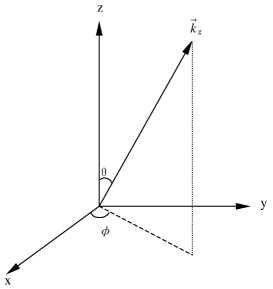
Figure 1: The z-axis is the symmetrical axis of the Gaussian beam, $\vec{k}_{g}$ represents the instantaneous propagating direction of the arbitrary component of the relic GW.

In the following we shall consider the EM resonant response ($\omega_{e}=\omega_{g})$ in different cases. In figure 1 we draw the symmetrical axis (the $z$-axis) of the Gaussian beam and the propagating directions $\vec{k}_{g}$ of the arbitrary component of the relic GWs.

$(a)\ \theta=0$, i.e., the relic GW component propagates along the positive direction of the z-axis.

In this case, as we have shown [10] that the average value of the $x$-component of the first-order perturbative photon flux (PPF) density is

$$n_{x}^{(1)} = -\frac{1}{{\hbar\omega_{e}}}\cdot\left\{{\frac{{A_{\otimes}\hat{B}_{y}^{(0)}\psi_{0}k_{g}y(z+l_{1})}}{{4\mu_{0}\left[{1+(z/f)^{2}}\right]^{1/2}(z+f^{2}/z)}}}\sin\left({\frac{{k_{g}r^{2}}}{{2R}}-\tan^{-1}\frac{z}{f}}\right)\right.$$ (5)

$$+ \frac{{A_{\otimes}\hat{B}_{y}^{(0)}\psi_{0}y(z+l_{1})}}{{2\mu_{0}W_{0}^{2}\left[{1+(z/f)^{2}}\right]^{3/2}}}\left.{\cos\left({\frac{k_{g}r^{2}}{2R}-\tan^{-1}\frac{z}{f}}\right)}\right\}\cdot\exp\left({-\frac{r^{2}}{W^{2}}}\right)$$

$$- \frac{1}{\hbar\omega_{e}}\left\{{\left({1-\frac{4x^{2}}{W^{2}}}\right)\frac{A_{\otimes}\hat{B}_{y}^{(0)}\psi_{0}k_{g}(z+l_{1})}{4\mu_{0}R\left[{1+(z/f)^{2}}\right]^{1/2}}}\right.\cdot\left[{F_{1}(y)\sin\left({\frac{k_{g}x^{2}}{2R}-\tan^{-1}\frac{z}{f}}\right)}\right.$$

$$+ \left.{F_{2}(y)\cos\left({\frac{{k_{g}x^{2}}}{{2R}}-\tan^{-1}\frac{z}{f}}\right)}\right]+\left[{\frac{2}{{W^{2}}}+\left({\frac{{k_{g}^{2}}}{{R^{2}}}-\frac{1}{{W^{4}}}}\right)x^{2}}\right]$$

$$\cdot\frac{{A_{\otimes}\hat{B}_{y}^{(0)}\psi_{0}(z+l_{1})}}{{4\mu_{0}\left[{1+(z/f)^{2}}\right]^{1/2}}}\left[{F_{1}(y)\cos\left({\frac{{k_{g}x^{2}}}{{2R}}-\tan^{-1}\frac{z}{f}}\right)}\right.$$

$$- F_{2}(y)\left.\left.{{\sin\left({\frac{k_{g}x^{2}}{2R}-\tan^{-1}\frac{z}{f}}\right)}}\right]\right\}\exp\left({-\frac{x^{2}}{W^{2}}}\right),(l_{1}\leq z\leq l_{2})$$

where

$$F_{1}(y)=\int{\exp(-\frac{y^{2}}{W^{2}})\cos(\frac{k_{g}y^{2}}{2R})dy,}$$

$$F_{2}(y)=\int{\exp(-\frac{y^{2}}{W^{2}})\sin(\frac{k_{g}y^{2}}{2R})dy,}$$ (6)

are the quasi-probability integrals,$A_{\otimes}=A/a(t)$ is the stochastic value of the amplitude of the relic GW in the laboratory frame of reference, $\hat{B}_{y}^{(0)}$ is the background static magnetic field, which is localized in the region $-l_{1}\leq z\leq l_{2}$, $\psi_{0}$ is the amplitude of electric field of the Gaussian beam, $W_{0}$ is its minimum spot radius, $f=\pi W_{0}^{2}/\lambda_{e}$, $W=W_{0}\left[{1+(z/f)^{2}}\right]^{1/2}$, and $R=z+f^{2}/z$ is the curvature radius of the wavefronts of the Gaussian beam at $z$ (see. e.g., Ref. [16]). We will show that the PPF expressed by Eq. (5) has best perturbative effect than that generated by the relic GW components propagating along other directions.

$(b)\ \theta=\pi$, i.e., the relic GW component propagates along the negative direction of the z-axis.

By using the similar means, one finds

$$n_{x}^{(1)} = -\frac{1}{{\hbar\omega_{e}}}\cdot\left\{{\frac{{A_{\otimes}\hat{B}_{y}^{(0)}\psi_{0}k_{g}y(l_{2}-z)}}{{4\mu_{0}\left[{1+(z/f)^{2}}\right]^{1/2}(z+f^{2}/z)}}}\sin\left({2kz+\frac{{k_{g}r^{2}}}{{2R}}-\tan^{-1}\frac{z}{f}}\right)\right.$$ (7)

$$+ \frac{{A_{\otimes}\hat{B}_{y}^{(0)}\psi_{0}y(l_{2}-z)}}{{2\mu_{0}W_{0}^{2}\left[{1+(z/f)^{2}}\right]^{3/2}}}\left.{\cos\left({2kz+\frac{k_{g}r^{2}}{2R}-\tan^{-1}\frac{z}{f}}\right)}\right\}\cdot\exp\left({-\frac{r^{2}}{W^{2}}}\right)$$

$$- \frac{1}{\hbar\omega_{e}}\left\{{\left({1-\frac{4x^{2}}{W^{2}}}\right)\frac{A_{\otimes}\hat{B}_{y}^{(0)}\psi_{0}k_{g}(l_{2}-z)}{4\mu_{0}R\left[{1+(z/f)^{2}}\right]^{1/2}}}\right.\cdot\left[{F_{1}(y)\sin\left({2kz+\frac{k_{g}x^{2}}{2R}-\tan^{-1}\frac{z}{f}}\right)}\right.$$

$$+ \left.{F_{2}(y)\cos\left({2kz+\frac{{k_{g}x^{2}}}{{2R}}-\tan^{-1}\frac{z}{f}}\right)}\right]+\left[{\frac{2}{{W^{2}}}+\left({\frac{{k_{g}^{2}}}{{R^{2}}}-\frac{1}{{W^{4}}}}\right)x^{2}}\right]$$

$$\cdot\frac{{A_{\otimes}\hat{B}_{y}^{(0)}\psi_{0}(l_{2}-z)}}{{4\mu_{0}\left[{1+(z/f)^{2}}\right]^{1/2}}}\left[{F_{1}(y)\cos\left({2kz+\frac{{k_{g}x^{2}}}{{2R}}-\tan^{-1}\frac{z}{f}}\right)}\right.$$

$$- F_{2}(y)\left.\left.{{\sin\left({2kz+\frac{k_{g}x^{2}}{2R}-\tan^{-1}\frac{z}{f}}\right)}}\right]\right\}\exp\left({-\frac{x^{2}}{W^{2}}}\right),(l_{1}\leq z\leq l_{2})$$

Different from Eq. (5), each and all items in Eq. (7) contain oscillating factor $2kz$. We emphasize that $2kz\approx 419z$ for the high-frequency relic GW of $\nu_{g}=10^{10}\texttt{Hz}$, namely, the factor $2kz$ will play major role in the region of the effective coherent resonance. In other words, the sign of $n_{x}^{(\ref{eq1})}$ will be quickly oscillated and quasi-periodically changed as the coordinate $z$ in the region. Thus the total effective PPF passing through a certain “typical receiving surface” will be much less than that generated by the relic GW component propagating along the positive direction of the $z$-axis, (see Eq. (5) and Table 1)

$(c)\ \theta=\pi/2,\mbox{ }\phi\mbox{ = 0}$ , i.e., the propagating direction of the relic GW component is not only perpendicular to the symmetrical axis of the Gaussian beam, but also vertical to the static magnetic field $\hat{B}_{y}^{(0)}.$

Here we assume that the dimension of the $x$-direction of $\hat{B}_{y}^{(0)}$ is localized in the region $-l_{3}\leq x\leq l_{4}$. Utilizing the similar means, the first-order perturbative EM fields generated by the direct interaction of the relic GW with the static magnetic field can be given by [11]

$$\tilde{E}_{y}^{(\ref{eq1})} = \frac{i}{2}A_{\oplus}\hat{B}_{y}^{(0)}k_{g}c(x+l_{3})\exp[i(k_{g}x-\omega_{g}t)]+\frac{1}{4}A_{\oplus}\hat{B}_{y}^{(0)}c\exp[i(k_{g}x+\omega_{g}t)],$$

$$\tilde{B}_{z}^{(\ref{eq1})} = \frac{i}{2}A_{\oplus}\hat{B}_{y}^{(0)}k_{g}(x+l_{3})\exp[i(k_{g}x-\omega_{g}t)]-\frac{1}{4}A_{\oplus}\hat{B}_{y}^{(0)}\exp[i(k_{g}x+\omega_{g}t)],$$

$$\tilde{E}_{z}^{(\ref{eq1})} = -\frac{1}{2}A_{\otimes}\hat{B}_{y}^{(0)}k_{g}c(x+l_{3})\exp[i(k_{g}x-\omega_{g}t)]+\frac{i}{4}A_{\otimes}\hat{B}_{y}^{(0)}c\exp[i(k_{g}x+\omega_{g}t)],$$

$$\tilde{B}_{y}^{(\ref{eq1})} = \frac{1}{2}A_{\otimes}\hat{B}_{y}^{(0)}k_{g}(x+l_{3})\exp[i(k_{g}x-\omega_{g}t)]+\frac{i}{4}A_{\otimes}\hat{B}_{y}^{(0)}\exp[i(k_{g}x+\omega_{g}t)],$$

$$(l_{3}\leq x\leq l_{4})$$ (8)

In this case the coherent syncro-resonance ($\omega_{e}=\omega_{g})$ between the perturbative fields, Eq. (8), and the Gaussian beam can be expressed as the following first-order PPF density, i.e.,

$$n_{x}^{(\ref{eq1})}=\frac{1}{\mu_{0}\hbar\omega_{e}}\left[{\langle\tilde{E}_{y}^{(\ref{eq1})}\tilde{B}_{z}^{(0)}\rangle+\langle\tilde{E}_{y}^{(0)}\tilde{B}_{z}^{(\ref{eq1})}\rangle-\langle\tilde{E}_{z}^{(\ref{eq1})}\tilde{B}_{y}^{(0)}\rangle}\right],$$ (9)

where $\tilde{B}_{y}^{(0)}$, $\tilde{B}_{z}^{(0)}$ are the $y$- and $z$- components of the magnetic filed of the Gaussian beam, respectively, the angular brackets denote the average over time. Notice that we choose the Gaussian beam of the transverse electric modes (TE), so $\tilde{E}_{z}^{(0)}=0$. By using the same method, we can calculate $n_{x}^{(\ref{eq1})}$, Eq. (9). For example, first term in Eq. (9) can be written as

$$\frac{1}{\mu\hbar\omega_{e}}\langle\tilde{E}_{y}^{(1)}\tilde{B}_{z}^{(0)}\rangle=$$ (10)

$$- \frac{1}{\hbar\omega_{e}}\left\{{\frac{{A_{\oplus}\hat{B}_{y}^{(0)}\psi_{0}k_{g}y(z+l_{3})}}{{4\mu_{0}\left[{1+(z/f)^{2}}\right]^{1/2}(z+f^{2}/z)}}}\sin\left({k_{g}(x-z)+\frac{{k_{g}r^{2}}}{{2R}}-\tan^{-1}\frac{z}{f}}\right)\right.$$

$$+ \frac{{A_{\oplus}\hat{B}_{y}^{(0)}\psi_{0}y(z+l_{3})}}{{2\mu_{0}W_{0}^{2}\left[{1+(z/f)^{2}}\right]^{3/2}}}\left.{\cos\left({k_{g}(x-z)+\frac{k_{g}r^{2}}{2R}-\tan^{-1}\frac{z}{f}}\right)}\right\}\exp\left({-\frac{r^{2}}{W^{2}}}\right)$$

$$- \frac{1}{\hbar\omega_{e}}\left\{{\left({1-\frac{4x^{2}}{W^{2}}}\right)\frac{A_{\oplus}\hat{B}_{y}^{(0)}\psi_{0}k_{g}y(z+l_{3})}{4\mu_{0}R\left[{1+(z/f)^{2}}\right]^{1/2}}}\right.\cdot\left[{F_{1}(y)\sin\left({k_{g}(x-z)+\frac{k_{g}x^{2}}{2R}-\tan^{-1}\frac{z}{f}}\right)}\right.$$

$$+ \left.{F_{2}(y)\cos\left({k_{g}(x-z)+\frac{{k_{g}x^{2}}}{{2R}}-\tan^{-1}\frac{z}{f}}\right)}\right]+\left[{\frac{2}{{W^{2}}}+\left({\frac{{k_{g}^{2}}}{{R^{2}}}-\frac{1}{{W^{4}}}}\right)x^{2}}\right]$$

$$\frac{{A_{\oplus}\hat{B}_{y}^{(0)}\psi_{0}y(z+l_{3})}}{{4\mu_{0}\left[{1+(z/f)^{2}}\right]^{1/2}}}\left[{F_{1}(y)\cos\left({k_{g}(x-z)+\frac{{k_{g}x^{2}}}{{2R}}-\tan^{-1}\frac{z}{f}}\right)}\right.$$

$$- F_{2}(y)\left.\left.{{\sin\left({k_{g}(x-z)+\frac{k_{g}x^{2}}{2R}-\tan^{-1}\frac{z}{f}}\right)}}\right]\right\}\exp\left({-\frac{x^{2}}{W^{2}}}\right),(l_{3}\leq z\leq l_{4}).$$

It can be shown that calculation for the 2nd and 3rd terms in Eq. (9) is quite similar to first term, and they have the same orders of magnitude, we shall not repeat it here. Eq. (8) shows that the $n_{x}^{(\ref{eq1})}$ have a space accumulation effect ($n_{x}^{(\ref{eq1})}\propto x)$. This is because the GWs (gravitons) and EM waves (photons) have the same propagating velocity, so that the two waves can generate an optimum coherent effect in the propagating direction. However, unlike $n_{x}^{(\ref{eq1})}$ produced by the relic GW component propagating along the positive direction of the $z$-axis [see, Eq. (5)], the phase functions in Eq. (10) contain oscillating factor $k_{g}(x-z)$, and it is always possible to choose $l_{1}+l_{2}\gg l_{3}+l_{4}$, i.e., the dimension of the $z$-direction of $\hat{B}_{y}^{(0)}$ is much larger than its $x$-direction dimension. Because of such reasons, the PPF expressed by Eq. (10) will be much less than that repressed by Eq. (5) (see, Table 1).

$(d)\ \theta=\pi/2,\mbox{ }\phi=\pi/2$, i.e., the relic GW component propagates along the y-axis, which is parallel with the static magnetic field $\hat{B}_{y}^{(0)}.$

According to the Einstein-Maxwell equations of the weak fields, then the perturbation of the GW to the static magnetic field vanishes [17], i.e.,

$$n_{x}^{(\ref{eq1})}=0.$$ (11)

It is very interesting to compare $n_{x}^{(\ref{eq1})}$ in Eqs. (5), (7), (10) and (11). As is shown that although they all represent the PPFs propagating along the $x$-axis, their physical behaviors are quite different. In the case of $\theta=\phi=\pi/2$, $n_{x}^{(\ref{eq1})}=0$, Eq. (11); when $\theta=\pi$ and $\theta=\pi/2,\mbox{ }\phi=0$, the PPFs contain the oscillating factors $2k_{g}z$ and $k_{g}(x-z)$, respectively [see Eqs. (7) and (10)]. Only under the condition $\theta=0$, the PPF, Eq. (5), does not contain any oscillating factor, but only slow enough variation function in the z direction. This means that $n_{x}^{(\ref{eq1})}$ produced by the relic GW component propagating along the positive direction of the z-axis, has the best space accumulation effect. Thus our EM system would be very sensitive to the propagating directions of the relic GWs. In other words the EM system has a strong selection capability to the resonant components from the stochastic relic GW background.

The total PPF passing through a certain “typical receiving surface” at the yz-plan will be

$$N_{x}^{(\ref{eq1})}=\int\!\!\!\int\limits_{\triangle S}{\left.{n_{x}^{(\ref{eq1})}}\right|_{x=0}}dydz.$$ (12)

In order to compare the PPFs generated by the different components of the relic GWs, we introduce the typical laboratorial and cosmological parameters:

(1). $\Omega_{gw}\sim 5\times 10^{-6}$, the peak value of the normalized energy density of the high-frequency relic GW ($\nu_{g}=10^{10}\texttt{Hz})$ in the QIM [1]. Then $h\sim\frac{\nu_{H}}{\nu}(\Omega_{gw})^{1/2}\sim 4.48\times 10^{-31}$ [7], i.e., $A_{\oplus},\mbox{ }A_{\otimes}\sim 4.48\times 10^{-31}$, where $\nu_{H}\approx 2\times 10^{-18}\texttt{Hz}$ is the Hubble frequency.

(2). $P=10\texttt{W}$, The power of the Gaussian beam. In this case $\psi_{0}\approx 1.26\times 10^{3}\texttt{Vm}^{-1}$ for the Gaussian beam of $W_{0}=0.05\texttt{m}$.

(3). $\hat{B}_{y}^{(0)}=3\texttt{T}$, the strength of the background static magnetic field.

(4). $0\leq y\leq W_{0}$, $0\leq z\leq 0.3\texttt{m}$, the integration region $\bigtriangleup S$ (the receiving surface of the PPF) in Eq. (12), i.e., $\bigtriangleup S\approx 10^{-2}\texttt{m}^{2}$.

(5). $z=l_{2}+l_{1}=4\texttt{m}$ and $x=l_{3}+l_{4}=0.2\texttt{m}$, (i.e., $\bigtriangleup z\gg\bigtriangleup x)$ they are the interacting dimensions between the relic GWs and the static magnetic field in the $z$ and $x$ directions, respectively.

From the above parameters and Eqs. (5), (7), (10) and (12), we obtain the values of the PPFs as listed in Table 1.

Table 1 shows that the PPF produced by the relic GW component propagating along the positive direction of the symmetrical axis of the Gaussian beam, has a best resonant effect, i.e., largest perturbation and a good space accumulation effect.

As for the distinction between the PPFs and the background photon fluxes, as we have shown [10-12] that utilizing their very different physical behavior in some local regions, they can be split by the special fractal membranes [13,14], so that, the PPFs, in principle, would be observable.

Finally, it should be pointed out that superposition of the relic GWs stochastic components will cause the fluctuation of the PPFs, even if such “monochromatic components” all satisfy the frequency resonant condition ($\omega_{g}=\omega_{e})$. However, Eqs. (5), (7), (10) and (12) show that the metric fluctuation only causes the change of the instantaneous values of the PPFs and does not influence the “direction resonance”. i.e., it does not influence the selection capability of the EM system to the propagating directions of the relic GWs, and it does not influence average effect over time of the PPFs.

Therefore, the high-frequency relic GWs satisfying the above parameters requirement ($h\sim 10^{-31}$ or larger), frequency resonance ($\nu_{e}=\nu_{g}=10^{10}\texttt{Hz})$ and “direction resonance”, in principle, would be selectable and measurable in seconds. More detailed schemes will be studied elsewhere.

Table 1: The PPFs generated by the resonant relic GW components propagating along the different directions, here $\hat{B}^{(0)}=3\texttt{T}$, $A_{\otimes},\mbox{ }A_{\oplus}\sim 4.48\times 10^{-31}$, $\nu_{g}=10^{10}$Hz

The propagating directions	The PPFs (s${}^{-1})$
$z$	4.42$\times$102
$-z$	1.07
$x$	1.42$\times$10-1
$y$	0

References

• [1] Giovannini M 1999 Phys. Rev. D 60 123511
• [2] Giovannini M 1999 Class. Quantum Grav. 16 2905
• [3] Riazuelo A and Uzan J P 2000 Phys. Rev. D 62 083506
• [4] Copeland E J et al 1998 preprint gr-qc/9803070
• [5] Gasperini M and Veneziano G 2003 Physics Reports 373 1
• [6] Veneziano G 2004 Sci. Am, (Int. Ed.), 290 30
• [7] Kogan G S B and Rudenko V N 2004 (Int. Ed) Class. Quantum Grav. 21 3347
• [8] Chincarini A and Gemme G 2003 First Int. Conf. On High-frequency Gravitational waves (Mclean, VA, The Mitre Corporation) Paper-03-103
• [9] Grishchuk L P 2003 preprint gr-qc/0305051
• [10] Li F Y and Yang N 2004 Chin. Phys. Lett. 20 1917
• [11] Li F Y Tang M X and Shi D P 2003 Phys. Rev. D 67 104008
• [12] Baker R M L and Li F Y 2005 Space Technology and Applications International Forum (Alburquerque, New Mexico, Americal Institute of Physics), Paper-008
• [13] Zhou L et al 2003 Appli. Phys. Lett. 82 1012
• [14] Wen W J et al 2002 Phys. Rev. Lett. 89 223901
• [15] Grishchuk L P and Soloklin M 1991 Phys. Rev. D 43 2566
• [16] Yariv A 1975 Quantum Electronics (New York, Wiley) 109
• [17] Boccaletti D et al 1970 Nuovo Cimento B 70 129
Refer to caption