Phenomenological implications of an alternative Hamiltonian constraint for quantum cosmology

Abstract

In this paper we review a model based on loop quantum cosmology that arises from a symmetry reduction of the self dual Plebanski action. In this formulation the symmetry reduction leads to a very simple Hamiltonian constraint that can be quantized explicitly in the framework of loop quantum cosmology. We investigate the phenomenological implications of this model in the semi-classical regime and compare those with the known results of the standard Loop Quantum Cosmology.

I Introduction

Modern observations indicate that, at least on large scales, the Universe appears to be homogeneous and isotropic. In the framework of General Relativity, such a universe is best described by the Friedmann-Robertson-Walker model, which nowadays is the accepted paradigm of cosmology. While the full (non-homogeneous and non-isotropic) theory has infinite degrees of freedom, cosmological models are characterized by a finite-dimensional phase-space. The latter makes cosmology a fruitful testing arena for existing theories of gravity.

One of the central issues of general relativity is the development of space-time singularities. One famous instance is the occurrence of the initial Big-Bang singularity in cosmological models, which takes place under quite general assumptions. As one approaches the Big-Bang singularity, space-time curvature and energy/mass densities blow up, and any description based on classical notion of space-time fails. One is forced to take quantum effects into account and replace General Relativity by a quantum theory of gravity.

Aside from the initial Big-Bang singularity stands the issue of reconciling modern observations with predictions based on the Friedmann equations. Among others there are the flatness and horizon problems. These have been successfully explained by the mechanism called inflation, by introducing matter in theory in the form of a massive scalar field $\phi$, inflaton, minimally coupled to gravity LL . According to the inflationary paradigm, there has to have been an epoch, when the Universe was undergoing an accelerated expansion; such that the size of the Universe increased by a factor of about $e^{60}$ (60 e-foldings) to agree with observations. The mechanism, proposed in LL , considers so called slow-roll approximation, when the inflaton rolls down its potential hill towards the potential minimum, but, at the same time, remaining far away from the minimum. It is exactly in the vicinity of the minimum of the potential, where the inflation stops. For the simplest choice of a quadratic field potential with an arbitrary mass of the inflaton, one would obtain 60 e-foldings if the slow-roll regime starts of at $\phi\approx 3M_{\rm P}$ and ends when the field is essentially zero. The question as to how the inflaton gets to that value before the slow-roll is left for a quantum theory to answer.

Loop quantum gravity (LQG) is believed to be the most plausible candidate for a theory which would reconcile General Relativity and Quantum Mechanics LQG ; ap . It is a background independent non perturbative approach to the canonical quantization of general relativity. The prime prediction of the theory is the discreteness of geometry at the fundamental level: operators corresponding to geometric quantities such as the area and volume have discrete spectra geometrical_op . Geometry gets quantized and at Planckian scales the smooth notion of space and time ceases to exist.

Loop quantum gravity, restricted to a mini-superspace quantization, is called loop quantum cosmology (LQC) ICGC . The major simplifications due to the symmetry reduction make it possible to address physical questions that still remain open in the full theory. For instance LQC provides means for the understanding and resolution of the Big-Bang singularity. The important physical question of whether classical singularities of general relativity are absent in the quantum theory is answered in the affirmative in LQC Bojowald:2001xe ; ABL ; sing-res (for a recent review see ICGC ). This remarkable result originates from the fundamental discreteness of geometric operators, which dramatically changes the quantum ‘evolution’ equation in the deep Planckian regime. It has also been shown that LQC leads to modifications of the classical Friedmann equations ModFried ; 2ndCorr . Recent works have shown that these effects can provide the proper initial conditions for chaotic inflation Ambiguities ; ChaInf ; closedinflation and may lead to measurable effects on the CMB CMB .

LQC studies the quantum evolution of a homogeneous and isotropic universe. One starts from the symmetric Einstein-Hilbert action and performs the Legendre transform to obtain the Hamiltonian constraint. The wave function of the universe is to be annihilated by the quantum counterpart of the constraint. By virtue of the underlying discreteness, the equations governing the evolution in the deep Planckian regime are difference equations rather than differential equations. In other words, as the notion of the infinitesimal translation ceases to exist at this scale, only an operator of a finite translation can be well-defined, thus replacing the common derivation operator.

It is, however, sensible to expect that at some scale, $a_{0}$, the space-time would become essentially smooth and continuous. Indeed, it was shown in Semi ; Semi_SV that in the continuum limit the difference equation yields the well-known Wheeler-deWitt equation, which is an indication in favour of the viability of LQC. On the other hand, it would make sense to suppose that there exist an intermediate range of scale factors, $a_{0}\lesssim a\lesssim a_{*}$, for which the space time is not yet classical, i.e. the non-perturbative modifications play a substantial role. This approximation is called semi-classical.

To make the notion of semi-classicality more precise, we should specify the upper and lower bounds of the scale factor. In Semi ; Semi_SV shown that the difference equations are well approximated by Friedmann differential equations for scale factors above $a_{0}\approx\sqrt{\gamma\mu_{0}}l_{\rm P}$ ($\mu_{0}\equiv\sqrt{3}/4$ being quantum ambiguity parameter related to the lowest eigenvalue of the area operator in LQG ABL ). Here $l_{\rm P}=\sqrt{G\hbar}$ is the Planck length and $\gamma\approx 0.2375$ is the Barbero-Immirzi parameter, controlling discreteness of the quantum space-time, whose value is determined from black hole thermodynamics bek_hawking1 . For a minimally coupled scalar field, the quantum corrections manifest themselves via the geometrical density (inverse volume) operator. The crucial result of LQC is that the spectrum of this operator turns out to be bounded from above (classically it blows up) as $a\rightarrow 0$. Moreover, for small scale factors it becomes proportional to a positive power of $a$. The classical behaviour of the geometrical density operator is recovered soon after $a\geq a_{*}\equiv\sqrt{\gamma\mu_{0}j/3}l_{\rm P}$ ($j$ being a half-integer, greater that unity), thus defining the upper bound of the semi-classical regime.

One of the open issues of LQG that remains is the characterization of the physical Hilbert space, which needs a physical inner product and a notion of unitary evolution. That, in turn, requires one to construct a self-adjoint Hamiltonian constraint operator. As the standard Hamiltonian obtained from the Einstein-Hilbert action is not self-adjoint, one has to symmetrize it in a non-trivial way Semi ; Willis . An alternative way, usually taken by Spin Foams theorists, is based on the Plebanski action pleb , which classically is equivalent to the Einstein-Hilbert action. In this formulation the symmetry reduction leads to a very simple Hamiltonian constraint that is self-adjoint and can be quantized explicitly in the framework of LQC NPV . The model is defined in the Riemannian sector, which constitutes a limitation when considering physical predictions. However, a method for transforming to the Lorentzian sector was shown in Ref. NPV , and it was argued that the main results of the model hold true in the Lorentzian sector.

In this paper we review a model based on LQC that arises from a symmetry reduction of the self-dual Plebanski action. We show that in the homogeneous and isotropic case, the Plebanski action can be viewed as the standard one (symmetry reduced Einstein-Hilbert action) with a specific choice of the lapse function. As far as the lapse plays the role of a Lagrange multiplier imposing the Hamiltonian constraint, both actions must agree classically and yield the same physics. Upon quantization, however, the arbitrariness of lapse gives rise to yet one more (lapse) ambiguity. We must, nevertheless, emphasize that the two actions cannot be related merely by a choice of lapse in the full theory, the correspondence holds only for the symmetry-reduced models. Therefore, from now on we will avoid using the word ‘ambiguity’, as it is commonly referred to in the context of the full theory. Various quantization ambiguities present in LQC are discussed in great detail in Ambiguities . In current paper we deliberately leave out all ambiguities (except for the parameter $j$) and focus on the lapse arbitrariness. (In particular, we fix the parameter $l$ appearing in the geometrical density operator (see Ambiguities ) at its natural value $l=3/4$.)

While this specific choice of lapse appears automatically, when obtained as the result of the classical symmetry reduction of the full theory, its explicit form is, indeed, natural, as it leads to a self-adjoint Hamiltonian constraint.

Generally, such a lapse arbitrariness would lead to different quantum theories in both deep Planckian regime and semi-classical regime. We are focusing on the semi-classical approximation. The goal of this work is to investigate the robustness of the theory with respect to this kind of ‘ambiguity’. We show that the quantum-corrected Friedmann equations indeed lead to (semi-classical) inflation, which provides conditions for the classical slow-roll regime. Also, the solutions for both standard and Plebanski models may differ substantially during the semiclassical inflation, but get very close to each other in the classical domain. Moreover, for observationally interesting solutions (those corresponding to the maximum value of the inflaton of about $3{\rm M}_{P}$) the difference between the two models is insignificant even within the domain of the semi-classical approximation.

II Classical Theory

In this section we illustrate the basic ideas underlying LQC. Conventionally, one starts with the Einstein-Hilbert action of General relativity and performs its symmetry reduction, assuming isotropy and homogeneity. The simplified action, written in the Hamiltonian formulation, is subject to the standard Dirac quantization. It turns out that the Hamiltonian of the system is weakly zero, and the dynamics is governed by the (Hamiltonian) constraint.

Firstly, we review the standard method used to obtain the Hamiltonian constraint from the Einstein-Hilbert action in the framework of the FRW model and derive Friedmann’s equations. Secondly, in section (II.1) we consider an alternative formulation of the gravitational action, which yields equivalent classical equations of motion, but proves to be different upon quantization.

II.1 Standard formulation

The Einstein-Hilbert action is given by

$$S_{EH}=\frac{1}{2\kappa}\int d^{4}x\sqrt{|g|}R,\qquad\qquad(\kappa=8\pi G)$$ (1)

($g$ being the determinant of the metric and $R$ the Ricci scalar) and consider a general flat and isotropic model

$$g_{ab}dx^{a}dx^{b}=-N^{2}dt^{2}+a^{2}d{\vec{x}}^{2}$$ (2)

Here $N$ is the lapse function and $a$ is the scale factor. Calculating the scalar curvature as usual, and inserting into (1), we obtain

$$S_{EH,\rm iso}=\frac{1}{2\kappa}\int\frac{dt}{N}\left[6a^{2}\ddot{a}+6a\dot{a}^{2}\right]$$ (3)

We then proceed to introduce the connection $A_{a}^{i}$ and densitized triad $\tilde{E}_{i}^{a}$ variables as follows:

$$\tilde{E}_{i}^{a}\tilde{E}_{i}^{b} = |q|q^{ab}$$ (4)

$$A_{a}^{i} = \Gamma_{a}^{i}+\gamma K^{i}_{a}$$ (5)

where $q_{ab}$ represents the spatial metric, $\Gamma_{a}^{i}$ the intrinsic curvature, $K_{a}^{i}$ the extrinsic curvature and $\gamma$ the Barbero-Immirzi parameter. Due to flatness and isotropy, these quantities can be expressed in terms of two (time-dependent) numbers as follows:

$$\tilde{E}_{i}^{a}=c\delta_{i}^{a},\qquad A_{a}^{i}=p\delta_{a}^{i}$$ (6)

Using the definitions (4) and (5) and the fact that in a flat isotropic spacetime we have:

$$\Gamma_{a}^{i}=0,\qquad K_{a}^{i}=\frac{\dot{a}}{N}\delta_{a}^{i}$$ (7)

we obtain an expression for $p$ and $c$ in terms of $a$, $\dot{a}$:

$$p=a^{2},\qquad c=\gamma\frac{\dot{a}}{N}$$ (8)

from which:

$$S_{LQC}=\frac{3}{\kappa}\int dt\left[\frac{p\dot{c}}{\gamma}+N\frac{\sqrt{p}c^{2}}{\gamma^{2}}\right]$$ (9)

Note that one can, of course, arrive at the same expression inserting $A_{a}^{i}$ and $\tilde{E}_{i}^{a}$ of (6) into the action of the full theory ABL :

$$H_{\rm gr} := \int d^{3}xN\,e^{-1}\left(\epsilon_{ijk}F_{ab}^{i}\tilde{E}^{aj}\tilde{E}^{bk}\right.$$ (10)

$$- 2(1+\gamma^{2})K_{[a}^{i}K_{b]}^{j}\tilde{E}_{i}^{a}\tilde{E}_{j}^{b}\left.\right)$$

$$= -\gamma^{-2}\int d^{3}x\,N\,\epsilon_{ijk}F_{ab}^{i}\,\,e^{-1}{\tilde{E}^{aj}\tilde{E}^{bk}}$$

where $e:=\sqrt{|\det E|}\,\,\text{sgn}(\det E)$, $F_{ab}^{i}$ is the curvature of the connection. In the second step we have used the fact that for spatially flat, homogeneous models the two terms in the full constraint are proportional to each other. Technically the integral diverges, since the left invariant metric is constant and the integral is over a non compact manifold. To overcome this, we restrict the integral to a finite cell with volume $V_{0}$ and absorb this factor into the variables as $A_{a}^{i}\,(p)\rightarrow V_{0}^{2/3}A_{a}^{i}\,(p)$ and $\tilde{E}_{i}^{a}\,(c)\rightarrow V_{0}^{1/3}\tilde{E}_{i}^{a}\,(c)$. By doing so, one obtains the action (9).

The action (9) is expressed in terms of the canonical variable $c$ and its conjugate momentum $p^{\prime}=3p/\kappa\gamma$. This yields the Poisson brackets:

$$\{c,p\}=\frac{\kappa\gamma}{3}.$$ (11)

Because of homogeneity, the lapse $N$ can depend only on time and plays the role of a Lagrange multiplier: $N$ being freely specifiable, the coefficient of $N$ in the action needs to be identically zero, yielding the Hamiltonian Constraint

$${\cal H}_{\rm gr}\equiv-\frac{3\sqrt{p}c^{2}}{\kappa\gamma^{2}}=0$$ (12)

or, if matter is present in the form of a scalar field $\phi$, with Hamiltonian

$${\cal H}_{\phi}=\frac{p_{\phi}^{2}}{2p^{3/2}}+p^{3/2}V(\phi),$$ (13)

$p_{\phi}$ being the field momentum, then

$${\cal H}=-\frac{3\sqrt{p}c^{2}}{\kappa\gamma^{2}}+{\cal H}_{\phi}=0$$ (14)

The Hamilton equations of motion now follow:

$$\dot{p} = \{p,N{\cal H}\}=-\frac{\gamma\kappa}{3}\frac{\partial{\cal H}}{\partial c}=\frac{2c}{\gamma}\sqrt{p}$$ (15)

$$\dot{c} = \{c,N{\cal H}\}=\frac{\gamma\kappa}{3}\frac{\partial{\cal H}}{\partial p}$$ (16)

$$= \frac{\gamma\kappa}{2}\left(\frac{c^{2}}{2\gamma\sqrt{p}}-\frac{p_{\phi}^{2}}{p^{5/2}}+\sqrt{p}V(\phi)\right)$$

$$\dot{\phi} = \{\phi,N{\cal H}\}=\frac{p_{\phi}}{p^{3/2}}$$ (17)

$$\dot{p}_{\phi} = \{p_{\phi},N{\cal H}\}=-p^{3/2}V_{,\phi}(\phi)$$ (18)

We have also used the lapse freedom and set $N=1$. Note that only three phase variables are independent. For later convenience, we shall eliminate one of them (specifically, the connection $c$) using the Hamiltonian constraint (14). One can easily show that the equations above lead to familiar Friedmann’s equations. The constraint equation, rewritten in terms of the scale factor and its time derivative, reads

$${\cal H}=-\frac{3}{\kappa}a\dot{a}^{2}+\frac{a^{3}}{2}\dot{\phi}^{2}+a^{3}V(\phi)\approx 0$$ (19)

Dividing by $a^{3}$, one gets the first Friedmann equation:

$$H^{2}=\frac{\kappa}{3}\left[\frac{\dot{\phi}^{2}}{2}+V(\phi)\right]$$ (20)

Here $H\equiv\dot{a}/a$ is the Hubble rate. Using the $\dot{p}_{\phi}$-equation we derive the Klein-Gordon equation

$$\ddot{\phi}+3H\dot{\phi}+V,_{\phi}(\phi)=0$$ (21)

Finally, the Raychaudhuri equation can be obtained by taking the time derivative of (20) and substituting $\ddot{\phi}$ from (21):

$$\dot{H}=-\frac{\kappa}{2}\dot{\phi}^{2}$$ (22)

These equations particularly tell us, that for any reasonable scalar field and an expanding universe ($H>0$), (21) looks like an oscillator equation with dissipation, whereas (22) implies decelerated expansion. We shall see that if quantum effects are taken into account, the universe can expand accelerating (super-inflation), and the friction term can become negative, thus driving the scalar field (inflaton) up-hill.

II.2 Plebanski formulation

We start, following NPV , by considering the classical self-dual Riemannian gravitational action, symmetry reduce it to the homogeneous and isotropic model and show that the system would be governed by equations of motions equivalent to the standard ones of the previous section.

As noted by Plebanskipleb the classical self-dual Riemannian gravitational action can be written as

$$S[A,\Sigma,\psi]=\frac{2}{\kappa}\int\Sigma_{i}\wedge F^{i}(A)-\psi_{ij}\left[\Sigma^{i}\wedge\Sigma^{j}-\frac{1}{3}\delta^{ij}\Sigma^{k}\wedge\Sigma_{k}\right]$$ (23)

where $\Sigma=\Sigma^{i}_{\mu\nu}dx^{\mu}dx^{\nu}\tau_{i}$ is an SU(2) Lie algebra valued two form, $A=A^{i}_{\mu}dx^{\mu}\tau_{i}$ is an SU(2) Lie algebra valued connection, $\tau_{i}$ are the generators of the Lie algebra of SU(2). The tensor $\psi_{ij}$ is symmetric and acts as a Lagrange multiplier enforcing the constraint $\Sigma^{i}\wedge\Sigma^{j}-\frac{1}{3}\delta^{ij}\Sigma^{k}\wedge\Sigma_{k}=0$. Once this constraint is solved, the action becomes equivalent to the self-dual action of general relativity. The model is defined in the Riemannian sector which constitutes a limitation when considering physical predictions. However, in NPV was shown a method for transforming to the Lorentzian sector and argued that the main results of the model are manifested in the Lorentzian sector.

In order to reduce the action (23) to spatial homogeneity and isotropy, we write the action explicitly in terms of coordinates separating space and time (which we here call $\tau$ to avoid confusion with the previous section) as

$$S[A,\tilde{E},B] = \frac{2}{\kappa}\int d\tau\int d^{3}\!xA^{i}_{a,\tau}\tilde{E}^{a}_{i}+A^{i}_{0}D_{a}\tilde{E}^{a}_{i}+\epsilon^{abc}B^{i}_{a}F^{i}_{bc}$$ (24)

$$- \psi_{ij}\left[\frac{1}{2}B^{i}_{a}\tilde{E}^{aj}+\frac{1}{2}B^{j}_{a}\tilde{E}^{ai}-\frac{4}{3}\delta^{ij}B^{k}_{a}\tilde{E}^{a}_{k}\right]$$

where we introduced the definitions $\tilde{E}^{ai}(\equiv\sqrt{q}E^{ai})\equiv\,\epsilon^{abc}\Sigma^{i}_{bc}$, $B^{i}_{a}\equiv 2\,\Sigma^{i}_{0a}$, and $\epsilon^{abc}=\epsilon^{0abc}$. Assuming spatial homogeneity and isotropy, we take the triad and connection of the form (6) and, similarly, $B_{a}^{i}=B\delta_{a}^{i}$. Written in terms of the reduced variables the homogeneous and isotropic gravitational action becomes

$$S_{\rm Pleb}[c,p,B] = \frac{3}{\kappa}\int\!\!d\tau\int\!\!d^{3}\!x\;(\sqrt{q}pc_{,\tau}+\sqrt{q}Bc^{2})$$ (25)

$$= V_{0}\frac{3}{\kappa}\int\!\!d\tau\;(pc_{,\tau}+Bc^{2})$$

where $V_{0}\equiv\int\!\!d^{3}\!x\sqrt{q}$. The constraint term $\psi_{ij}\left[B^{i}_{a}\tilde{E}^{aj}+B^{j}_{a}\tilde{E}^{ai}-\frac{1}{3}\delta^{ij}B^{k}_{a}\tilde{E}^{a}_{k}\right]$ in the full action (24) vanishes identically for the isotropic model which can be checked by a direct calculation. Here we again integrate over a finite cell with volume $V_{0}$ and absorb this factor into the variables as $p\rightarrow V_{0}^{2/3}p$, $c\rightarrow V_{0}^{1/3}c$, and $B\rightarrow V_{0}^{1/3}B$, whence the action becomes

$$S_{\rm Pleb}(c,p,B)=\frac{3}{\kappa}\int\!\!d\tau\;(pc_{,\tau}+B\,c^{2}).$$ (26)

Since ${\cal H}_{\rm gr}\approx 0$ (see 12), the action (9) admits time reparametrization. In particular, setting $d\tau$=$\sqrt{p}dt$, one obtains the action above. Taking this into account, one can formally introduce the matter part in the action as:

$${\cal H}_{\rm Pleb}=-\frac{3c^{2}}{\kappa\gamma^{2}}+\frac{1}{\sqrt{p}}{\cal H}_{\phi}$$ (27)

Note that ${\cal H}_{\rm Pleb}$ does not have units of energy while ${\cal H}_{\phi}$ does. Hence we have written the prefactor $\frac{1}{\sqrt{p}}$, such that ${\cal H}_{\phi}$ coincides with the standard form of the matter Hamiltonian (Eq. 13). We conclude the section with Hamilton’s equations of motion

$$p_{\tau}=\{p,B{\cal H}_{\rm Pleb}\}=\frac{2c}{\gamma}$$ (28)

$$c_{\tau}=\{c,B{\cal H}_{\rm Pleb}\}=\frac{2\gamma\kappa}{3}\left(-\frac{p_{\phi}^{2}}{p^{3}}+V(\phi)\right)$$ (29)

$$\phi_{\tau}=\{\phi,B{\cal H}_{\rm Pleb}\}=\frac{p_{\phi}}{p^{2}}$$ (30)

$$p_{\phi,\tau}=\{p_{\phi},B{\cal H}_{\rm Pleb}\}=-pV_{,\phi}(\phi)$$ (31)

Here we similarly set $B=1$ to arrive at the righthand side of the equations of motion. From now on, we shall no longer use the connection, $c$. We will rather express it in terms of the three other phase variables, using Eq. (14)

$$\frac{c}{\gamma}=\sqrt{\frac{\kappa}{3}}\sqrt{pV(\phi)+\frac{p_{\phi}^{2}}{2p^{2}}}$$ (32)

Note that Eq. (27) yields the same result. It is also straightforward to show that the Hamilton equations above reproduce the standard ones, after the backward time reparametrization $d\tau$=$\sqrt{p}dt$. One can also put it the following way. Identify the time variables, $t$ and $\tau$, but think of the two actions, (9) and (26), as described by different lapse functions. Specifically, the former corresponds to $N=1$, whereas the latter is related to $B\equiv\sqrt{p}N=1$. In other words, the two descriptions lead to the same classical equations of motion, if one sets

$$N=1/\sqrt{p}$$ (33)

We shall,however, see that the loop quantization of the two constraints (14) and (27) gives rise to a discrepancy between the two models, and the quantum corrected dynamics shall be different in the semi-classical approximation.

III Quantization

In order to quantize a theory, one promotes mutually conjugate variables to operators, whose commutation relation derives from the Poisson bracket of the classical theory. In the framework of the conventional (Schrödinger) quantization, the operators are defined in a way that one of them acts as a multiplication, while the other one is a derivation. Applied to cosmology this leads to the famous Wheeler-DeWitt equation which provides an accurate description of the wavefunction of the universe at relatively large scales, but fails in describing classical singularities. For at the Planckian scale smooth space-time is no longer a meaningful notion, hence derivative cannot be well-defined. The problem can be solved in the framework of another quantization scheme, which is based on holonomies around closed loops and is called Loop Quantization. The basic idea is that one needs to replace derivatives or, more precisely, differentials (that can be thought of as infinitesimal translations) with (finite) translations respecting the fundamental discreteness of space-time in the deep Planckian regime. In this section we consider the Loop Quantization procedure for the constraints (14) and (27) and then discuss the implications in the semi-classical regime.

III.1 Standard formulation

The lesson taught by the full theory states that if one works in the tetrad representation, the connection cannot be promoted to a well defined operator. Instead one is forced to reformulate the theory in terms of holonomies of the connection, whose operators constitute translations. The main result of the loop quantization, that we would need in this paper, is the spectrum of the geometrical density operator $(\widehat{1/a^{3}})$. If we consider the matter Hamiltonian (13), we see that (classically) the kinetic term apparently blows up as $p$ approaches zero. Moreover, the naive attempt to write the geometrical density operator $(\widehat{1/a^{3}})$ as $\hat{a}^{-3}\equiv\hat{p}^{-3/2}$ fails simply because the triad operator has a zero eigenvalue in its discrete spectrum, hence cannot be inverted. Nonetheless, the inverse scale factor operator can be defined in terms of a commutator of well behaved operators ABL ; closedinflation . Classically we have

$$a^{-3}=\left[\frac{1}{2\pi G\gamma}\left\{c,|p|^{3/4}\right\}\right]^{6}$$ (34)

which after quantization becomes ICGC

$$d_{j}(a)=D(q)\,a^{-3},~{}~{}q:=a^{2}/a_{*}^{2},~{}~{}a_{*}:=\sqrt{j\gamma\mu_{0}/3}\,l_{P}$$ (35)

where

$$D(q) = q^{3/2}\left\{\frac{8}{11}\right.\left[(q+1)^{11/4}-|q-1|^{11/4}\right]$$ (36)

$$- \frac{8}{7}q\left.\left[(q+1)^{7/4}-{\rm sgn}(q-1)|q-1|^{7/4}\right]\right\}^{6}$$

The asymptotic behaviour of the density operator follows from the equation above. Not only does $d_{j}$ remain bounded for $a\rightarrow 0$, it becomes proportional to a positive power of the scale factor. Specifically, $D(q)\propto a^{15}$ and $d\propto a^{12}$, thus making the matter Hamiltonian (13) well behaved. On the other hand, as $a$ goes to infinity, one recovers the classical dependence: $D(q)\approx 1$ whereas $d\approx a^{-3}$.

We have seen that in the deep Planckian regime, when $a\approx a_{0}\equiv\sqrt{\gamma\mu_{0}}l_{P}$, one is forced to use the difference equation. The classical description (20,21,22) works for $a\gg a_{*}$. There is, however, an intermediate range of scale factors Semi_SV , $a_{0}\ll a\ll a_{*}$, when space-time is essentially smooth, so that differential equations can be used, and also quantum corrections are significant, i.e. $D(q)$ behaves non-classically. In that case, one would use the Hamilton equations dictated by the Hamiltonian constraint, modified in the following way. Every negative power of the scale factor should be replaced by the appropriate power of $d_{j}$:

$${\cal H}_{\rm Std}=-\frac{3\sqrt{p}c^{2}}{\kappa\gamma^{2}}+d_{j}\frac{p_{\phi}^{2}}{2}+p^{3/2}V(\phi),$$ (37)

The quantum corrected Friedmann, Klein-Gordon and Raychaudhuri equations would then read:

$$H^{2}=\frac{\kappa}{3}\left(\frac{\dot{\phi}^{2}}{2}D(q)^{-1}+V(\phi)\right)$$ (38)

$$\ddot{\phi}+3H\dot{\phi}\left(1-\frac{\cal D}{3}\right)+D(q)V,_{\phi}(\phi)=0$$ (39)

$$\dot{H}=-\frac{\kappa}{2}D(q)^{-1}\dot{\phi}^{2}\left(1-\frac{\cal D}{6}\right)$$ (40)

where we have introduced the logarithmic derivative

$${\cal D}:=\frac{d{\rm ln}(D)}{d{\rm ln(a)}}\equiv\frac{\dot{D}}{HD}$$ (41)

III.2 Plebanski formulation

Earlier we had pointed out, that one can pass directly to the semi-classical regime starting from the homogeneous and isotropic Hamiltonian constraint of the theory. The recipe was to replace all classical negative powers of the scale factor with the appropriate powers of the eigenvalues of the geometrical density operator, $d_{j}(a)$ (36). The modified constraint becomes

$${\cal H}_{\rm Pleb}=-\frac{3c^{2}}{\kappa\gamma^{2}}+d_{j}^{4/3}\frac{p_{\phi}^{2}}{2}+pV(\phi)$$ (42)

here $c=\gamma aa_{\tau}$ as before, and

$$p_{\phi}=\phi_{,\tau}d_{j}^{4/3}\equiv\phi_{,\tau}D(q)^{-4/3}a^{4}$$ (43)

Note that the major difference between the standard and Plebanski effective theories arises from the $d_{j}^{4/3}$ factor of equation (42). Rewriting the constraint as

$${\cal H}_{\rm Pleb}=-\frac{3}{\kappa}a^{2}a_{,\tau}^{2}+D(q)^{-4/3}a^{4}\frac{\phi_{,\tau}^{2}}{2}+a^{2}V(\phi)=0$$ (44)

we obtain the quantum corrected Friedmann, Klein-Gordon and Raychaudhuri equations:

$$\tilde{H}^{2}=\frac{\kappa}{3}\left(\frac{\phi_{,\tau}^{2}}{2}D(q)^{-4/3}+\frac{V(\phi)}{a^{2}}\right)$$ (45)

$$\phi_{,\tau\tau}+4\tilde{H}\phi_{,\tau}\left(1-\frac{\cal D}{3}\right)+\frac{D(q)^{4/3}}{a^{2}}V,_{\phi}(\phi)=0$$ (46)

$$\tilde{H}_{,\tau}=-\frac{\kappa V(\phi)}{3a^{2}}-\frac{2\kappa}{3}D(q)^{-4/3}\phi_{,\tau}^{2}\left(1-\frac{\cal D}{6}\right)$$ (47)

note that the logarithmic derivative $\cal D$ defined in (41) is lapse independent, hence we keep the same notation. Also, performing a direct calculation, one can show that under $\tau\rightarrow t$ the equations above become very similar to the ones of the previous section (38, 39, 40), up to the replacement $D\rightarrow D^{4/3}$ (and hence ${\cal D}\rightarrow 4{\cal D}/3$). Obviously, in the classical limit: $D\approx 1$, ${\cal D}\approx 0$, hence the two sets of equations coincide.

For numerical purposes, however, it is more convenient to use the (quantum corrected) Hamilton equations of motion. As far as the connection variable $c$ has been eliminated, they become a system of three first order ordinary differential equations and thus can be solved by standard means. We now restrict ourselves to the quadratic field potential

$$V(\phi)=\frac{1}{2}m_{\phi}^{2}\phi^{2}$$ (48)

and write out the modified equations

$$\dot{p}=\sqrt{\frac{16\pi}{3}}\sqrt{p^{2}\phi^{2}+D\left(\frac{p}{\alpha}\right)^{4/3}\frac{p_{\phi}^{2}}{p}}$$ (49)

$$\dot{\phi}=D\left(\frac{p}{\alpha}\right)^{4/3}\frac{p_{\phi}}{p^{3/2}}$$ (50)

$$\dot{p}_{\phi}=-p^{3/2}\phi$$ (51)

where $\alpha\equiv\gamma j/3$, and the phase variables have been written in the following units:

$$[p]=l_{\rm P}^{2},\,[\phi]=l_{\rm P}^{-1}\equiv M_{\rm P},\,[t]=m_{\phi}^{-1},\,[p_{\phi}]=m_{\phi}l_{\rm P}^{2}$$ (52)

Note, again, that the Hamilton equations for the standard LQC can be recovered from the corresponding Plebanski ones by replacing all the exponents (4/3) of $D(p/\alpha)$ with a unity. In the following section we present some solutions for the equations above for the both models and analyze how they compare with one another.

IV Phenomenological Implications

In this section we introduce some typical solutions to the Hamilton equations of motion. The key question is how one chooses initial conditions. While the choice for $p_{i}\equiv a_{0}^{2}=\gamma\mu_{0}(l_{\rm P}^{2})$ seems rather obvious, the initial values of the inflaton, $\phi_{i}$, and its conjugate momentum, $p_{\phi}$, is a more subtle issue Ambiguities . Consider the inflaton as a wavepacket, localized around $\{\bar{\phi},\bar{p}_{\phi}\}$, with a spread {$\Delta\phi,\Delta p_{\phi}$} constrained by the uncertainty principle (written in the Planck units)

$$\Delta\phi\,\Delta p_{\phi}\geq 1$$ (53)

We are interested in the inflaton starting off near the potential minimum. As the uncertainty principle does not restrict the expectation values of the wavepacket, one can consistently specify the initial values to be $\bar{\phi}=0=\bar{p}_{\phi}$. Then, from the probabilistic point of view, the most likely values for the inflaton are of order of the spreads $\Delta\phi$ and $\Delta p_{\phi}$. Obviously the initial value $\phi_{i}$ should be much less than $3M_{\rm P}$. Therefore we set $\phi_{i}=0.1(M_{\rm P})$, and $p_{\phi i}\equiv 1/\phi_{i}=10(l_{\rm P})$. Note that had we chosen a lower $\phi_{i}$, that would have led to a higher initial momentum, thus making successful inflation more likely.

Let us now compare the initial energy of the inflaton field in the Plebanski and standard models

$${\cal H}_{\rm Pleb}^{(\phi)} = D(q)^{4/3}\frac{p_{\phi}^{2}}{2p^{3/2}}+p^{3/2}V(\phi)$$

$${\cal H}_{\rm Std}^{(\phi)} = D(q)\frac{p_{\phi}^{2}}{2p^{3/2}}+p^{3/2}V(\phi)$$ (54)

Provided the same initial conditions for both models, compare the corresponding values of the initial energy. Since $D(q)<1$ for $a_{0}\ll a_{*}$, we conclude that

$$H_{\rm Pleb}^{(\phi)}<H_{\rm Std}^{(\phi)}$$

The latter implies a lower inflation for the Plebanski model.

The three graphs below depict the time dependence of the the scalar field, $\phi(t)$ (Fig. 1-3), and the scale factor, $a(t)$ (Fig. 4-6), for different values of the parameter $j$. Specifically we chose $j~{}=~{}100,10$ and 5. The qualitative dynamics for all the figures can be described as follows. Initially: $a\ll a_{*},\,D(q)\ll~{}1,\,{\cal D}>~{}6$. Thus the right hand side of the Raychaudhuri equations (40 ,47) is positive (for the potential term in (47) can be neglected), the inflaton goes up the potential hill driving super-inflation ($\dot{H}>0$). When ${\cal D}\approx 6$, the right hand side of (40) and (47) becomes negative thus ending the super-inflationary phase. The scalar field proceeds up-hill until ${\cal D}\approx 3$, turning into the slow-roll regime with the oscillatory behaviour.

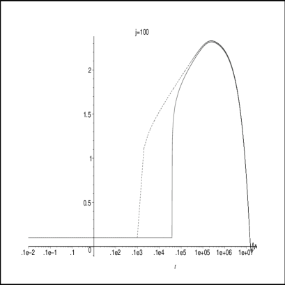
Figure 1: Time dependence of the inflaton field for $j~{}=~{}100$. Dashed and solid curves correspond to the standard and Plebanski models respectively

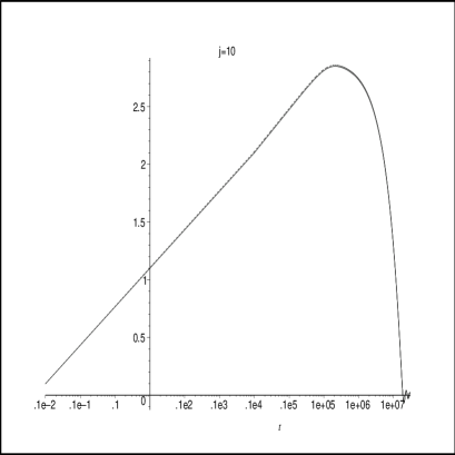
Figure 2: Time dependence of the inflaton field for $j~{}=~{}10$. Dashed and solid curves correspond to the standard and Plebanski models respectively

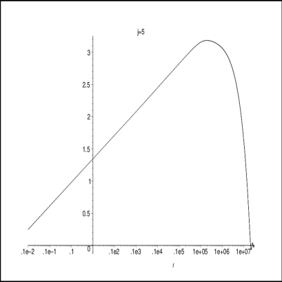
Figure 3: Time dependence of the inflaton field for $j~{}=~{}5$. Dashed and solid curves correspond to the standard and Plebanski models respectively

As the first three figures suggest, the maximum magnitude of the inflaton, $\phi_{max}$, becomes greater for smaller $j$s. Further numerical analysis shows that $\phi_{max}$ exceeds the required value of 3M_P at $j\approx 5$. As was expected the Plebanski model gives a bit lower inflation.

We also see that in the semi-classical regime the evolution of the inflaton of the Plebanski action differs from that of the standard one. The difference is more significant for larger $j$s. Note, however, that as $j$ decreases the discrepancy between the curves describing the scalar field for the two models becomes more and more negligible. In order to analyze this feature, let us first rescale the variables $p$ and $p_{\phi}$. Choosing the units for the scale factor to be $a_{*}\equiv\sqrt{\alpha}l_{\rm P}$ instead of $l_{\rm P}$, along with $[p_{\phi}]\rightarrow[p_{\phi}]\alpha^{3/2}$, we can completely get rid of $j$ in the equations of motion. It now appears in the initial conditions bringing modifications into the uncertainty principle (53)

$$\Delta\phi\,\Delta p_{\phi}=\alpha^{3/2}$$

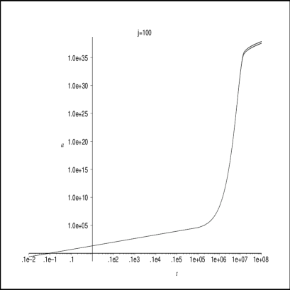
Figure 4: Time dependence of the scale factor for $j~{}=~{}100$. Dashed and solid curves correspond to the standard and Plebanski models respectively

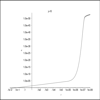
Figure 5: Time dependence of the scale factor for $j~{}=~{}10$. Dashed and solid curves correspond to the standard and Plebanski models respectively

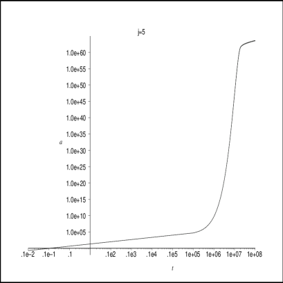
Figure 6: Time dependence of the scale factor for $j~{}=~{}5$. Dashed and solid curves correspond to the standard and Plebanski models respectively

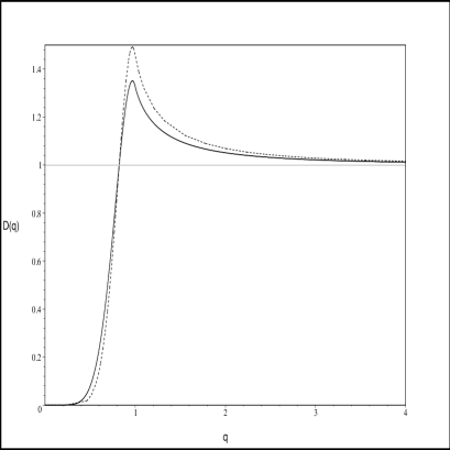
Figure 7: Spectrum of the geometrical density operator $D(q)$ (solid curve) compared to $D(q)^{4/3}$ (dashed curve)

Nonetheless, the initial conditions for both models still coincide, and the only difference between the two sets of equations of motion is the exponent of the geometrical density spectrum. In the graph below we plot the dependencies of $D(q)$ and $D(q)^{4/3}$ (Fig. 7). With the units chosen above, $a=a_{*}$ corresponds to $q=1$.

Let us now consider the logarithmic derivative, $\cal D$. From the quantum corrected Friedmann equations we see that at ${\cal D}=6$ the phase of superinflation ends, whereas at ${\cal D}=3$ the anti-friction term of the Klein-Gordon equation turns into normal friction. These values of the logarithmic derivative occur at $q=0.91$ and $q=0.84$ respectively. Emphasize that they are the same for both models and are in the range, where $D(q)\approx 1$ thus the difference between $D$ and $D^{4/3}$ in Fig. 7 is small.

With the choice of units above, the initial value of the scale factor is

$$a_{0}=\sqrt{3/j}.$$ (55)

The latter implies that for greater values of $j$ the inflation starts at smaller scales, when $D$ and $D^{4/3}$ may differ by orders of magnitude. On the contrary, lower $j$ shifts the initial scale factor towards the boundary of the semi-classical region (for $j\leq 3$ semi-classical regime is not existent at all). Therefore when the parameter $j$ gets small, the difference between $D$ and $D^{4/3}$, and hence between the standard and Plebanski models, becomes insignificant.

V Discussion

Summing up we would like to point out the main results of the work.

We considered an alternative model for the gravitational action, based on Plebanski’s formulation. Classically both actions yield the same physics. Especially this became manifest for the symmetry reduced case, for the new action could be thought of as the standard one with a specific lapse function. We should emphasize again that the two models cannot be simply related by a choice of lapse in the context of the full theory (non-homogeneous and non-isotropic).

One can also start directly with the symmetry reduced Einstein-Hilbert action, keeping the lapse freedom. Then the choice of lapse, corresponding to the Plebanski model, arises naturally. Indeed, if one sets the lapse function according to (33), one obtains the Hamiltonian constraint (27), which is manifestly self-adjoint and needs no symmetrization. Note that such a choice of the lapse is unique.

The quantization in the framework of Einstein-Hilbert and Plebanski formulations leads to different ‘evolution’ equations in both deep Planckian regime and semi-classical regime (i.e. difference and differential equations respectively). We studied the semi-classical approximation. The purpose of this work was twofold. Firstly, we were to show that the Plebanski’s action would lead to semi-classical inflation and provide conditions for successful slow-roll inflation, i.e. the value of the inflaton, when entering the classical phase, would be $3M_{\rm P}$ or greater. The second goal was to compare the phenomenological implications of the two models, thus investigating the robustness of the theory with respect to the lapse ‘ambiguity’.

Having solved the quantum corrected equations of motion we can conclude the following. Common for both models, lower $j$s lead to higher maximum values of the scalar field, attained during the semi-classical phase of inflation. In order for the inflaton to reach the value of $3M_{\rm P}$, the parameter $j$ has to be approximately less than 5. Note, that if the parameter $j<3$, then there is no semi-classical regime at all. The inflaton, however, reaches a higher maximum value, since the initial kinetic energy is greater as $j$ decreases, provided fixed initial conditions.

At the first glance, the correspondence between the parameter $j$ and the field maximum seems to disagree with the result of Ref. CMB . Specifically, the authors obtained the opposite tendency: greater $j$ implied greater inflation. In fact, there is no contradiction, and the discrepancy arises due to a different approach to the choice of initial conditions. Consider, for simplicity, the matter part of the standard Hamiltonian constraint (IV). $j$ enters the expression through the kinetic term

$$D(q)\frac{p_{\phi}^{2}}{2p^{3/2}}\equiv D^{-1}(q)\frac{\dot{\phi}^{2}}{2p^{3/2}}$$ (56)

In CMB the initial data is $\dot{\phi}$, whereas in this paper, we have fixed $p_{\phi}$. Greater $j$ yields a smaller initial scale factor $q_{0}\equiv\left(a_{0}/a_{*}\right)^{2}=3/j$. The latter corresponds to smaller $D(q_{0})$ in (56). Therefore, if one keeps $\dot{\phi}_{i}$ the same and increases $j$, one gets an increasing kinetic term, which leads to a higher maximum values of the inflaton. On the contrary, fixing $p_{\phi i}$ and changing $j$ implies a smaller initial kinetic energy and smaller inflation. Similar statements hold true for the Plebanski model.

The comparison of the solutions to the quantum corrected equations of motion, deriving from the alternative and the standard actions, indicated that Plebanski’s model always gives lower values for the field maximum. Although the semi-classical dynamics is notably different, when $j$ is large, the physically interesting solutions ($j<5$) agree very well for both models. Moreover, in the case of large $j$, the solutions become very close to each other at large scales, in spite of the significant difference between the two models in the semi-classical regime. These results demonstrate that the classical (observable) implications of the homogeneous and isotropic LQC are indeed robust under the lapse freedom of the theory.

Acknowledgments: The author is grateful to Parampreet Singh for detailed discussions, critical reading of the paper and helpful comments. Many thanks should also go to M. Bojowald and K. Vandersloot for thorough reading of the paper and valuable suggestions, and T. Pawlowski and E. Bentivegna for comments. The work was supported by the Duncan Fellowship of the Pennsylvania State University.

References

- (1) A. Liddle and D. Lyth, Cosmological Inflation and Large-Scale Structure, Cambridge, UK: Univ. Pr. (2000).
- (2) A. Ashtekar and J. Lewandowski, Class. Quant. Grav. 21, R53 (2004); C. Rovelli, Quantum Gravity. Cambridge, UK: Univ. Pr. (2004); T. Thiemann, Lect. Notes Phys. 631, 41 (2003).
- (3) Alejandro Perez, Introduction to loop quantum gravity and spin foams (2004). gr-qc/0409061
- (4) A. Ashtekar & J. Lewandowski, Class. Quant. Grav. 14, A55 (1997); A. Ashtekar & J. Lewandowski, Adv. Theor. Math. Phys. 1, 388 (1997); C. Rovelli & L. Smolin, Nucl. Phys. B 442, 593 (1995); T. Thiemann, J. Math. Phys. 39, 3347 (1998).
- (5) M. Bojowald, Elements of Loop Quantum Cosmology (2005). gr-qc/0505057
- (6) M. Bojowald, Phys. Rev. Lett. 86 5227 (2001).
- (7) A. Ashtekar, M. Bojowald, and J. Lewandowski, Adv. Theor. Math. Phys. 7, 233 (2003).
- (8) P. Singh and A. Toporensky, Phys. Rev. D 69, 104008 (2004); G.V. Vereshchagin, JCAP 07, 13 (2004); D.J. Mulryne, N.J. Nunes, R. Tavakol, J.E. Lidsey, Int. J. Mod. Phys. A20, 2347 (2005); G. Date, G.M. Hossain, Phys. Rev. Lett. 94, 011302 (2005); M. Bojowald, R. Maartens, and P. Singh, Phys. Rev. D 70, 083517 (2004); M. Bojowald, R. Goswami, R. Maartens, and P. Singh, gr-qc/0503041; R. Goswami, P.S. Joshi, and P. Singh, gr-qc/0506129.
- (9) M. Bojowald, Phys. Rev. Lett. 89, 261301 (2002).
- (10) K. Vandersloot, Phys. Rev. D 71, 103506 (2005).
- (11) M. Bojowald, J.E. Lidsey, D.J. Mulryne, P. Singh & R. Tavakol, Phys. Rev. D 70, 043530 (2004).
- (12) M. Bojowald, Phys. Rev. Lett. 89, 261301 (2002); G. Date, G.M. Hossain, Phys. Rev. Lett. 94, 011301 (2005); J.E. Lidsey, D.J. Mulryne, N.J. Nunes, R. Tavakol, Phys. Rev. D 70, 063521 (2004); P. Singh, gr-qc/0502086; N.J. Nunes, astro-ph/0507683.
- (13) M. Bojowald and K. Vandersloot, Phys. Rev. D 67, 124023 (2003).
- (14) S. Tsujikawa, P. Singh,and R. Maartens, Class. Quant. Grav. 21, 5767 (2004).
- (15) M. Bojowald, Class. Quant. Grav. 18, L109 (2001); M. Bojowald, P. Singh, A. Skirzewski, Phys. Rev. D 70, 124022 (2004).
- (16) P. Singh and K. Vandersloot, gr-qc/0507029.
- (17) A. Ashtekar, J. Baez, A. Corichi & K. Krasnov, Phys. Rev. Lett. 80, 904 (1998); A. Ashtekar, J. C. Baez, K. Krasnov, Adv. Theor. Math. Phys. 4, 1 (2000); M. Domagala and J. Lewandowski, Class.Quant.Grav. 21, 5233 (2004); K. A. Meissner, Class.Quant.Grav. 21, 5245 (2004).
- (18) J.Willis, PhD Thesis, The Pennsylvania State University (2004).
- (19) J.F. Plebanski, J. Math. Phys. 18, 2511 (1977).
- (20) K. Noui, A. Perez, and K. Vandersloot, Phys. Rev. D 71, 044025 (2005).