Braneworld black holes as gravitational lenses

Abstract

Black holes acting as gravitational lenses produce, besides the primary and secondary weak field images, two infinite sets of relativistic images. These images can be studied using the strong field limit, an analytic method based on a logarithmic asymptotic approximation of the deflection angle. In this work, braneworld black holes are analyzed as gravitational lenses in the strong field limit and the feasibility of observation of the images is discussed.

PACS numbers: 11.25.-w, 04.70.-s, 98.62.Sb

Keywords: Braneworld cosmology, Black hole, Gravitational lensing

1 Introduction

Braneworld cosmologies [1] have attracted great attention from researchers in the last few years. In these cosmological models, the ordinary matter is confined to a three dimensional space called the brane, embedded in a larger space called the bulk in which only gravity can propagate. Cosmologies with extra dimensions were proposed in order to solve the hierarchy problem, that is to explain why the gravity scale is sixteen orders of magnitude greater than the electro-weak scale, and are motivated by recent developments of string theory, known as M-theory. The study of black holes on the brane is rather difficult because of the confinement of matter on the brane whereas the gravitational field can access to the bulk. The full five dimensional bulk field equations have no known exact solutions representing static and spherically symmetric black holes with horizon on the brane. Instead, several braneworld black hole solutions have been found based on different projections on the brane of the five dimensional Weyl tensor.
Since the publication of the paper of Virbhadra and Ellis [2] there has been a growing interest in the study of lensing by black holes. They analyzed numerically a Schwarzschild black hole at the Galactic center acting as a gravitational lens. For black hole gravitational lenses, large deflection angles are possible for photons passing close to the photon sphere. These photons could even make one or more complete turns, in both directions of rotation, around the black hole before eventually reaching an observer. As a consequence, two infinite sequences of images, called relativistic images, are formed at each side of the black hole. Instead of making a full numerical treatment, a logarithmic approximation of the deflection angle can be done to obtain the relativistic images. This approximation was first used by Darwin [3] for Schwarzschild black holes, rediscovered and called the strong field limit by Bozza et al. [4], extended to Reissner–Nordström geometries by Eiroa et al. [5], and generalized to any spherically symmetric black hole by Bozza [6]. The strong field limit was subsequently applied to retrolensing by Eiroa and Torres [7] and used by other authors in the analysis of different lensing scenarios. The study of gravitational lensing by braneworld black holes could be useful in the context of searching possible observational signatures of these objects.

2 The strong field limit

In Fig. 1, three possible lensing situations are shown schematically. In the left, the black hole, which will be called the lens (l), is between the source (s) and the observer (o); in the middle, the source is between the lens and the observer; and in the right the observer is between the source and the lens. The first case will be called standard lensing and the other two, respectively, cases I and II of retrolensing.

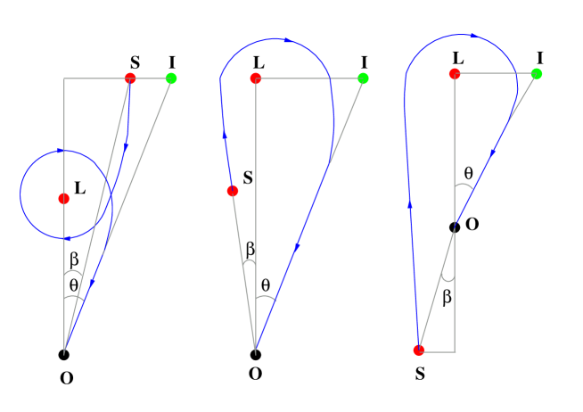
Figure 1: Schematic diagrams of possible lensing geometries.

The observer-source, observer-lens and the lens-source distances, here taken much greater than the horizon radius $r_{h}$, are, in units of $r_{h}$, $d_{os}$, $d_{ol}$ and $d_{ls}$, respectively. Defining $\beta$ as the angular position of the point source and $\theta$ as the angular position of the images (i), both seen from the observer, and $\alpha$ as the deflection angle of the photons, the lens equation [2, 7] has the form:

$$\tan\beta=\tan\theta-c_{3}\left[\tan(\alpha-\theta)+\tan\theta\right],$$ (1)

where $c_{3}=d_{ls}/d_{os}$ for standard lensing and $c_{3}=d_{os}/d_{ol}$ or $c_{3}=d_{os}/d_{ls}$ for cases I and II of retrolensing, respectively. $\beta$ can be taken positive without losing generality. For a spherically symmetric black hole with asymptotically flat metric:

$$ds^{2}=-f(x)dt^{2}+g(x)dx^{2}+h(x)d\Omega^{2},$$ (2)

where $x=r/r_{h}$ is the radial coordinate in units of the horizon radius, the deflection angle $\alpha$ as a function of the closest approach distance $x_{0}$ is given by [8]

$$\alpha(x_{0})=-\pi+\int_{x_{0}}^{\infty}2\left[\frac{g(x)}{h(x)}\right]^{1/2}\left[\frac{h(x)f(x_{0})}{h(x_{0})f(x)}-1\right]^{-1/2}dx.$$ (3)

There are two cases where the deflection angle can be approximated by simple expressions:

• Weak field limit: for $x_{0}\gg x_{ps}>1$ ($x_{ps}$ is the photon sphere radius), a first non null order Taylor expansion in $1/x_{0}$ [9] is made.

• Strong field limit: $\alpha(x_{0})$ diverges when $x_{0}=x_{ps}$, and for $0<x_{0}-x_{ps}\ll 1$, it can be approximated by a logarithmic function [6]:

  $$\alpha(x_{0})\approx-a_{1}\ln(x_{0}-x_{ps})+a_{2},$$ (4)

  where $a_{1}$ and $a_{2}$ are constants.

The weak field limit is used for small deflection angles, as it happens when the lens is a star, a galaxy, or for the weak field images produced by photons with large impact parameters in the case of black holes. The strong field limit is useful to make an approximate analytical treatment of the relativistic images for black hole lenses.

The closest approach distance $x_{0}$ is related with the impact parameter $b$ (in units of the horizon radius) by the equation $b=h(x_{0})/f(x_{0})$ [8], and from the lens geometry $b=d_{ol}\sin\theta$, so $x_{0}$ can be calculated as a function of $\theta$. By putting $x_{0}(\theta)$ in Eq. (4) to have $\alpha(\theta)$, then replacing $\alpha(\theta)$ in Eq. (1), and finally inverting the lens equation (1), the positions of the images are obtained as a function of $\beta$ and the distances involved.

3 Five dimensional Schwarzschild black hole lens

In this Section, a five dimensional Schwarzschild black hole is studied as gravitational lens in the context of braneworlds. The cosmological model adopted is Randall-Sundrum type II [10], which consist of a positive tension brane in a one extra-dimensional bulk with negative cosmological constant. For this black hole, the four dimensional induced metric on the brane is:

$$ds^{2}=-\left(1-\frac{r_{h}^{2}}{r^{2}}\right)dt^{2}+\left(1-\frac{r_{h}^{2}}{r^{2}}\right)^{-1}dr^{2}+r^{2}d\Omega^{2},$$ (5)

where $d\Omega^{2}=d\vartheta^{2}+\sin^{2}\vartheta d\varphi^{2}$ and

$$r_{h}=\sqrt{\frac{8}{3\pi}}\left(\frac{l}{l_{4}}\right)^{1/2}\left(\frac{M}{M_{4}}\right)^{1/2}l_{4},$$ (6)

with $l<0.1$ mm [11] the AdS radius, $l_{4}$ and $M_{4}$, respectively, the Planck length and mass (units in which $c=\hbar=1$ are used). The main features of these braneworld black holes are [12]:

• If $r_{h}\ll l$ they are a good approximation, near the event horizon, of black holes produced by collapse of matter on the brane.

• Primordial black holes in this model have a lower evaporation rate by Hawking radiation than their four dimensional counterparts in standard cosmology, and they could have survived up to present times.

• Only energies of about $1$ TeV are needed to produce black holes by particle collisions instead of energy scales about $10^{16}$ TeV required if no extra dimensions are present. These small size black holes could be created in the next generation particle accelerators or detected in cosmic rays.

Majumdar and Mukherjee [13] considered gravitational lensing in the weak field limit for the black holes discussed above. The positions and magnifications of the relativistic images in the strong field limit are obtained bellow (for more details, see the paper by Eiroa [14]).

3.1 Deflection angle

For the braneworld black hole metric (5) the deflection angle is

$$\alpha(x_{0})=-\pi+2x_{0}^{2}\int_{x_{0}}^{\infty}\left[x^{4}(x_{0}^{2}-1)-x_{0}^{4}(x^{2}-1)\right]^{-1/2}dx,$$ (7)

which, near the photon sphere ($x_{ps}=\sqrt{2}$), can be approximated by [14]

$$\alpha(x_{0})=-\sqrt{2}\ln(x_{0}-\sqrt{2})+\sqrt{2}\ln 4-\pi+O(x_{0}-\sqrt{2}).$$ (8)

Using the impact parameter $b=x_{0}^{2}/\sqrt{x_{0}^{2}-1}$, it takes the form

$$\alpha(b)=-\frac{\sqrt{2}}{2}\ln\left(\frac{b}{b_{ps}}-1\right)+\sqrt{2}\ln(4\sqrt{2})-\pi+O(b-b_{ps}).$$ (9)

3.2 Image positions

In case of high alignment, $\beta\ll 1$, $\theta\ll 1$ and $\alpha$ takes values close to multiples of $\pi$. There are two sets of relativistic images. For the first one, $\alpha=m\pi+\Delta\alpha_{m}$, with $0<\Delta\alpha_{m}\ll 1$, $m=2n$ for standard lensing and $m=2n-1$ for retrolensing ($n\in\mathbb{N}$). The other set of images have $\alpha=-m\pi-\Delta\alpha_{m}$. Then, the lens equation can be approximated by

$$\beta=\theta\mp c_{3}\Delta\alpha_{m},$$ (10)

and from the geometry of the system $b=d_{ol}\sin\theta\approx d_{ol}\theta$, so, defining $\theta_{ps}=2/d_{ol}$, the deflection angle is given by

$$\alpha(\theta)=-c_{1}\ln\left(\frac{\theta}{\theta_{ps}}-1\right)+c_{2}+O(\theta-\theta_{ps}),$$ (11)

where $c_{1}=\sqrt{2}/2$ and $c_{2}=\sqrt{2}\ln(4\sqrt{2})-\pi$. Inverting Eq. (11), making a first order Taylor expansion around $\alpha=\pm m\pi$, and using Eq. (10), the angular position of the $m$-th image is:

$$\theta_{m}=\pm\theta^{0}_{m}+\frac{\zeta_{m}}{c_{3}}(\beta\mp\theta^{0}_{m}),$$ (12)

with

$$\theta^{0}_{m}=\theta_{ps}\left[1+e^{(c_{2}-m\pi)/c_{1}}\right],$$ (13)

and

$$\zeta_{m}=\frac{\theta_{ps}}{c_{1}}e^{(c_{2}-m\pi)/c_{1}}.$$ (14)

For $\beta=0$ (perfect alignment), instead of point images, an infinite sequence of Einstein rings with angular radii

$$\theta^{E}_{m}=\left(1-\frac{\zeta_{m}}{c_{3}}\right)\theta^{0}_{m},$$ (15)

is obtained.

3.3 Image magnifications

As gravitational lensing conserves surface brightness [9], the magnification of the $m$-th image is the quotient of the solid angles subtended by the image and the source:

$$\mu_{m}=\left|\frac{\sin\beta}{\sin\theta_{m}}\frac{d\beta}{d\theta_{m}}\right|^{-1}\approx\left|\frac{\beta}{\theta_{m}}\frac{d\beta}{d\theta_{m}}\right|^{-1};$$ (16)

so, using Eq. (12) and keeping only the first order term in $\zeta_{n}/c_{3}$, it is easy to see that

$$\mu_{m}=\frac{1}{\beta}\frac{\theta^{0}_{m}\zeta_{m}}{c_{3}},$$ (17)

for both sets of images. The total magnification $\mu$ is found by summing up the magnifications of all images; then, for standard lensing $\mu$ is given by

$$\mu=\frac{8}{\beta}\frac{e^{c_{2}/c_{1}}\left(1+e^{c_{2}/c_{1}}+e^{2\pi/c_{1}}\right)}{d_{ol}^{2}c_{1}c_{3}(e^{4\pi/c_{1}}-1)},$$ (18)

and for retrolensing by

$$\mu=\frac{8}{\beta}\frac{e^{(c_{2}+\pi)/c_{1}}\left[1+e^{(c_{2}+\pi)/c_{1}}+e^{2\pi/c_{1}}\right]}{d_{ol}^{2}c_{1}c_{3}(e^{4\pi/c_{1}}-1)}.$$ (19)

When $\beta=0$ the point source approximation fails because the magnifications diverge. Then, an extended source analysis is needed. In this case, it is necessary to integrate over its luminosity profile to obtain the magnification of the images. If the source is an uniform disk $D(\beta_{c},\beta_{s})$, with angular radius $\beta_{s}$ and centered in $\beta_{c}$ (taken positive), the magnification of the $m$-th image is

$$\mu_{m}=\frac{I}{\pi\beta_{s}^{2}}\frac{\theta^{0}_{m}\zeta_{m}}{c_{3}},$$ (20)

where

$$I=2[(\beta_{s}+\beta_{c})E(k)+(\beta_{s}-\beta_{c})K(k)],$$ (21)

with $K(k)=\int_{0}^{\pi/2}\left(1-k^{2}\sin^{2}\phi\right)^{-1/2}d\phi$ and $E(k)=\int_{0}^{\pi/2}\left(1-k^{2}\sin^{2}\phi\right)^{1/2}d\phi$, respectively, the complete elliptic integrals of first and second kind with argument $k=2\sqrt{\beta_{s}\beta_{c}}/(\beta_{s}+\beta_{c})$. Then, the total magnification of an uniform source for standard lensing is

$$\mu=\frac{8I}{\pi\beta_{s}^{2}}\frac{e^{c_{2}/c_{1}}\left(1+e^{c_{2}/c_{1}}+e^{2\pi/c_{1}}\right)}{d_{ol}^{2}c_{1}c_{3}(e^{4\pi/c_{1}}-1)},$$ (22)

and for retrolensing

$$\mu=\frac{8I}{\pi\beta_{s}^{2}}\frac{e^{(c_{2}+\pi)/c_{1}}\left[1+e^{(c_{2}+\pi)/c_{1}}+e^{2\pi/c_{1}}\right]}{d_{ol}^{2}c_{1}c_{3}(e^{4\pi/c_{1}}-1)}.$$ (23)

These expressions always give finite magnifications.

4 Other braneworld black hole lenses

Whisker [15], using the Randall–Sundrum II cosmological model, made a strong field limit analysis for two possible braneworld black hole geometries. The tidal Reissner-Nordström black hole [16] has the metric on the brane:

$$ds^{2}=-\left(1-\frac{2GM}{r}+\frac{Q}{r^{2}}\right)dt^{2}+\left(1-\frac{2GM}{r}+\frac{Q}{r^{2}}\right)^{-1}dr^{2}+r^{2}d\Omega^{2},$$ (24)

where the tidal charge parameter $Q$ comes from the projection on the brane of free gravitational field effects in the bulk, and it can be positive or negative. When $Q$ is positive, it weakens the gravitational field, and if it is negative the bulk effects strengthen the gravitational field, which is physically more natural. This metric has the same properties as the Reissner-Nordström geometry for $Q>0$, there are two horizons, both of which lie within the Schwarzschild horizon. When $Q<0$, there is one horizon, lying outside Schwarzschild horizon. For all $Q$, there is a singularity at $r=0$. The event horizon radius is given by $r_{h}=r_{+}=GM+\sqrt{(GM)^{2}-Q}$ and the radius of the photon sphere by

$$r_{ps}=\frac{3}{2}GM+\frac{1}{2}\sqrt{9(GM)^{2}-8Q}.$$

The strong field limit coefficients $c_{1}$ and $c_{2}$ has to be obtained numerically and they are plotted in Fig. 4 of Ref. [15].

Whisker [15] also proposed as a working metric for the near-horizon geometry the “$U=0$” solution:

$$ds^{2}=-\frac{(r-r_{h})^{2}}{(r+r_{t})^{2}}dt^{2}+\frac{(r+r_{t})^{4}}{r^{4}}dr^{2}+\frac{(r+r_{t})^{4}}{r^{2}}d\Omega^{2},$$ (25)

which has the horizon at $r=r_{h}$. This metric has several differences to the standard Schwarzschild geometry; the horizon is singular (except when $r_{h}=r_{t}$, for which is just the standard Schwarzschild solution in isotropic coordinates), and the area function has a turning point at $r=r_{t}$, that can be either inside or outside the horizon. Another difference, coming from that $g_{tt}\neq g_{rr}^{-1}$, is that the ADM mass and the gravitational mass (defined by $g_{tt}$) are not the same. The photon sphere has radius:

$$r_{ps}=r_{h}+r_{t}+\sqrt{r_{h}^{2}+r_{h}r_{t}+r_{t}^{2}}.$$

The coefficients $c_{1}$ and $c_{2}$ for the metric “U=0” are plotted in Fig. 3 of Ref. [15].

The expressions for the positions and magnifications of the relativistic images obtained in Sec. 3 are valid for these metrics, replacing $c_{1}$ and $c_{2}$ by the values obtained by Whisker, and using the corresponding value of $r_{h}$ to adimensionalize the distances. The metrics considered in this Section, unlike those studied in Sec. 3, can be applied to massive astrophysical black holes. In Ref. [15], the case of the supermassive black hole in the Galactic center was analyzed and the results for the two geometries described above were compared with those corresponding to the standard four dimensional Schwarzschild black hole.

Another related work, using the Arkani-Hamed, Dimopoulos and Dvali braneworld model, is that by Frolov et al. [17]. They found the induced metric on the brane by a Schwarzschild black hole moving in the bulk, and also studied the deflection of light on the brane produced by the black hole.

5 Final remarks

The relativistic images produced by black hole lenses have an angular position about the size of the angle subtended by the photon sphere and they are strongly demagnified, making their observation extremely difficult. In astrophysical scenarios, the observation of these relativistic images is not possible today and it will be a challenge for the next decade. Whisker [15] have shown that a braneworld black hole in the center of our galaxy could have different observational signatures than the four dimensional Schwarzschild one. In the case of small size black holes studied as gravitational lenses by Eiroa [14], the observation of the relativistic images in astrophysical contexts will be even more difficult. But if the braneworld model is correct and these black holes can be produced by next generation of particle accelerators or in cosmic ray showers, it opens up the possibility of observing the phenomena of lensing by black holes in the laboratory.

References

- [1] For a review on braneworld cosmologies see, for example, R. Maartens, Living Rev. Relativity 7, 7 (2004).
- [2] K.S. Virbhadra, and G.F.R. Ellis, Phys. Rev. D 62, 084003 (2000).
- [3] C. Darwin, Proc. Roy. Soc London A 249, 180 (1959).
- [4] V. Bozza, S. Capozziello, G. Iovane, and G. Scarpetta, Gen. Relativ. Gravit. 33, 1535 (2001).
- [5] E.F. Eiroa, G.E. Romero, and D.F. Torres, Phys. Rev. D 66, 024010 (2002)
- [6] V. Bozza, Phys. Rev. D 66, 103001 (2002).
- [7] E.F. Eiroa and D.F. Torres, Phys. Rev. D 69, 063004 (2004).
- [8] S. Weinberg, Gravitation and Cosmology: Principles and Applications of the General Theory of Relativity (Wiley, New York, 1972).
- [9] P. Schneider, J. Ehlers, and E.E. Falco, Gravitational Lenses (Springer-Verlag, Berlin, 1992).
- [10] L. Randall and R. Sundrum, Phys. Rev. Lett. 83, 3370 (1999); Phys. Rev. Lett. 83, 4690 (1999).
- [11] J.C. Long et al, Nature 421, 922 (2003).
- [12] P. Kanti, Int. J. Mod. Phys. A 19, 4899 (2004).
- [13] A.S. Majumdar and N. Mukherjee, astro-ph/0403405.
- [14] E.F. Eiroa, Phys. Rev. D 71, 083010 (2005).
- [15] R. Whisker, Phys. Rev. D 71, 064004 (2005).
- [16] N. Dadhich, R. Maartens, P. Papadopoulos, and V. Rezania, Phys. Lett. B 487, 1 (2000).
- [17] V. Frolov, M. Snajdr, and D. Stojkovic, Phys. Rev. D 68, 044002 (2003).