The Lazarus Project. II. Space-like extraction with the quasi-Kinnersley tetrad

Abstract

The Lazarus project was designed to make the most of limited 3D binary black-hole simulations, through the identification of perturbations at late times, and subsequent evolution of the Weyl scalar $\Psi_{4}$ via the Teukolsky formulation. Here we report on new developments, employing the concept of the “quasi-Kinnersley” (transverse) frame, valid in the full nonlinear regime, to analyze late-time numerical space-times that should differ only slightly from Kerr. This allows us to extract the essential information about the background Kerr solution, and through this, to identify the radiation present. We explicitly test this procedure with full-numerical evolutions of Bowen-York data for single spinning black holes, head-on and orbiting black holes near the ISCO regime. These techniques can be compared with previous Lazarus results, providing a measure of the numerical-tetrad errors intrinsic to the method, and giving as a by-product a more robust wave extraction method for numerical relativity.

I Introduction

The strong-field interaction of black-hole binary systems — from early approach through capture, mutual orbit and eventual merger, to ring-down of the end-state single hole — is expected to be a primary source of gravitational radiation at all frequency scales, and has been a focus of theoretical and numerical attention for forty years. Early perturbative studies Price and Pullin (1994); Pullin (1998); Lousto (2001) and two-dimensional numerical evolutions of axisymmetric binaries (head-on collisions) Hahn and Lindquist (1964); Smarr (1975); Smarr et al. (1976); Čadež (1971, 1974); Anninos and Brandt (1998) were successful in producing late-stage waveforms representing gravitational radiation. However, the move to full 3D simulations of more general initial-data sets has proved extremely difficult. Evolutions using the “standard ADM” 3+1 decomposition of Einstein’s equations and simple zero-shift gauge conditions have stable lifetimes of $\sim 15-30M$ (where $M$ is the total mass of the space-time), far too short a time to complete a useful physical simulations, much less extract the gravitational radiation emitted — the ultimate aim of numerical source simulations.

The Lazarus project Baker et al. (2000, 2002a) was conceived in the context of such limitations. Working under the assumption that the late-evolution 3+1 data can be considered a perturbation of a single Kerr black hole, Lazarus extracts the radiation content everywhere in the numerical domain, and uses it as initial data for a Teukolsky perturbative evolution. In this manner, the original simulation may be extended almost indefinitely, long enough to capture the entire development of the outgoing radiation.

The beginning of the full-numerical simulation can also be interfaced with a far limit approximation method and similar techniques to evaluate a common regime of applicability can be developed Baker et al. (2002a). Here, for the sake of definiteness, we will assume a set of initial data as providing this interface values and focus on the full-numerical / close limit matching.

Lazarus has been very successful, producing the first convergent wave forms Baker et al. (2000, 2001, 2002b, 2004); Campanelli (2005) from 3D evolutions. In most cases, a “plateau” was identified — a range of extraction times $T$ where the emitted energy remained flat and consistent. This plateau begins when the 3+1 data is linearly perturbed from Kerr, and should end only when the radiation has begun to leave the 3+1 numerical domain altogether; at this latter time, Teukolsky extraction will no longer capture the full radiation content. However, the numerical instability of the 3+1 simulation may pollute the Teukolsky initial data for late extraction times. Somewhat surprisingly, such a plateau seems to exist even in situations where a common apparent horizon has yet to form, e.g., short-lived evolutions of so-called “ISCO” (Innermost Stable Circular Orbit) and “pre-ISCO” runs.

Meanwhile, great strides have been made in full 3D simulations over the last decade, due to the casting of Einstein’s equations into more numerically stable formulations Nakamura et al. (1987); Shibata and Nakamura (1995); Friedrich (1996); Frittelli and Reula (1996); Baumgarte and Shapiro (1999); Anderson and York (1999); Alcubierre et al. (2001); Kidder et al. (2001); Sarbach and Tiglio (2002); Shinkai and Yoneda (2002); Lindblom and Scheel (2003); Bona and Palenzuela (2004); Pretorius (2005a), the development of advanced techniques for handling the singularities inherent in black-hole space-times Brandt et al. (2000); Alcubierre et al. (2001, 2004), and the availability of increased computational resources, coupled with mesh-refinement techniques Imbiriba et al. (2004); Fiske et al. (2005); Sperhake et al. (2005); Schnetter et al. (2004); Pretorius and Lehner (2004); Pretorius and Choptuik (2005). The culmination of these advances is several successful evolutions of black-hole-binary systems past the symbolic “one orbit” barrier Brügmann et al. (2004); Pretorius (2005b). For physical systems requiring less than $\sim 100M$ of evolution time to reach a quiescent final state, these improvements enable the direct extraction of radiation from the 3+1 fields, whether through Weyl curvature components or Regge-Wheeler-Zerilli variables Zerilli (1970); Abrahams et al. (1998).

These advances, however, do not lessen the relevance of the Lazarus project. Despite great progress in recent years, it is fair to say that the problem of black-hole binaries is not completely solved. The most astrophysically interesting simulations can still not be evolved long enough to reach their assumed quiescent state. Directly extracted radiation is still calculated at observer locations that lie in the “near-field zone”, or may be under-resolved at more distant locations, and is in general polluted by poor outer-boundary conditions. As long as such limitations exist, there is a place for perturbative methods such as Lazarus. Besides, numerical simulations are still very computationally intensive, and avoiding the last $\approx 100M$ of binary black-hole evolutions means saving days to weeks of supercomputer time.

However, Lazarus makes approximations in its approach. Principal among these is the set of ad hoc choices needed to translate the 3+1 curvature information into a Kerr background + perturbations. The validity of these choices will depend on the data being evolved, and is difficult to quantify a priori.

In this paper, we update the Lazarus project in light of recent work on transverse frames, in a way that may help resolve some of these issues. Beetle et al. Beetle et al. (2005) have proposed a way of identifying the principal directions of a numerical space-time in the 3+1 ADM split. This method — local in nature — allows us to narrow the gap between the numerical tetrad and the Kinnersley tetrad appropriate to the Teukolsky evolution without any background assumptions. When calculated with such a tetrad, the longitudinal Weyl scalars $\Psi_{1}$ and $\Psi_{3}$ will vanish, while the “monopole” scalar $\Psi_{2}$ will take on its Kinnersley-tetrad value, and the transverse scalars $\Psi_{0}$ and $\Psi_{4}$, which carry the radiative degrees of freedom, will differ from their Kinnersley-tetrad values only by a complex factor. This remaining factor can be compensated for, on a known Kerr background in Boyer-Lindquist (BL) coordinates, via a single spin-boost transformation at each point in space.

Although the quasi-Kinnersley frame by no means removes all uncertainties from the problem of radiative extraction, it goes sufficiently far that we expect it to improve the Lazarus procedure considerably. In particular, we expect that the different — and more rigorous — path to Teukolsky waveforms will give us an error estimate for the tetrad dependence of original results, while the robustness of the new technique should allow us to attempt consistent wave extraction from earlier in a numerical evolution.

Additionally, the quasi-Kinnersley frame may achieve much in the simpler problem of direct radiation extraction Beetle et al. (2005); Burko et al. (2005); Beetle and Burko (2002); Nerozzi et al. (2005, 2006). In the past Baker et al. (2002b), we used an approximate tetrad to calculate the Weyl scalar. Since the quasi-Kinnersley tetrad can be constructed locally, without knowing Kerr parameters and BL coordinates, we should now achieve a better approximation to the Kinnersley tetrad during the 3+1 evolution, and thus directly extract waveforms without needing the background data.

The remainder of this paper is laid out as follows: in Section II, we summarize the essentials of the original Lazarus procedure for constructing Cauchy data for Teukolsky evolution, as well as some of the main results from this procedure. In Section III, we review the concepts of transverse frames, and the quasi-Kinnersley frame, and describe the numerical implementation of these concepts in our evolution code. In Section IV, we present comparative results from the application of old and new techniques for three test problems, two of which have already been addressed with original Lazarus Baker et al. (2002b). Discussion of the results obtained, and future work can be found in Section V. Appendix A contains expressions for several quantities related to the evaluation of Weyl scalars in a numerical tetrad in BL coordinates; Appendix B contains perturbative results for the three test cases used in Section IV.

I.1 Notation and Conventions

In the rest of the paper, we shall generally assume a metric signature of $(-,+,+,+)$. Our use of algebraic quantities related to the Kerr-BL solution is non-standard, but consistent with Baker et al. (2002a); we use an additional quantity $\Lambda=r^{2}+a^{2}$ for compactness.

Our sign convention for the definition of the Weyl scalars is such that for the Kerr solution in BL coordinates (and using the Kinnersley tetrad), the only non-vanishing scalar is $\Psi_{2}=M/(r-i\,a\,\cos\theta)^{3}$.

Vector quantities are denoted by an arrow overhead, except for unit vectors, which are instead capped by a circumflex ($\hat{\,}$). Complex conjugation is denoted by an overbar ($\bar{\,}$).

II The Original Lazarus Method

Here we provide a summary of the “original” Lazarus procedure; full details can be found in Baker et al. (2002a), which we shall refer to as Paper I from now on.

We start with a full-numerical 3+1 evolution of a space-time of interest. At some extraction (coordinate) time $T$ — before the simulation crashes due to numerical instabilities — we map the evolved data to a black-hole perturbative evolution code Krivan et al. (1997); Pazos-Ávalos and Lousto (2004). This simpler code can then be evolved stably for as long as is needed to determine the full history of the gravitational radiation generated.

To assess the level of deviation from Kerr at late times in the 3+1 evolution, Baker and Campanelli (2000) introduced an invariant quantity, the speciality index:

$$\mathcal{S}=27\,\mathcal{J}^{2}/\mathcal{I}^{3},$$ (1)

where the two complex curvature invariants $\mathcal{I}$ and $\mathcal{J}$ are essentially the square and cube of the self-dual part, $\mathcal{C}_{abcd}=C_{abcd}+(i/2)\,\epsilon_{abmn}\,C^{mn}_{\;\;\;\;\;\;cd}$, of the Weyl tensor:

$$\mathcal{I}=\mathcal{C}_{abcd}\,\mathcal{C}^{abcd}\;\;{\rm and}\;\;\mathcal{J}=\mathcal{C}_{abcd}\,\mathcal{C}^{cd}_{\;\;\;\;mn}\,\mathcal{C}^{mnab}.$$ (2)

The geometrical significance of $\mathcal{S}$ is that it measures deviations from algebraic speciality (in the Petrov classification of the Weyl tensor). For the unperturbed algebraically special (Petrov type D) Kerr solution, $\mathcal{S}=1$. However, for interesting space-times involving nontrivial dynamics, like distorted black holes, which are in general not algebraically special (Petrov type I), we expect $\mathcal{S}=1+\Delta\mathcal{S}$, and the size of the deviation $\Delta\mathcal{S}\neq 0$, with leading second perturbative order, can be used to assess the applicability of black-hole perturbation theory.

As the expected end-state of most interesting black-hole simulations is a single spinning (Kerr) hole, the perturbative code implements the Teukolsky equation Teukolsky (1973). The Kerr metric in BL coordinates takes the form:

$$ds^{2} = -\left(1-\frac{2\,M\,r}{\Sigma}\right)\,dt^{2}+\frac{\Sigma}{\Delta}\,dr^{2}+\Sigma\,d\theta^{2}$$ (3)

$$+\frac{\Omega}{\Sigma}\,\sin^{2}\theta\,d\phi^{2}-\frac{4\,a\,M\,r}{\Sigma}\,\sin^{2}\theta\,dt\,d\phi,$$

where $\Omega\equiv\Lambda\,\Sigma+2\,M\,a^{2}\,r\,\sin^{2}\theta$, $\Delta\equiv\Lambda-2\,M\,r$, $\Sigma\equiv r^{2}+a^{2}\,\cos^{2}\theta$, and $\Lambda\equiv r^{2}+a^{2}$. In these coordinates, the Teukolsky equation takes the form:

$$\left[{\Lambda^{2}\over\triangle}-a^{2}\sin^{2}\theta\right]{\partial^{2}\psi\over\partial t^{2}}+{4Mar\over\triangle}{\partial^{2}\psi\over\partial t\partial\phi}$$

$$+\left[{a^{2}\over\triangle}-{1\over\sin^{2}\theta}\right]{\partial^{2}\psi\over\partial\phi^{2}}-\triangle^{2}{\partial\over\partial r}\left({1\over\triangle}{\partial\psi\over\partial r}\right)$$ (4)

$$-{1\over\sin\theta}{\partial\over\partial\theta}\left(\sin\theta{\partial\psi\over\partial\theta}\right)+4\left[{a\,(r-M)\over\triangle}+i\,\cot\theta\right]{\partial\psi\over\partial\phi}$$

$$+4\left[{M\,(r^{2}-a^{2})\over\triangle}-\zeta\right]{\partial\psi\over\partial t}+(4\,\cot^{2}\theta+2)\psi=0,$$

where $\psi\equiv\rho^{-4}\,\Psi_{4}$ is the spin-2 Teukolsky function, and $\zeta\equiv r+i\,a\,\cos\theta$. Here $\rho\equiv m^{a}\,l_{a;b}\,\bar{m}^{b}$ is a Newman-Penrose spin coefficient, and $\Psi_{4}$ is a Newman-Penrose Weyl scalar, both calculated using the Kinnersley tetrad.

In the Newman-Penrose formalism Newman and Penrose (1962), there are actually five complex Weyl scalars, formed from contractions of a null tetrad $(l^{a},n^{a},m^{a},\bar{m}^{a})$ with the Weyl tensor:

$$\Psi_{0} \equiv C_{abcd}\,l^{a}\,m^{b}\,l^{c}\,m^{d},$$

$$\Psi_{1} \equiv C_{abcd}\,l^{a}\,m^{b}\,l^{c}\,n^{d},$$

$$\Psi_{2} \equiv C_{abcd}\,l^{a}\,m^{b}\,\bar{m}^{c}\,n^{d},$$ (5)

$$\Psi_{3} \equiv C_{abcd}\,l^{a}\,n^{b}\,\bar{m}^{c}\,n^{d},$$

$$\Psi_{4} \equiv C_{abcd}\,\bar{m}^{a}\,n^{b}\,\bar{m}^{c}\,n^{d}.$$

The $\Psi_{i}$ encode all the vacuum curvature information of the Weyl tensor. As space-time scalars, they are coordinate-independent; however they do depend on the particular null tetrad used. With an appropriate tetrad, in weak-field regions, the interpretation of the $\Psi_{i}$ is as follows: $\Psi_{2}$ embodies the “monopole” non-radiative gravitational field; $\Psi_{1}$ and $\Psi_{3}$ contain the longitudinal radiative degrees of freedom (ingoing and outgoing, respectively), while $\Psi_{0}$ and $\Psi_{4}$ contain the physical transverse radiative degrees of freedom (ingoing and outgoing, respectively) Szekeres (1965). For a numerical space-time that contains a Kerr hole plus perturbative gravitational waves, $\Psi_{4}$ should contain only the appropriate outgoing radiation.

The asymptotic behavior of solutions to the Teukolsky equation is best expressed in terms of the so-called tortoise coordinate $r_{*}$:

$$r_{*} = r+\frac{r_{+}^{2}+a^{2}}{r_{+}-r_{-}}\,\ln\left|\frac{r-r_{+}}{2\,M}\right|-\frac{r_{-}^{2}+a^{2}}{r_{+}-r_{-}}\,\ln\left|\frac{r-r_{-}}{2\,M}\right|,$$

$$r_{\pm} \equiv M\pm\sqrt{M^{2}-a^{2}}.$$ (6)

The point $r_{*}=0$ roughly corresponds to the location of the maximum of the Kerr solution’s scattering potential barrier (see, for example, Eqn (415) and preceding material in Chap. 8 of Chandrasekhar (1983)). For this reason, it should not be crucial to obtain initial data for the Teukolsky equation all the way down to the horizon ($r=r_{+}\Rightarrow r_{*}=-\infty$), as long as we have data for some $r_{*}<0$.

Thus to perform the Teukolsky evolution of radiative data that corresponds to the late-time evolution of our 3+1 initial data, we must identify the parameters $(M,a)$ of the Kerr background, and calculate the radiative Weyl scalar $\Psi_{4}$ using the Kinnersley tetrad. Estimation of the physical parameters can be performed fairly reliably through identification of physical invariants such as the apparent horizon and ADM mass or correcting (iteratively) the initial data parameters by the radiative losses. Evaluating $\Psi_{4}$ using the correct tetrad is less straightforward.

II.1 Tetrad Choice

In BL coordinates, the Kinnersley null tetrad takes the form Kinnersley (1969):

$$\vec{l}_{\rm Kin} = \frac{1}{\Delta}\left[\Lambda,\Delta,0,a\right],$$

$$\vec{n}_{\rm Kin} = \frac{1}{2\Sigma}\left[\Lambda,-\Delta,0,a\right],$$ (7)

$$\vec{m}_{\rm Kin} = \frac{1}{\sqrt{2}\zeta}\left[i\,a\,\sin\theta,0,1,\frac{i}{\sin\theta}\right].$$

Using this tetrad, the spin coefficient $\rho$ takes the form:

$$\rho=(r-i\,a\,\cos\theta)^{-1}=1/\bar{\zeta}.$$ (8)

However, the BL coordinates will not, in general, coincide with the numerical coordinates used in the full 3+1 evolution. We can address this issue in a post-processing step after the evolution, but we must still extract enough curvature information to construct $\Psi^{\rm Kin}_{4}$. Rather than output all the components of the Weyl tensor $C_{abcd}$, it is more efficient to calculate the Weyl scalars with a numerically convenient tetrad, and transform the results to the Kinnersley values during post-processing.

The simpler tetrad we use during evolution is a symmetric null tetrad constructed from the unit hypersurface normal $\hat{\tau}$ and a set of three orthonormal unit spatial vectors $\hat{e}_{(1)}=\hat{e}_{\theta}$, $\hat{e}_{(2)}=\hat{e}_{\phi}$, $\hat{e}_{(3)}=\hat{e}_{r}$, suitably orthonormalized via a Gram-Schmidt procedure:

$$\vec{l}_{\rm num} \equiv \frac{1}{\sqrt{2}}(\hat{\tau}+\hat{e}_{(3)})\;\;,\;\;\vec{n}_{\rm num}\equiv\frac{1}{\sqrt{2}}(\hat{\tau}-\hat{e}_{(3)}),$$

$$\vec{m}_{\rm num} \equiv \frac{1}{\sqrt{2}}(\hat{e}_{(1)}+i\hat{e}_{(2)}).$$ (9)

Similar tetrads have been commonly used in radiation extraction from 3+1 numerical investigations Smarr (1977); Brandt (1996); Fiske et al. (2005); Sperhake et al. (2005), and such a tetrad was used in the earliest investigations of the asymptotic radiative degrees of freedom of the Weyl tensor Szekeres (1965). If we have long-lived 3D numerical evolutions, whose physical domain extends far from the strong-field region, the $\Psi_{4}$ extracted should yield a good measure of the actual outgoing gravitational radiation. We will refer to (II.1) hereafter as the numerical tetrad; explicit formulas for the Kerr-BL Kinnersley tetrad are given in (A).

II.2 Reconstructing Boyer-Lindquist Coordinates

The reconstruction of the BL coordinates $(t,r,\theta,\phi)$ is highly non-trivial. We approach the problem via the following ad hoc steps:

1. assume no polar coordinate distortion;

2. assume that with maximal slicing, numerical time approaches Boyer-Lindquist time;

3. derive the radial coordinate from the equatorial value of numerical $\mathcal{I}$;

4. add a radius-dependent correction to the numerical azimuthal coordinate that zeros out the off-diagonal three-metric component $\gamma_{r\phi}$.

In short:

$$\theta_{\rm BL} = \theta_{\rm num},$$ (10)

$$t_{\rm BL} = t_{\rm num},$$ (11)

$$r_{\rm BL} = \left.\left(3\,M^{2}/\mathcal{I}\right)^{1/6}\right|_{(\theta_{\rm BL}=\pi/2)},$$ (12)

$$\phi_{\rm BL}-\phi_{\rm num} = \phi_{\rm offset}=\int_{\infty}^{r}(\gamma_{r^{\prime}\phi}/\gamma_{\phi\phi})\,dr^{\prime}.$$ (13)

These (last two) coordinate transformations can only be performed as a post-processing step, after the termination of the full 3D numerical evolution.

II.3 Transforming to the Kinnersley Tetrad

For the Kerr-BL metric, we can move from the numerical tetrad to the Kinnersley tetrad by a set of linear transformations governed by the parameters

$$A\equiv a\,\sin\theta\sqrt{\frac{\Delta}{\Omega}}\;,\;F_{A}\equiv\sqrt{\frac{2\,\Sigma}{\Delta}}\;,\;F_{B}\equiv\frac{\sqrt{\Sigma}}{\zeta}.$$ (14)

(Note that $|F_{B}|=1$, since $\zeta\,\bar{\zeta}=r^{2}+a^{2}\,\cos^{2}\theta\equiv\Sigma$.) The specific transformations can be found in Eqn (A); they consist of a combination of type-I and type-II tetrad rotations parametrized by $A$, followed by a type-III “spin-boost” transformation parametrized by the real scaling factor $F_{A}$ and pure-phase complex factor $F_{B}$. This transformation carries over to the Weyl scalars; in particular,

$$\Psi^{\rm Kin}_{4} = \left[(D-1)^{2}\,\Psi^{\rm num}_{0}+4\,i\,A\,(D-1)\,\Psi^{\rm num}_{1}\right.$$ (15)

$$\left.-6\,A^{2}\,\Psi^{\rm num}_{2}-4\,i\,A\,(D+1)\,\Psi^{\rm num}_{3}\right.$$

$$\left.+(D+1)^{2}\,\Psi^{\rm num}_{4}\right]/(4\,F_{A}^{2}\,F_{B}^{2}),$$

where $D\equiv\sqrt{A^{2}+1}$. The equivalent transformations for the other Kinnersley-tetrad scalars can be found in Eqns (A - A).

II.4 Summary of the Original Lazarus Procedure

To summarize, the original Lazarus procedure involves the following steps:

1. construct at every point on the numerical grid a coordinate null tetrad of the form (II.1);

2. calculate the corresponding Weyl scalars $\Psi^{\rm num}_{i}$, the tetrad invariants $\mathcal{I}$, $\mathcal{J}$, and the speciality index $\mathcal{S}$, which we monitor during the entire full-numerical evolution;

3. determine the BL coordinates from the numerical ones via the transformations (10 - 13);

4. use the transformation (15) to obtain the Kinnersley-tetrad $\Psi_{4}$ and $\partial_{t}\Psi_{4}$;

5. evolve the Cauchy data $\psi\equiv\rho^{-4}\,\Psi_{4}$ and $\partial_{t}\psi$ using the Teukolsky equation (II);

6. extract the gravitational radiation information, such as waveforms and total energy radiated at different extraction times $T$.

II.5 Results of Original Lazarus

The original Lazarus procedure as outlined above has been applied extensively to numerical evolutions of black-hole binary data, extending from head-on collisions, grazing collisions and putative circular-orbit data at various orbital separations Baker et al. (2000, 2001, 2002b).

One of the main shortcomings of Lazarus is the ad hoc nature of the coordinate transformations in (10 - 13). Even with data in the linearized regime, Lazarus will be sensitive to how well the numerical space-time satisfies these coordinate assumptions. For instance, we have no guarantee that there is no angular distortion between the numerical and BL radial coordinates (although studies of post-merger apparent horizons have noted a definite tendency of the horizon shape to circularize in numerical coordinates).

An even bolder assumption is that maximal slicing will yield a late-time lapse with the Kerr-BL shape. The Kerr-BL lapse satisfies the maximal slicing equation; however, the numerical lapse also depends on the boundary conditions. In practice, we use Dirichlet boundary conditions, with values equal to that of the Schwarzschild lapse ($M=1$) at the same coordinate position. This choice will give us a lapse shape (and hence numerical time) qualitatively like Kerr-BL; however we only have experimental quantitative experience with the quality of the fit. It can be shown for instance that the numerically obtained lapse quickly takes the form of the BL lapse over points in the exterior of the horizon; the greatest deviations occur within the “potential barrier” at $r_{*}$. A plot demonstrating this for evolved QC0 binary data is shown in Fig. 6 of Paper I.

A complete and unambiguous solution of the coordinate problem is not yet available. Until it is, it seems sensible to work to minimize Lazarus’s coordinate dependence. One obvious area to address is the transformation (15) of the curvature from numerical to Kinnersley tetrad; the numerical Weyl scalars are both mixed and scaled by coordinate-dependent factors. An improvement has been made possible by evaluating the Weyl scalars instead with the quasi-Kinnersley tetrad, which is the subject of the next section.

III Lazarus with the Quasi-Kinnersley Frame

In this section, we review some recent results on transverse frames in numerical space-times, and discuss how they can be used to develop new techniques to improve the Lazarus procedure described in Section II. The main aim is to move closer to the calculation of the actual Kinnersley tetrad during the full 3+1 evolution, and thus to minimize the need for ad hoc coordinate and tetrad correction schemes.

III.1 Transverse Frames and the Quasi-Kinnersley Frame

The Kinnersley tetrad on a Kerr background is transverse – when calculated with this tetrad, the “longitudinal” Weyl scalars $\Psi_{1}$ and $\Psi_{3}$ vanish. This continues to hold for the non-trivial situation of a Kerr hole plus perturbing radiation. However, the coordinate and slicing ambiguity of a generic numerical space-time, even when only perturbatively different from Kerr, mean that this tetrad can be difficult to identify. The Lazarus tetrad-transformation procedure outlined in the previous section will not, in general, yield a transverse tetrad.

A way of identifying transverse tetrads is through finding the eigen-bivectors of the self-dual Weyl tensor $\mathcal{C}_{abcd}$ Beetle et al. (2005) (see also Chapter 4 of D. Kramer and Herlt (1980)). When expressed in a 3+1 decomposition, the Weyl tensor is projected to $C_{ac}\equiv\mathcal{C}_{abcd}\,\tau^{b}\,\tau^{d}$, and the eigen-equation becomes

$$C^{a}_{\;\;c}\,\sigma^{c}\equiv(E^{a}_{\;\;c}-i\,B^{a}_{\;\;c})\,\sigma^{c}=\lambda\,\sigma^{a},$$ (16)

where $E^{a}_{\;\;b}$ and $B^{a}_{\;\;b}$ are the so-called electric and magnetic parts of the Weyl tensor Matte (1953); Smarr (1977). This can be recast by projecting the Weyl tensor onto the orthonormal triad $\{\hat{e}_{(i)}\}$: following D. Kramer and Herlt (1980), we can write (summation is implied over parenthetical indices):

$$C_{ac} = Q_{(i)(j)}\,e_{(i)a}\,e_{(j)c},$$ (17)

$$\sigma^{a} = V_{(i)}\,e_{(i)}^{a},$$ (18)

where $Q_{(i)(j)}$ is a symmetric complex $3\times 3$ matrix whose components are:

$$Q_{(1)(1)} = -\Psi_{2}+(\Psi_{0}+\Psi_{4})/2,$$

$$Q_{(1)(2)} = i(\Psi_{0}-\Psi_{4})/2\;\;,\;\;Q_{(1)(3)}=\Psi_{3}-\Psi_{1},$$

$$Q_{(2)(2)} = -\Psi_{2}-(\Psi_{0}+\Psi_{4})/2,$$ (19)

$$Q_{(2)(3)} = -i(\Psi_{1}+\Psi_{3})\;\;,\;\;Q_{(3)(3)}=2\Psi_{2},$$

and the $\Psi_{i}$ are calculated using the symmetric tetrad (II.1). Then the eigen-equation (16) reduces to

$$Q_{(i)(j)}\,V_{(j)}=\lambda\,V_{(i)}.$$ (20)

The three eigenvalues $\lambda$ of the matrix $Q_{(i)(j)}$ label three transverse frames; the corresponding eigenvectors give the principal directions of the space-time. One of the $\lambda$ is preferred — it will be analytic near the point $\mathcal{S}=1$ in the complex $\mathcal{S}$-plane. The frame related to this $\lambda$ is called the quasi-Kinnersley frame. The preferred $\lambda$ will be numerically equal to $2\times\Psi^{\rm Kin}_{2}$, the value of the monopole Weyl scalar as calculated with the Kinnersley tetrad.

Beetle et al. Beetle et al. (2005) have described the analytic determination of the Weyl eigenvalues. In practice, establishing analyticity of the the eigenvalues is not necessary numerically – Mars Mars (1999) has pointed out that close to Kerr, the eigenvalue with the largest complex norm will give the desired frame; this conclusion has been made more secure by Beetle et al. (2005), who have shown that this is a valid conclusion everywhere in the disc $\|\mathcal{S}-1\|<1$. Instead of following the analytic route, therefore, we use the LAPACK routine zgeev lap to determine numerically the eigenvalues and eigenvectors of $Q_{(i)(j)}$. We select the largest-modulus eigenvalue as the appropriate (quasi-Kinnersley) one.

III.2 Tetrad Reconstruction

Beetle et al. Beetle et al. (2005) lay out a procedure for constructing a tetrad $(l^{a},n^{a},m^{a},\bar{m}^{a})_{\rm qK}$ in the quasi-Kinnersley frame from the eigenvector $V_{(i)}$: first construct $\sigma^{a}$ from (18); normalize it so that $\parallel\vec{\sigma}\parallel=1$; separate into real and imaginary parts: $\sigma^{a}=x^{a}+i\,y^{a}$; construct a third orthogonal vector $z^{a}=\varepsilon^{a}_{\;\;bc}x^{b}y^{c}$; then the new null tetrad vectors are:

$$\vec{l}_{\rm qK} = \frac{|c|}{\sqrt{2}}\left(\parallel\vec{x}\parallel\,\hat{\tau}+\frac{\vec{x}+\vec{z}}{\parallel\vec{x}\parallel}\right),$$ (21)

$$\vec{n}_{\rm qK} = \frac{|c|^{-1}}{\sqrt{2}}\left(\parallel\vec{x}\parallel\,\hat{\tau}+\frac{-\vec{x}+\vec{z}}{\parallel\vec{x}\parallel}\right),$$ (22)

$$\vec{m}_{\rm qK} = \frac{e^{i\,\chi}}{\sqrt{2}}\left(\sqrt{\parallel\vec{x}\parallel^{2}-1}\,\hat{\tau}+\frac{(\vec{z}-i\vec{y})}{\sqrt{\parallel\vec{x}\parallel^{2}-1}}\right),$$ (23)

where $c\equiv|c|\,e^{i\,\chi}$ is an arbitrary spin-boost parameter. We take $|c|=1,\chi=\pi/2$, in order to produce a tetrad that asymptotes to the original numerical tetrad at large distances. The subscript “qK” will refer to this specific choice of $c$ from this point.

If it happens that the eigenvector $\sigma^{a}$ is identically real, $\parallel\vec{x}\parallel=1$, $\parallel\vec{y}\parallel\sim\parallel\vec{z}\parallel\sim\sqrt{\parallel\vec{x}\parallel^{2}-1}=0$ (see Appendix Section B.3 for analytic examples in the “close-slow” limit of binary Bowen-York data). This is not a problem when constructing $\vec{l}_{\rm qK}$ and $\vec{n}_{\rm qK}$; however Eqn (23) will now be undefined. A valid complex null vector $\vec{m}_{\rm qK}$ can still be formed in this case, by replacing the second term in parentheses by any linear combination $\vec{a}+i\,\vec{b}$ of two unit spatial vectors orthogonal to $\vec{x}$. Beetle et al. supply one such choice in Eqn (29) of Beetle et al. (2005). However, the resulting $\vec{m}_{\rm qK}$ at this point will have real and imaginary components that may not match continuously to neighboring points.

In a continuous domain, we could imagine evaluating $\vec{m}_{\rm qK}$ by taking a limit from neighboring points; on a numerical domain (especially in 3D), this is an impractical approach, as (i) it would necessitate knowing in advance which points would need to be interpolated, and (ii) we would need a very dense numerical mesh to carry out such an interpolation. Additionally, there are cases where the pathological points are not isolated, but cover the entire domain. This is the case for Schwarzschild and Brill-Lindquist data. In such cases, no interpolation procedure is possible.

For these reasons, we use an alternative tetrad reconstruction procedure, one that avoids pathologies entirely. We start by following the prescription of Eqns (21 - 22) for the reconstruction of the real null vectors $\vec{l}_{\rm qK}$ and $\vec{n}_{\rm qK}$, as in Beetle et al. (2005); these vary smoothly from point to point, even for pathological regions when $\parallel\vec{z}\parallel=0$.

Next, we take the original numerical complex null vector and split it into real and imaginary parts: $\vec{m}\equiv\vec{X}+i\vec{Y}$. Now starting from these vectors, orthonormalize them according to a set of Gram-Schmidt-like steps. Since $\vec{l}_{\rm qK}$ and $\vec{n}_{\rm qK}$ are already correctly orthonormalized, the remaining requirements are:

$$\vec{m}_{\rm qK}\cdot\vec{l}_{\rm qK} = 0\Rightarrow\vec{X}\cdot\vec{l}_{\rm qK}=0,\;\;\vec{Y}\cdot\vec{l}_{\rm qK}=0,$$

$$\vec{m}_{\rm qK}\cdot\vec{n}_{\rm qK} = 0\Rightarrow\vec{X}\cdot\vec{n}_{\rm qK}=0,\;\;\vec{Y}\cdot\vec{n}_{\rm qK}=0,$$

$$\vec{m}_{\rm qK}\cdot\vec{m}_{\rm qK} = 0\Rightarrow\vec{X}\cdot\vec{Y}=0,\;\;\vec{X}\cdot\vec{X}=\vec{Y}\cdot\vec{Y},$$

$$\vec{m}_{\rm qK}\cdot\vec{\bar{m}}_{\rm qK} = 1\Rightarrow\vec{X}\cdot\vec{X}+\vec{Y}\cdot\vec{Y}=1.$$

The last two equations combine to imply that:

$$\vec{X}\cdot\vec{X}=\vec{Y}\cdot\vec{Y}=1/2.$$

To impose these conditions, we begin with $\vec{X}=\hat{e}_{(1)}/\sqrt{2}$, and enforce the conditions in turn (note that since $\vec{l}_{\rm qK}$ and $\vec{n}_{\rm qK}$ are null, the Gram-Schmidt procedure looks slightly unusual):

$$\vec{X} \rightarrow \vec{X}+(\vec{X}\cdot\vec{l}_{\rm qK})\,\vec{n}_{\rm qK},$$

$$\vec{X} \rightarrow \vec{X}+(\vec{X}\cdot\vec{n}_{\rm qK})\,\vec{l}_{\rm qK},$$

$$\vec{X} \rightarrow \vec{X}/\sqrt{2(\vec{X}\cdot\vec{X})}.$$

In a similar manner, we take $\vec{Y}=\hat{e}_{(2)}/\sqrt{2}$, and enforce orthogonality to $\vec{X}$ just before normalization.

It can be seen that the real and imaginary parts of (23), used as $\vec{X}$ and $\vec{Y}$, pass untouched through the Gram-Schmidt steps above. The choice we make of beginning with the original $\vec{m}$ instead will mean that our final $\vec{m}_{\rm qK}$ differs from (23) by no more than a spin term. Unlike (23), the Gram-Schmidt procedure described can be used everywhere in the numerical domain, and guarantees a smooth behavior moving between neighboring non-pathological and pathological points.

Following the procedure as outlined here exactly reproduces the quasi-Kinnersley tetrad for Kerr-BL, and behaves well for Brill-Lindquist and Bowen-York-type binary data.

III.3 Spin-Boost Fixing and the Kinnersley Tetrad

The tetrad obtained from this procedure will be transverse, and moreover, will be in the same transverse frame as the Kinnersley tetrad — differing only by a Type-III — or spin-boost – transformation. Such a transformation will leave the scalar $\Psi_{2}$ unchanged, but will have a strong effect on the radiative fields $\Psi_{0}$ and $\Psi_{4}$, scaling and mixing polarizations.

Lacking an unambiguous and natural way to lock down the spin-boost needed to obtain the Kinnersley tetrad from the quasi-Kinnersley frame member, we return to our knowledge of the Kerr background. It can be shown that for Kerr-BL, the null tetrad produced from the correct transverse eigenvector (by following the construction in Beetle et al. (2005)) is

$$\vec{l}_{\rm qK} = \frac{1}{\sqrt{2\Delta\Sigma}}\left[\Lambda,\Delta,0,a\right],$$

$$\vec{n}_{\rm qK} = \frac{1}{\sqrt{2\Delta\Sigma}}\left[\Lambda,-\Delta,0,a\right],$$ (24)

$$\vec{m}_{\rm qK} = \frac{-i}{\sqrt{2\Sigma}}\left[ia\sin\theta,0,1,\frac{i}{\sin\theta}\right],$$

that is, the new tetrad is related to the Kinnersley tetrad (II.1) via:

$$\vec{l}_{\rm Kin} = \sqrt{\frac{2\Sigma}{\Delta}}\vec{l}_{\rm qK}\;\;,\;\;\vec{n}_{\rm Kin}=\sqrt{\frac{\Delta}{2\Sigma}}\vec{n}_{\rm qK},$$

$$\vec{m}_{\rm Kin} = \frac{\bar{\zeta}}{\sqrt{\Sigma}}\vec{m}_{\rm qK}.$$ (25)

This implies that the corresponding Kinnersley-tetrad $\Psi_{4}$ can be obtained simply from:

$$\Psi^{\rm Kin}_{4}=\Psi^{\rm qK}_{4}/F_{A}^{2}\,F_{B}^{2}.$$ (26)

Note that this transformation, unlike (15) for original Lazarus, does not involve any mixing of the Weyl scalars.

III.4 Summary of the New Procedure

Thus the new Lazarus procedure involves the following sequence of steps:

1. construct at every point on the numerical grid a coordinate null tetrad of the form (II.1);

2. calculate the corresponding Weyl scalars $\Psi^{\rm num}_{i}$, the tetrad invariants $\mathcal{I}$, $\mathcal{J}$, and the speciality index $\mathcal{S}$, which we monitor during the full-numerical evolution;

3. construct the matrix $Q_{(i)(j)}$ (III.1), and find its eigenvalues and eigenvectors;

4. pick the eigenvalue $\lambda$ with the largest (complex) magnitude;

5. use the corresponding unit-norm eigenvector $\vec{V}$ to form the principal (complex) spatial vector $\sigma^{a}\equiv V_{(i)}\,e^{a}_{(i)}$;

6. construct a new null tetrad according (21), (22), and the pathology-avoiding steps following;

7. recalculate the Weyl scalars with this new tetrad;

8. determine the BL coordinates from the numerical ones via the transformations (10 - 13);

9. use the transformation (26) to produce the Kinnersley-tetrad $\Psi_{4}$ and $\partial_{t}\Psi_{4}$;

10. evolve the Cauchy data $\psi\equiv\rho^{-4}\,\Psi_{4}$ and $\partial_{t}\psi$ using the Teukolsky equation (II);

11. extract the gravitational radiation information, such as waveforms and total energy radiated at different extraction times $T$.

In the above, only steps (i)-(vii) can be carried out in the full-numerical evolution; step (ix) is a post-processing step, as it still involves knowledge of the appropriate Kerr background parameters ($M$,$a$), and BL coordinates. While the new Lazarus approach outlined above does not solve this problem, it reduces the dependence of the Teukolsky data on the tetrad choices, by reducing the number of functions that depend on the BL coordinates.

IV Numerical Evolutions

We have applied the new transverse-frame-based techniques outlined above to three numerical regimes of increasing complexity: Bowen-York data for one spinning hole, Brill-Lindquist data for the head-on collision of two black holes, initially at rest, and transversely boosted binary Bowen-York data, representing an “Innermost Stable Circular Orbit”. Two of these data sets were already investigated in detail using the existing Lazarus approach in Baker et al. (2002b); our new techniques should allow some additional estimate on their validity.

The results have been obtained from 3D evolutions performed with the standard ADM decomposition of Einstein’s equations York (1979), together with zero shift and maximal slicing lapse. It may be objected that this combination of evolution systems and gauge conditions is not state-of-the-art. More sophisticated and stable systems are in wide use at present, and we would certainly expect them to produce much longer-lived stable full 3D evolutions. In particular, a new numerical-relativity framework (LazEv) has been successfully developed Zlochower et al. (2005) and is currently available to the authors of this paper; it allows for evolutions of black-hole binaries using higher-order finite differencing, with the BSSN formulation of Einstein’s equations and dynamical gauge conditions. Nevertheless, we have two reasons for using the “ADM + maximal slicing + zero shift” combination: First, this combination was that used for the original Lazarus tests; if we desire a fair comparison of old and new methods, focused on the new tetrad methods we have developed, use of more modern and stable evolution methods will only obscure the results. Second, the introduction of more sophisticated gauges will necessitate the reconsideration of the the numerical-to-Kerr-BL coordinate transformation. In particular, the use of other lapse evolution schemes may lead to a lapse shape significantly different to the maximal and Kerr-BL shapes. Also, the presence of a non-zero shift vector will alter the azimuthal-angle relationship (13).

We carried out the coding and testing of the concepts presented here using the Cactus Cac framework. Post-processing of the 3D data and subsequent Teukolsky evolution was done with stand-alone codes.

In these evolutions, we were also monitoring the appearance of a single merged black hole using the apparent horizon finder AHFinderDirect Thornburg (2004).

IV.1 Spinning Bowen-York Data

The Bowen-York solution Bowen and York (1980) representing a single black hole with angular momentum $J$ should resemble — once the Hamiltonian constraint has been solved — a single Kerr black hole with gravitational radiation on top. The rotational symmetry of the solution about its spin axis (the coordinate polar or $z$ axis) means that only radiation with $m=0$ will be present, and that there should be no net loss of angular momentum through gravitational radiation. Some analytic treatment of this data is presented in the Appendix Section B.1, based on Gleiser et al.’s perturbative analysis Gleiser et al. (1998).

In an early numerical investigation of the suitability of such data for Lazarus, we evaluated this data — using a full-numerical solution to the constraints — and extracted the radiation content of the initial data via the new Lazarus method. We found that for small spins ($J/M^{2}\lesssim 0.2$), a spatial resolution of up to $M/80$ would be necessary to identify unambiguously the leading-order real ($\ell=2$) and imaginary ($\ell=3$) parts of the Teukolsky function. Such a resolution is not feasible for a unigrid run, if the outer boundaries are to be outside the strong-field region. For this reason, we have used a larger initial spin for full-numerical simulations.

This data was implemented on the initial numerical slice in Cactus, with bare mass $m=0.858\,M_{\rm ADM}$, and spin angular momentum $J=0.553\,M_{\rm ADM}^{2}$; after numerical solution of the Hamiltonian constraint, the ADM mass of the initial data was $M_{\rm ADM}=1.0$. To extend the physical domain, we used a “transition fisheye” radial transformation of the numerical coordinates Baker et al. (2002a). The explicit form we used in this paper can be found in Eqn (114) of Alcubierre et al. (2003), with parameters $(a=7,s=2,r_{0}=7)$; this produced a physical radial extent of $33.6\,M$ from a numerical radial extent of $10.79M$. We used three spatial resolutions — $M/12$, $M/18$ and $M/24$. Because the solution below the $x$-$y$ plane is trivially related to that above the plane, we were able to evolve the upper bitant only. The 3+1 simulation died due to numerical instabilities before $25\,M$ of coordinate time at the coarsest resolution, before $19\,M$ at the medium resolution, and before $18\,M$ at the finest resolution.

For such a weak-field case, we expect the Lazarus techniques to be applicable from a very early time. An apparent horizon is already present in the initial data, and Fig. 1 shows the value of the (real part of the) speciality index $\mathcal{S}$ along the $x$ axis outside the horizon, evaluated at several times in the evolution. At all times after the initial slice, the deviation from the Kerr value of $\mathcal{S}=1$ is at most $\sim 2\%$. Thus the spinning BY data should certainly be within the linearized regime almost immediately. (Nevertheless, Lazarus results will be sensitive to how well the numerical space-time satisfies the coordinate assumptions of Section II.2.)

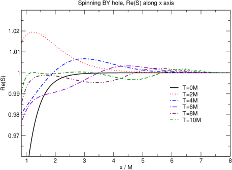
Figure 1: The real part of the $\mathcal{S}$ invariant along the $x$ axis for Spinning BY data, at different extraction times $T$.

We analyzed the evolved data with both the original and new Lazarus approaches. At every $M$ of coordinate time evolution, the Weyl scalars were calculated using both the original and new tetrads, then mode-decomposed and saved to file. We post-processed this data to produce the Teukolsky Cauchy data $(\psi,\partial_{t}\psi)$, which was then evolved using a code that solves the Teukolsky Equation. The total extracted energy as a function of extraction time $T$ is shown in Fig. 2. Between extraction times of $1M$ and $5M$, we see an emitted-energy plateau at around $1.25\times 10^{-4}\,M$, common to both original and new Lazarus, with a deviation of $\sim 3.5\%$ between old and new values.

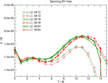
Figure 2: Total radiated energy for Spinning BY data as calculated from original (L1) and new (L2) Lazarus methods, as a function of extraction time $T$.

We would expect that once we have entered an energy plateau, we should remain there, at least until the radiation has left the outer boundary of the full-numerical domain. However, for later extraction times, from $6M$ to $10M$, we see a monotonic decrease in emitted energy, leading to a low point of $\sim 0.88\times 10^{-4}\,M$, a drop of $\sim 30\,\%$. This degradation is common to both original and new Lazarus.

This behavior may be an artifact of the underlying ADM evolution system, or other aspects of the Lazarus procedure; even for the relatively high spin chosen here, spinning Bowen-York is a weak source of gravitational radiation, and presumably extremely sensitive to details in the simulation. Further investigation with newer, more stable and accurate, evolution systems may illuminate the situation.

The level of emitted energy is consistent with the full-numerical results shown in  Dain et al. (2002) and the perturbative results of Gleiser et al. Gleiser et al. (1998): they obtain a total emitted energy of $\sim 2.5\times 10^{-4}\,M$ for a spin of $J_{\rm ADM}=0.55\,M^{2}$. Although significantly larger than our peak energy of $\sim 1.25\times 10^{-4}\,M$, it falls into the “factor of two” accuracy the authors assess for their method at high spins.

Selected Teukolsky-evolved waveforms (the rescaled Weyl scalar $\Psi_{4}$), measured at $(r_{*}=30\,M,\theta=0)$, are shown in Fig. 3. The waveforms shown are for the new tetrad method only (old-method waveforms are indistinguishable). There is good agreement especially between extraction times $T=3\,M$ and $5\,M$. For later extraction times, the waveforms lose coherence after a few wavelengths.

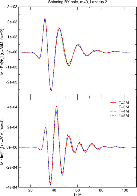
Figure 3: Evolution of the $m=0$ Spinning BY waveform for the new (L2) Lazarus method, evaluated at $r_{*}=30\,M$ along maximal amplitude directions: $\theta=90^{\circ}$ for $Re(\Psi_{4})$, $\theta=45^{\circ}$ for $Im(\Psi_{4})$. The five curves represent five different extraction times in the energy plateau of Fig. 2.

IV.2 Brill-Lindquist Data

This test revisits the case of head-on collisions of Brill-Lindquist data, treated previously in the Lazarus context Baker et al. (2000, 2002b). Data of this type was studied in a perturbative form in Ref. Abrahams and Price (1996); based on the full-numerical results available at the time, perturbative results overestimate the total emitted energy for large separations. Qualitatively similar conclusions can be drawn using Misner initial data Lousto (2001).

The specific initial data chosen has two holes with equal bare masses $m=0.50\,M$, with a coordinate separation along the $y$ axis of $2.303\,M$, yielding a proper horizon-to-horizon separation of $L=4.9M$, and no linear or angular momentum (this data set was referred to as “$P=0$” in Baker et al. (2002b)). The symmetry of the problem allows us to use only the first octant of the numerical grid during evolution. Otherwise, the grid extent and fisheye transformation were identical to those for the spinning Bowen-York case above.

Again, we evolved the initial data using the “standard ADM” evolution scheme with maximal slicing and zero shift. The finest resolution run crashed due to numerical instabilities before $20M$ of coordinate time. Nevertheless, a common apparent horizon was found at coordinate time $t\approx 8\,M$, and there is reason to believe that a common event horizon is present from $t\approx 3\,M$ Diener and a continuous potential barrier surrounding the strong-field region around even earlier. We show the evolution of the speciality index $\mathcal{S}$ in Fig. 4. While deviations from unity are always large near the punctures, the overall deviation outside the eventual common horizon location have dropped to below $10\%$ by $T\approx 8\,M$, indicating we have entered the linear regime.

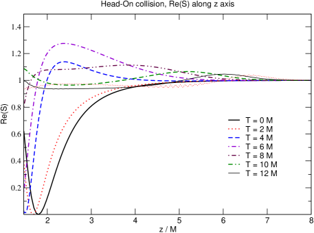
Figure 4: The $\mathcal{S}$ invariant along the $z$ axis for Head-On data, at different extraction times $T$.

Fig. 5 shows the total radiated energy from the Teukolsky evolution, as a function of the extraction time $T$ for original and new methods, for the $m=0$ (upper panel) and $m=+2$ (lower panel) modes. For both sets of modes, original and new Lazarus deviate at early extraction times. While the original Lazarus results reproduce what was seen in Fig. 5 of Baker et al. (2002b) — the radiated energy reaches a crude plateau between extraction times of $4M$ and $10M$ — the new-tetrad-produced energy reaches a level plateau only after $7\,M$. After this time, both methods agree well until $10\,M$, but with a noticeably more level plateau in the weaker $m=0$ curve for the new tetrad.

Table 1 compares the total energy calculated with old and new Lazarus with a direct-extraction energy taken from Zlochower et al. (2005) (this extraction was from a rather close detector position, $r_{*,obs}\approx 7.46\,M$). While both Lazarus figures differ from the direct result, the new Lazarus plateau – measured from $T=8\,M$ and $T=11\,M$ – has less than half the standard deviation of old Lazarus, indicating a more stable plateau.

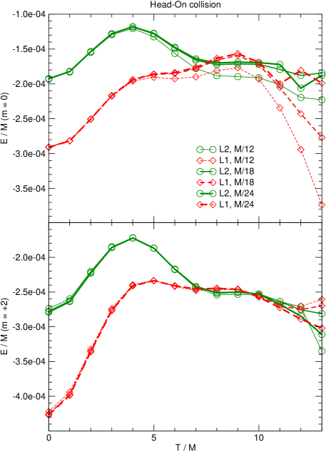
Figure 5: Radiated energy for Head-On collision as calculated from original (L1) and new (L2) Lazarus methods, as a function of extraction time $T$. Note the extension of the plateau with increasing resolution.

Table 1: Comparison of emitted $E$ for Head-On collision. Direct results ($r_{*,obs}=7.46\,M$) are from Zlochower et al. (2005). $\bar{E}$ and $\sigma_{E}$ are the mean and standard deviation from four plateau values.

Source	$|\bar{E}|/M$	$\sigma_{E}/M$
	$\times 10^{-4}$	$\times 10^{-4}$
Direct	6.6	—
L1 ($8-11M$)	6.827	0.446
L2 ($8-11M$)	6.811	0.179

Fig. 6 shows the dominant-mode ($m=+2$) Lazarus waveform for the Head-On collision, measured at $(r_{*}=30\,M,\theta=0)$. While the difference between curves for early extraction times can give an idea of the uncertainties of the method when nonlinearities are present the agreement at later times shows when a safe, linear regime is reached.

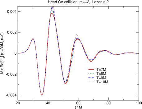
Figure 6: Evolution of the $m=+2$ Head-On waveform for the new (L2) Lazarus method, evaluated at $(r_{*}=30\,M,\theta=0)$.

IV.3 QC0 Data

The final test of our method again revisits initial data treated in Baker et al. (2002b): Bowen-York binary black-hole data, where the holes have zero spin, but are boosted in a direction transverse to their separation, to achieve a net orbital angular momentum $J$.

Khanna et al. Khanna et al. (1999) investigated such data to first perturbative order, through Zerilli and Teukolsky schemes. The emitted energy curves from the two methods diverge at the level $J/M^{2}\approx 0.4-0.5$, and this the authors take as the limit of applicability of linear perturbative theory. At the highest analyzed spin, $J/M^{2}=0.6$, the Teukolsky- and Zerilli-calculated energies are $\sim 8\times 10^{-3}\,M$ and $\sim 5\times 10^{-3}\,M$ respectively.

Here, we use the binary Bowen-York data with equal bare masses $m=0.45\,M$, located at coordinate positions $y=\pm 1.1515\,M$, and with Bowen-York “boosts” $P=\pm 0.335\,M$ in the $x$ direction. These result in a physical throat-to-throat separation $L=4.9\,M$, and a total ADM angular momentum $J=0.77\,M^{2}$. We refer to this data set as “QC0”, following the classification scheme of Baker et al. (2002b); it was originally suggested by Baumgarte Baumgarte (2000) (adapting Cook’s “effective potential” method Cook (1994) to punctures) as a model for the so-called Innermost Stable Circular Orbit (ISCO) of two equal-mass black holes.

In contrast to the two previous test cases, numerical instabilities will kill the QC0 data evolution before a single common apparent horizon has appeared (though a common event horizon may already be present). Thus Lazarus extraction and evolution of Teukolsky data would not appear to be completely justified at any time. Nevertheless, Baker et al. (2002b) found a small plateau in the emitted energy, indicating a range of extraction times where the system has effectively linearized prior to the simulation’s crash.

For this data, the Lazarus procedure was carried out initially using a zeroth-order parameter estimate taken from the ADM energy and angular momentum of the initial data: $M=1$, $a=0.77$. However, since the emitted energy and angular momentum were at the level of a few percent of the total, the subsequent drop in background mass and spin might be significant. For this reason, we iterated the method with suitably reduced background mass and spin parameters: $M=0.974$, and $a=0.675/M=0.693$.

To demonstrate how quickly the system appears to relax to Kerr, we show in Fig. 7 the $\mathcal{S}$ invariant along the $x$ and $z$ axes. Along the $z$ axis, $\mathcal{S}$ clearly takes time to settle down, only uniformly falling within $[0.5,2.0]$ rather late in the simulation, after $T=8\,M$.

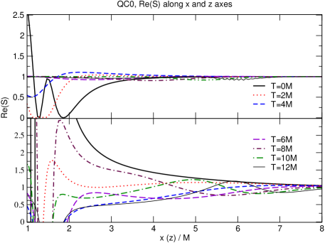
Figure 7: The $\mathcal{S}$ invariant along the $x$ (upper) and $z$ (lower) axes for QC0 data, at different extraction times $T$.

Fig. 8 shows the emitted energy and angular momentum, respectively, for both original and new Lazarus methods (the dominant $m=+2$ mode waveform is plotted for old and new Lazarus in Fig. 9 and Fig. 10, respectively). The original Lazarus results can be found in Fig. 22 of Baker et al. (2002b) (note that the latter figure contains the total energy summed across $m$ modes). There is significant deviation between original and new Lazarus results up to the extraction time of $T\approx 6\,M$. The two methods agree well for $T\in[7\,M,8\,M]$, but begin to diverge again around the time new Lazarus develops plateau values of around $1.1\times 10^{-2}\,M$ and $4.25\times 10^{-2}\,M^{2}$ for the emitted energy and angular momentum, in the mode $m=+2$, respectively. Working with the more time-resolved data of the inserts in Fig. 8, we have identified the plateaus for old and new Lazarus, and calculated the means and standard deviations. We present these in Table 2, along with direct-extraction results ($r_{*,obs}=14.03\,M$) from Campanelli et al. (2005). While both old and new means differ from the direct-extraction figures, new Lazarus’s plateau is flatter.

Because the QC0 data takes time to plunge to a single hole, the onset of linearization will be delayed relative to, for instance, the head-on case. The fact that the observed plateau does not persist for longer than $\sim 2\,M$ is a consequence of the instability of the the simple combination of “ADM + maximal lapse + zero shift” we have used in our full-numerical evolutions here. In this sense, QC0 + ADM is a “marginal” Lazarus case; to establish the plateau unambiguously will require evolutions that last for several more $M$. This will necessitate more advanced evolution systems and gauges, and is addressed in the Discussion below.

Table 2: Comparison of emitted $E$ and $J$ for QC0 merger. Direct results ($r_{*,obs}=14.03\,M$) are from Campanelli et al. (2005). $\bar{E}$, $\bar{J}$ are the means and $\sigma_{E}$, $\sigma_{J}$ the standard deviations from five plateau points (indicated in first column).

Source	$|\bar{E}|/M$	$\sigma_{E}/M$	$|J|/M^{2}$	$\sigma_{J}/M^{2}$
	$\times 10^{-2}$	$\times 10^{-2}$	$\times 10^{-2}$	$\times 10^{-2}$
Direct	$2.8\pm 0.2$	—	$11.0\pm 1.0$	—
L1 ($9.0-11.0M$)	2.570	0.067	9.493	0.434
L2 ($8.5-10.5M$)	2.422	0.031	8.553	0.175

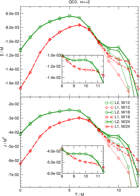
Figure 8: $m=+2$ radiated energy and angular momentum for QC0 data as calculated from original (L1) and new (L2) Lazarus methods, as a function of extraction time $T$.

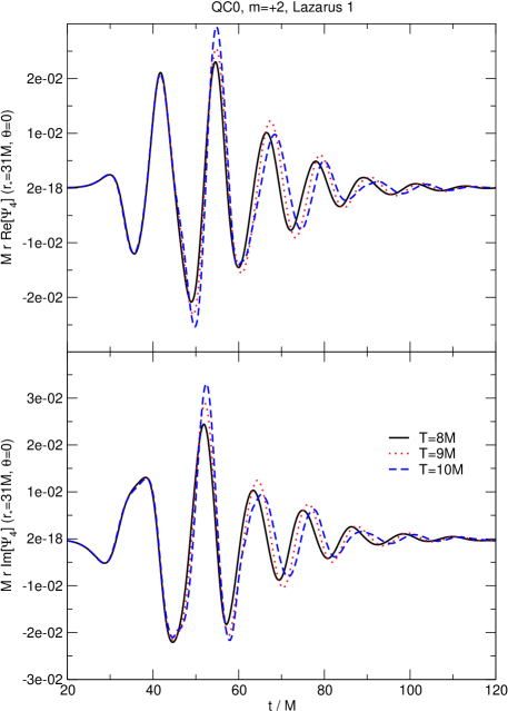
Figure 9: The two polarizations of the $m=+2$ QC0 waveform for the original (L1) Lazarus method, evaluated at $(r_{*}=31\,M,\theta=0)$.

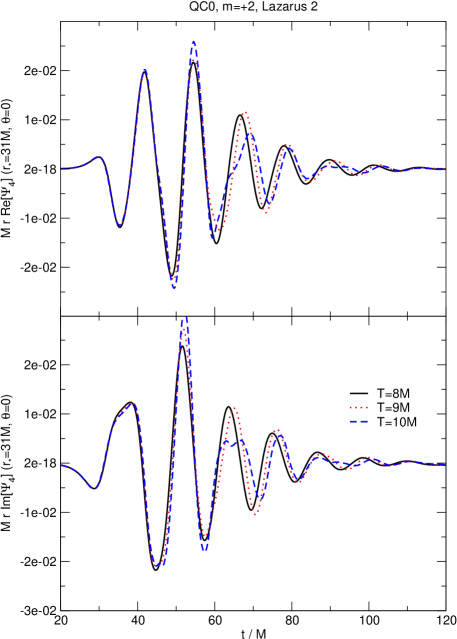
Figure 10: The two polarizations of the $m=+2$ QC0 waveform for the new (L2) Lazarus method, evaluated at $(r_{*}=31\,M,\theta=0)$.

V Discussion

The original Lazarus method was a successful synthesis of full-numerical and perturbative methods in numerical relativity. It was responsible for the production of the first waveform for black-hole binary mergers and close orbits, before these regimes were accessible to a complete full-numerical treatment.

We have presented in this paper the first in a series of proposed improvements to the Lazarus method — improvements which will, we hope, make Lazarus more ambitious in its reach, and more rigorous in its grasp. The developments herein have focused on the important area of tetrad determination. We can now obtain — in the “real time” of the full-numerical evolution — a transverse tetrad that will differ from the Kinnersley tetrad only by a spin-boost.

We described in Section III how this new method of tetrad determination can be incorporated into the Lazarus project, eliminating the artificial mixing of monopolar, longitudinal and transverse modes that was necessary in original Lazarus. To test this new aspect, we have applied it on the same footing as original Lazarus — to the short-lived ADM evolutions of three different types of black-hole data.

Our numerical results with this method, reported in IV, have allowed us to test this mode mixing for the first time. The good agreement between old and new methods for the single Spinning Bowen-York and Head-On cases, where linearization is seen well before code break-down, can be seen as a validation of the applicability of the original Lazarus mixing formulas; additional evolution time may be needed to resolve the marginal case of QC0 data satisfactorily. In contrast, the areas of difference — seen for instance, before $T=7\,M$ in Fig. 5 for the Head-On case — indicate better where our assumption of linear deviation from Kerr may not have been justified. With this alternative path to the Kinnersley tetrad in Lazarus, we have produced error estimates for the tetrad construction procedure; we can estimate the contribution that errors in this procedure make to the overall uncertainty in Lazarus energies. It should be noted, however, that this error is unlikely to dominate the total uncertainty in emitted energies. Comparison of Lazarus (both old and new) results with more direct extraction techniques, shown in Tables 1 and 2, indicate that other important factors must still be addressed. A reasonable estimate of theoretical error in waveforms will be needed for their application to analysis of gravitational-wave detector signals in the future.

For the next stage in the Lazarus project, we plan to use modern evolution schemes, such the one provided by the LazEv framework Zlochower et al. (2005), which are more stable and accurate than ADM. LazEv currently supports higher-order finite differencing for the BSSN formulation of Einstein’s equations with the choice of several dynamical gauge conditions, and should allow for extended energy plateaus, extending from the time of first linearization of the system until the time the radiation leaves the system. This added full-numerical evolution time will aid in the unambiguous identification of the linearization time for marginal cases such as “QC0” above.

At present, it is unclear how to relate Boyer-Lindquist time to the numerical time developed with standard numerical gauges. Maximal slicing was discussed in Section II.5; future refinements of this may use analytic insights into the late-time shape of the maximal lapse (see Reimann and Brügmann (2004) for work on maximal slicings of Schwarzschild). Commonly used dynamic slicings (e.g., “1+log” slicing) ensure a lapse function with the same qualitative shape, falling smoothly off to unity at large distances. The exact shape will vary greatly in the near-field region, however, and this will affect both old and new Lazarus; this is an interesting problem, which we hope to address in future work.

Treatment of the shift is decoupled from the lapse in the Lazarus approach; the shift correction via adjustment of $\phi$ is independent of the slicing analysis. Co-rotating coordinates can already be accommodated with this method. We expect to treat more complicated evolution shifts in a similar way.

The quasi-Kinnersley frame has further useful applications. For direct radiation extraction at a finite observer location in the 3D numerical grid. It also provides a closer interpretation in terms of radiation for 3-dimensional visualizations. Originally one uses the numerical tetrad to evaluate $\Psi_{4}$. In order to give this a direct interpretation in terms of radiation, one implicitly assumes that the observer is sufficiently far from the strong-field region that the background space is almost flat, and the numerical tetrad is a good approximation to Kinnersley.

With the quasi-Kinnersley frame, we can get much closer to the true Kinnersley form at finite observer locations. This should supply us with a more robust waveform at distant locations, and allow us to approach the near-field zone with greater confidence. While impracticable for short-lived ADM evolutions, modern evolution systems should produce several periods of directly extracted waveforms at different extraction radii. Outer-radius waveforms may be compared with Lazarus results; inner waveforms may be compared with outer ones as a test of the quality of strong-field waveforms in general.

Aside from the longer full-numerical evolution times, we plan to investigate further several issues to improve the generality of Lazarus.

The transformations used to extract Boyer-Lindquist coordinates from the numerical ones perform well, but there is much room for improvement. One obvious — and theoretically well-founded — step that can be taken is relaxing the assumption that there is a one-to-one relationship between the numerical radial coordinate $R_{\rm num}$ and the Boyer-Lindquist $r$. Since we know the theoretical form of the invariant $\mathcal{I}$ as a function of $(r,\theta)$, we can imagine using $\mathcal{I}$ everywhere to derive both $r$ and $\theta$. We have performed initial investigations of this possibility, but found that the off-equator radial transformation derived does not reach sufficiently close to the horizon, at least for the most difficult cases, such as the QC0. Longer full-numerical evolutions may improve the performance of this technique, as a horizon appears and circularizes. We also plan to revisit the choice of the time slicing as this might be crucial to process longer-term fully nonlinear evolutions.

Appendix A Numerical-Kinnersley Transformations for Kerr Data

In Boyer-Lindquist (BL) coordinates, the numerical tetrad — defined by (II.1) with orthonormalized spherical coordinate directions for the $\hat{e}_{(i)}$ — takes the form:

$$\vec{l}_{\rm num} = \frac{1}{2}\left[\sqrt{\frac{\Omega}{\Delta\Sigma}},\sqrt{\frac{\Delta}{\Sigma}},0,\frac{2aMr}{\sqrt{\Delta\Omega\Sigma}}\right],$$

$$\vec{n}_{\rm num} = \frac{1}{2}\left[\sqrt{\frac{\Omega}{\Delta\Sigma}},-\sqrt{\frac{\Delta}{\Sigma}},0,\frac{2aMr}{\sqrt{\Delta\Omega\Sigma}}\right],$$ (27)

$$\vec{m}_{\rm num} = \frac{1}{2}\left[0,0,\frac{1}{\sqrt{\Sigma}},\frac{i}{\sin\theta}\,\sqrt{\frac{\Sigma}{\Omega}}\right].$$

Such a tetrad will differ strongly from the Kinnersley tetrad; as a consequence, all Weyl scalars calculated from it will be non-zero. For Kerr-BL, these values will be:

$$\Psi_{0}=\Psi_{4} = -\frac{M}{2\Omega\bar{\zeta}^{3}}[3(\Lambda^{2}-\Omega)].$$

$$\Psi_{1}=-\Psi_{3} = -\frac{M}{2\Omega\bar{\zeta}^{3}}[3i\Lambda\sqrt{\Lambda^{2}-\Omega}].$$ (28)

$$\Psi_{2} = -\frac{M}{2\Omega\bar{\zeta}^{3}}[-(3\Lambda^{2}-\Omega)].$$

For Kerr-BL coordinates, the numerical null tetrad (A) used in 3+1 numerical calculations can be transformed to the Kinnersley tetrad (II.1) via a combination of null rotations and spin-boosts:

$$\vec{l}_{\rm Kin} = \frac{F_{A}}{2}\left\{(D+1)\,\vec{l}_{\rm num}+(D-1)\,\vec{n}_{\rm num}\right.$$

$$\left.-i\,A\,(\vec{m}_{\rm num}-\vec{\bar{m}}_{\rm num})\right\},$$

$$\vec{n}_{\rm Kin} = \frac{F^{-1}_{A}}{2}\left\{(D-1)\,\vec{l}_{\rm num}+(D+1)\,\vec{n}_{\rm num}\right.$$ (29)

$$\left.-i\,A\,(\vec{m}_{\rm num}-\vec{\bar{m}}_{\rm num})\right\},$$

$$\vec{m}_{\rm Kin} = \frac{F_{B}}{2}\left\{(D+1)\,\vec{m}_{\rm num}-(D-1)\,\vec{\bar{m}}_{\rm num}\right.$$

$$\left.+i\,A\,(\vec{l}_{\rm num}+\vec{n}_{\rm num})\right\}.$$

Note that this is a corrected form of the transformations that appeared in Eqns (5.9a-c) of Paper I.

The dependence of the Kinnersley-tetrad $\Psi_{4}$ on the the numerical-tetrad scalars was given in (15), for perturbations of Kerr-BL coordinates. The following are the corresponding expressions for the remaining Kinnersley Weyl scalars (the mixing function $A$ and spin-boost functions $F_{A}$ and $F_{B}$ are given by (14), and $D\equiv\sqrt{A^{2}+1}$):

$$\Psi^{\rm Kin}_{0} = \left[(D+1)^{2}\,\Psi^{\rm num}_{0}+4\,i\,A\,(D+1)\,\Psi^{\rm num}_{1}\right.$$

$$\left.-6\,A^{2}\,\Psi^{\rm num}_{2}-4\,i\,A\,(D-1)\,\Psi^{\rm num}_{3}\right.$$

$$\left.+(D-1)^{2}\,\Psi^{\rm num}_{4}\right]F_{A}^{2}\,F_{B}^{2}/4,$$

$$\Psi^{\rm Kin}_{1} = \left[-i\,A\,(D+1)\,\Psi^{\rm num}_{0}+2\,(D+1+2\,A^{2})\,\Psi^{\rm num}_{1}\right.$$

$$\left.+6\,i\,A\,D\,\Psi^{\rm num}_{2}+2\,(D-1-2\,A^{2})\,\Psi^{\rm num}_{3}\right.$$

$$\left.-i\,A\,(D-1)\,\Psi^{\rm num}_{4}\right]F_{A}\,F_{B}/4,$$

$$\Psi^{\rm Kin}_{2} = \left[A^{2}\,\Psi^{\rm num}_{0}-4\,i\,A\,D\,\Psi^{\rm num}_{1}+(4+6\,A^{2})\,\Psi^{\rm num}_{2}+\right.$$ (32)

$$\left.4\,i\,A\,D\,\Psi^{\rm num}_{3}-A^{2}\,\Psi^{\rm num}_{4}\right]/4,$$

$$\Psi^{\rm Kin}_{3} = \left[i\,A\,(D-1)\,\Psi^{\rm num}_{0}+2\,(D-1-2\,A^{2})\,\Psi^{\rm num}_{1}\right.$$

$$\left.-6\,i\,A\,D\,\Psi^{\rm num}_{2}+2\,(D+1+2\,A^{2})\,\Psi^{\rm num}_{3}\right.$$

$$\left.+i\,A\,(D+1)\,\Psi^{\rm num}_{4}\right]/(4\,F_{A}\,F_{B}).$$

It can be easily verified that these transformations, applied to the numerical-tetrad Weyl scalars of Kerr given in (A), produce the Kinnersley values:

$$\Psi^{\rm Kin}_{2}=M/\bar{\zeta}^{3}\;,\;\Psi^{\rm Kin}_{i\neq 2}=0.$$

Appendix B Perturbative Results

B.1 Weyl Scalars for Spinning Bowen-York Data

Gleiser et al. Gleiser et al. (1998) investigated the low-spin behavior of the Bowen-York data, obtaining an analytic solution for the conformal factor accurate up to $O(\epsilon^{3})$, where $\epsilon\equiv J/M^{2}$, and evolving the extracted radiative modes via the Zerilli formalism.

For zero spin, the Bowen-York solution reduces to the Schwarzschild solution in isotropic coordinates, and is automatically constraint-satisfying; for small spins, the dominant radiation ($\ell=2$) should scale as $\epsilon^{2}$, while the next mode ($\ell=3$) will scale as $\epsilon^{3}$.

As an estimate of the radiation content of this data, we may calculate the Weyl scalars of the approximate solution above; using the numerical tetrad (A), we find on the initial slice:

$$\Psi_{0} = \Psi_{4}=\frac{1536}{5}\frac{M^{3}\,\epsilon^{2}\,R^{5}}{(2\,R+M)^{14}}(A_{0}+i\,\epsilon\,B_{0})\sin^{2}\theta,$$

$$\Psi_{1} = -\Psi_{3}=\frac{384}{5}\frac{M^{2}\,\epsilon\,R^{4}}{(2\,R+M)^{15}}(i\,A_{1}+\epsilon\,B_{1}+i\,\epsilon^{2}\,C_{1}),$$

$$\Psi_{2} = \frac{64}{5}\frac{M\,R^{3}}{(2\,R+M)^{14}}(A_{2}+i\,\epsilon\,B_{2}+\epsilon^{2}\,C_{2}$$ (34)

$$+i\,\epsilon^{3}\,D_{2}),$$

where the $\epsilon$ coefficients in parentheses are:

$$A_{0} = -(2\,R+M)^{2}(4\,R^{2}+64\,M\,R+M^{2}),$$

$$B_{0} = -96\,M^{2}\,R^{2}\,\cos\theta,$$

$$A_{1} = -5\,(2\,R-M)\,(2\,R+M)^{6},$$

$$B_{1} = 16\,M\,R\,(2\,R+M)^{4}\,(2\,R-M)\,\cos\theta,$$

$$C_{1} = -16\,M^{3}\,(2\,R+M)^{2}\,(14\,R^{2}-M\,R+M^{2})$$

$$+672\,M^{3}\,R^{3}\,(2\,R-M)\,\sin^{2}\theta,$$

$$A_{2} = 5\,(2\,R+M)^{8},$$

$$B_{2} = 60\,M\,R(2\,R+M)^{6}\,\cos\theta,$$

$$C_{2} = 12\,M^{12}\,(2\,R+M)^{2}$$

$$\times\left[-(2\,R+M)^{2}\,(8\,R^{2}-4\,M\,R-M^{2})\right.$$

$$\left.+4\,R^{2}\,(12\,R^{2}-4\,M\,R+3\,M^{2})\,\sin^{2}\theta\right],$$

$$D_{2} = 192\,M^{4}\,R\,\cos\theta$$

$$\times\left[(2\,R+M)^{2}\,(4\,R+M)-36\,R^{3}\,\sin^{3}\theta\right].$$

For simplicity, we factor out $\kappa\equiv 64\,M\,R^{3}/(2R+M)^{6}$ from the $Q$ matrix; to $O(\epsilon)$, the three eigenvalues of the reduced $Q$ matrix here are:

$$\mu_{1} = 2+i\,\epsilon\,\frac{24\,M\,R\,\cos\theta}{(2\,R+M)^{2}},$$

$$\mu_{2} = -1-i\,\epsilon\,\frac{24\,M\,R\,\cos\theta}{(2\,R+M)^{2}},$$

$$\mu_{3} = -1.$$

The desired eigenvalue is $\mu_{1}$, which tends to $-2\times\mu_{2}$ or $\mu_{3}$ as $\epsilon\rightarrow 0$. When the factor $\kappa$ is put back in, the full eigenvalue is

$$\lambda_{1} = 128\,\frac{M\,R^{3}[(2\,R+M)^{2}+12\,i\,\epsilon\,M\,R\,\cos\theta]}{(2\,R+M)^{8}}$$

$$= 2\,\frac{M\,(r+3\,i\,a\,\cos\theta)}{r^{4}},$$

where we’ve interpreted $a\equiv M\epsilon$ as the (dimensional) Kerr spin parameter, reintroduced the Kerr-BL radial variable $r\equiv R+M+(M^{2}-a^{2})/(4R)$, and neglected terms of higher than linear order. The corresponding eigenvector will be (any multiple of):

$$\vec{V}=\left[\frac{4\,i\,M\,R\,\sin\theta\,(2\,R-M)}{(2\,R+M)^{3}}\epsilon,0,1\right]$$

Note that $\vec{V}$ becomes real at $\theta=0$, and at $R=M/2$.

B.2 Weyl Scalars for Head-On Data

The data used for the head-on run was of the Brill-Lindquist type, with holes separated along the $y$ axis.

As an estimate of the radiation content of this data, we may calculate the Weyl scalars of the approximate solution above; using the numerical tetrad (A), we find on the initial slice:

$$\Psi_{0}=\bar{\Psi}_{4} = -48\,\epsilon^{2}\,M^{3}\,\frac{(\cos^{2}\phi-\cos^{2}\theta\,\sin^{2}\phi)}{(2\,R+M)^{5}}$$

$$+96\,i\,\epsilon^{2}\,M^{3}\,\frac{\cos\theta\,\sin\phi\,\cos\phi}{(2\,R+M)^{5}},$$

$$\Psi_{1}=-\bar{\Psi}_{3} = 48\,\epsilon^{2}\,M^{3}\,\frac{(8\,R+M)\,\sin\theta\,\cos\theta\,\sin^{2}\phi}{(2\,R+M)^{6}}$$

$$+48\,i\,\epsilon^{2}\,M^{3}\,\frac{(8\,R+M)\,\sin\theta\,\sin\phi\,\cos\phi}{(2\,R+M)^{6}}$$

$$\Psi_{2} = \frac{64\,M\,R^{3}}{(2R+M)^{6}}+16\,\epsilon^{2}\,\frac{M^{3}}{(2R+M)^{7}}$$

$$\times(24\,R^{2}+2\,M\,R+M^{2})\,T(\theta,\phi),$$

where we define $T(\theta,\phi)\equiv 2-3\,(\cos^{2}\theta+\sin^{2}\theta\,\cos^{2}\phi)$. For simplicity, we factor out $\kappa\equiv 64\,M\,R^{3}/(2R+M)^{6}$ from the $Q$ matrix; the three eigenvalues of the reduced $Q$ matrix are:

$$\mu_{1} = -1,$$

$$\mu_{2} = 2+\epsilon^{2}\,\frac{M^{2}\,(24\,R^{2}+2\,M\,R+M^{2})\,T(\theta,\phi)}{2\,R^{3}\,(2\,R+M)},$$

$$\mu_{3} = -1-\epsilon^{2}\,\frac{M^{2}\,(24\,R^{2}+2\,M\,R+M^{2})\,T(\theta,\phi)}{2\,R^{3}\,(2\,R+M)}.$$

Here the principal eigenvalue is obviously $\mu_{2}$, and the rescaled equivalent is:

$$\lambda_{2} = \frac{128\,M\,R^{3}}{(2\,R+M)^{6}}$$

$$+\epsilon^{2}\,\frac{32\,M^{3}\,R^{3}\,(24\,R^{2}+2\,M\,R+M^{2})\,T(\theta,\phi)}{R^{3}\,(2\,R+M)^{7}}$$

$$= \frac{128\,M\,R^{3}}{(2\,R+M)^{6}}$$

$$+\frac{32\,d^{2}\,M\,R^{3}\,(24\,R^{2}+2\,M\,R+M^{2})\,T(\theta,\phi)}{R^{3}\,(2\,R+M)^{7}}$$

with a related normalized (to $O(\epsilon^{2})$) eigenvector

$$\vec{V} = \left[\begin{array}[]{ccc}-\epsilon^{2}\,M^{2}\,(8\,R+M)\,\sin\theta\,\cos\theta\,\sin^{2}\phi/2\,R^{3}\\ \epsilon^{2}\,M^{2}\,(8\,R+M)\,\sin\theta\,\sin\phi\,\cos\phi/2\,R^{3}\\ 1\end{array}\right]$$

$$= \left[\begin{array}[]{ccc}-d^{2}\,(8\,R+M)\,\sin\theta\,\cos\theta\,\sin^{2}\phi/2\,R^{3}\\ d^{2}\,(8\,R+M)\,\sin\theta\,\sin\phi\,\cos\phi/2\,R^{3}\\ 1\end{array}\right]$$

Note that in this case, the normalized eigenvector is manifestly real everywhere, and so would lead to a degeneracy problem in the reconstruction of the quasi-Kinnersley tetrad, of the type described in Section III.2.

B.3 Weyl Scalars for QC0 Data

The data used for the QC0 run was of the binary Bowen-York type. We can try to determine some properties of the slow-close limiting form of this data. This was addressed by Khanna et al. (1999), who treated the binary data — with zero-spin holes separated by $L$ in coordinate space, and transversely boosted with momenta $\pm P$ — as a perturbation of Schwarzschild with perturbation parameter $\epsilon\equiv L\,P/M^{2}$. The authors worked solely in the Zerilli formalism (they point out that such data is only a perturbation of Schwarzschild, not of Kerr), and only to $O(\epsilon)$, where the Hamiltonian constraint did not need to be solved for consistency.

Taking this data (separation along the $y$ axis, and boost in the $x$ direction), the numerical tetrad yields

$$\Psi_{2} = \frac{64\,M\,R^{3}}{(2R+M)^{8}}\left[(2R+M)^{2}-12\,i\epsilon\,M\,R\,\cos\theta\right],$$

$$\Psi_{1} = \bar{\Psi}_{3}=-\frac{384\,\epsilon\,M^{2}\,R^{4}\,\sin\theta}{(2R+M)^{9}}\left[4(2R+M)\cos\phi\,\sin\phi\,\cos\theta\right.$$

$$\left.-6\,i\,R-i\,M+4\,i(2R+M)\cos^{2}\phi\right],$$

$$\Psi_{0} = -\Psi_{4}=-\frac{768\,\epsilon\,M^{2}\,R^{4}(2R-M)}{(2R+M)^{9}}$$

$$\times\left[\cos\phi\,\sin\phi(1+\cos^{2}\theta)-i\cos\theta(1-2\cos^{2}\phi)\right].$$

For simplicity, we factor out $\kappa\equiv 64\,M\,R^{3}/(2R+M)^{6}$ from the $Q$ matrix; the three eigenvalues of the reduced $Q$ matrix are:

$$\mu_{1} = 2-i\,\epsilon\,\frac{24\,M\,R\,\cos\theta}{(2R+M)^{2}},$$

$$\mu_{2} = -1+i\,\epsilon\,\frac{24\,M\,R\,\cos\theta}{(2R+M)^{2}},$$

$$\mu_{3} = -1.$$

The desired eigenvalue is $\mu_{1}$, which tends to $-2\times\mu_{2}$ or $\mu_{3}$ as $\epsilon\rightarrow 0$. When the factor $\kappa$ is put back in, the full eigenvalue is

$$\lambda_{1} = 128\frac{MR^{3}[(2R+M)^{2}-12i\,\epsilon\,M\,R\,\cos\theta]}{(2R+M)^{8}}$$

$$= 2\frac{M(r+3ia\cos\theta)}{r^{4}},$$

where we’ve interpreted $a\equiv-M\epsilon$ as the (dimensional) Kerr spin parameter, reintroduced the Kerr-BL radial variable $r\equiv R+M+(M^{2}-a^{2})/(4R)$, and neglected terms of higher than linear order. The corresponding eigenvector will be (any multiple of):

$$\vec{V} = \left[\frac{4\,i\,M\,R\,\sin\theta\,(-6\,R-M+4(2R+M)\,\cos^{2}\phi)}{(2R+M)^{3}}\epsilon,\right.$$

$$\left.\frac{16\,i\,M\,R\,\sin\theta\,\cos\theta\,\sin\phi\,\cos\phi)}{(2R+M)^{2}}\epsilon,1\right]$$

Note that $\vec{V}$ becomes real for certain angular positions: e.g., $\theta=0$ for all $\phi$, and $\theta=\pi/2$ for $\phi=\arccos\left(\sqrt{\frac{6\,R+M}{4(2\,R+M)}}\right)\rightarrow\pi/6$ for $R>>M$.

References

- Price and Pullin (1994) R. H. Price and J. Pullin, Phys. Rev. Lett. 72, 3297 (1994).
- Pullin (1998) J. Pullin, in Proceedings of GR15, edited by N. Dadhich and J. Narlikar (Inter-Univ. Centre for Astron. and Astrophys., Pune, India, 1998), p. 87, eprint gr-qc/9803005.
- Lousto (2001) C. O. Lousto, Phys. Rev. D 63, 047504 (2001), eprint gr-qc/9911109.
- Hahn and Lindquist (1964) S. G. Hahn and R. W. Lindquist, Ann. Phys. 29, 304 (1964).
- Smarr (1975) L. Smarr, Ph.D. thesis, University of Texas, Austin, Austin, Texas (1975).
- Smarr et al. (1976) L. Smarr, A. Čadež, B. DeWitt, and K. Eppley, Phys. Rev. D 14, 2443 (1976).
- Čadež (1971) A. Čadež, Ph.D. thesis, University of North Carolina at Chapel Hill, Chapel Hill, North Carolina (1971).
- Čadež (1974) A. Čadež, Ann. Phys. 83, 449 (1974).
- Anninos and Brandt (1998) P. Anninos and S. Brandt, Phys. Rev. Lett. 81, 508 (1998), eprint gr-qc/9806031.
- Baker et al. (2000) J. Baker, B. Brügmann, M. Campanelli, and C. O. Lousto, Class. Quantum Grav. 17, L149 (2000), eprint gr-qc/0003027.
- Baker et al. (2002a) J. Baker, M. Campanelli, and C. O. Lousto, Phys. Rev. D 65, 044001 (2002a), eprint gr-qc/0104063 (misprints corrected, 2005).
- Baker et al. (2001) J. Baker, B. Brügmann, M. Campanelli, C. O. Lousto, and R. Takahashi, Phys. Rev. Lett. 87, 121103 (2001), eprint [http://arXiv.org/abs]gr-qc/0102037.
- Baker et al. (2002b) J. Baker, M. Campanelli, C. O. Lousto, and R. Takahashi, Phys. Rev. D 65, 124012 (2002b), eprint [http://arXiv.org/abs]astro-ph/0202469.
- Baker et al. (2004) J. Baker, M. Campanelli, C. O. Lousto, and R. Takahashi, Phys. Rev. D 69, 027505 (2004).
- Campanelli (2005) M. Campanelli, Class. Quant. Grav. 22, S387 (2005), eprint astro-ph/0411744.
- Nakamura et al. (1987) T. Nakamura, K. Oohara, and Y. Kojima, Prog. Theor. Phys. Suppl. 90, 1 (1987).
- Shibata and Nakamura (1995) M. Shibata and T. Nakamura, Phys. Rev. D 52, 5428 (1995).
- Friedrich (1996) H. Friedrich, Class. Quantum Grav. 13, 1451 (1996).
- Frittelli and Reula (1996) S. Frittelli and O. A. Reula, Phys. Rev. Lett. 76, 4667 (1996), eprint gr-qc/9605005.
- Baumgarte and Shapiro (1999) T. W. Baumgarte and S. L. Shapiro, Phys. Rev. D 59, 024007 (1999), eprint gr-qc/9810065.
- Anderson and York (1999) A. Anderson and J. W. York, Phy. Rev. Lett. 82, 4384 (1999), eprint gr-qc/9901021.
- Alcubierre et al. (2001) M. Alcubierre, W. Benger, B. Brügmann, G. Lanfermann, L. Nerger, E. Seidel, and R. Takahashi, Phys. Rev. Lett. 87, 271103 (2001), eprint gr-qc/0012079.
- Kidder et al. (2001) L. E. Kidder, M. A. Scheel, and S. A. Teukolsky, Phys. Rev. D 64, 064017 (2001), eprint gr-qc/0105031.
- Sarbach and Tiglio (2002) O. Sarbach and M. Tiglio, Phys. Rev. D 66, 064023 (2002).
- Shinkai and Yoneda (2002) H. Shinkai and G. Yoneda (2002), eprint gr-qc/0209111.
- Lindblom and Scheel (2003) L. Lindblom and M. A. Scheel, Phys. Rev. D 67, 124005 (2003), eprint gr-qc/0301120.
- Bona and Palenzuela (2004) C. Bona and C. Palenzuela, Phys. Rev. D 69, 104003 (2004), eprint gr-qc/0401019.
- Pretorius (2005a) F. Pretorius, Class. Quant. Grav. 22, 425 (2005a), eprint gr-qc/0407110.
- Brandt et al. (2000) S. Brandt, R. Correll, R. Gómez, M. F. Huq, P. Laguna, L. Lehner, P. Marronetti, R. A. Matzner, D. Neilsen, J. Pullin, et al., Phys. Rev. Lett. 85, 5496 (2000).
- Alcubierre et al. (2004) M. Alcubierre, B. Brügmann, P. Diener, F. S. Guzmán, I. Hawke, S. Hawley, F. Herrmann, M. Koppitz, D. Pollney, E. Seidel, et al., Phys.Rev.D 72, 044004 (2004), eprint gr-qc/0411149.
- Imbiriba et al. (2004) B. Imbiriba, J. Baker, D.-I. Choi, J. Centrella, D. R. Fiske, J. D. Brown, J. R. van Meter, and K. Olson, Phys. Rev. D 70, 124025 (2004), eprint gr-qc/0403048.
- Fiske et al. (2005) D. R. Fiske, J. G. Baker, J. R. van Meter, D.-I. Choi, and J. M. Centrella, Phys. Rev. D 71, 104036 (2005), eprint gr-qc/0503100.
- Sperhake et al. (2005) U. Sperhake, B. Kelly, P. Laguna, K. L. Smith, and E. Schnetter, Phys. Rev. D 71, 124042 (2005), eprint gr-qc/0503071.
- Schnetter et al. (2004) E. Schnetter, S. H. Hawley, and I. Hawke, Class. Quantum Grav. 21, 1465 (2004), eprint gr-qc/0310042.
- Pretorius and Lehner (2004) F. Pretorius and L. Lehner, J. Comput. Phys. 198, 10 (2004), eprint gr-qc/0302003.
- Pretorius and Choptuik (2005) F. Pretorius and M. W. Choptuik (2005), eprint gr-qc/0508110.
- Brügmann et al. (2004) B. Brügmann, W. Tichy, and N. Jansen, Phys. Rev. Lett. 92, 211101 (2004), eprint gr-qc/0312112.
- Pretorius (2005b) F. Pretorius, Phys. Rev. Lett. 95, 121101 (2005b), eprint gr-qc/0507014.
- Zerilli (1970) F. J. Zerilli, Phys. Rev. Lett. 24, 737 (1970).
- Abrahams et al. (1998) A. M. Abrahams, L. Rezzolla, M. E. Rupright, A. Anderson, P. Anninos, T. W. Baumgarte, N. T. Bishop, S. R. Brandt, J. C. Browne, K. Camarda, et al., Phys. Rev. Lett. 80, 1812 (1998), eprint gr-qc/9709082.
- Beetle et al. (2005) C. Beetle, M. Bruni, L. M. Burko, and A. Nerozzi, Phys. Rev. D 72, 024013 (2005), eprint gr-qc/0407012.
- Burko et al. (2005) L. M. Burko, T. W. Baumgarte, and C. Beetle, Phys. Rev. D 73, 024002 (2005), eprint gr-qc/0505028.
- Beetle and Burko (2002) C. Beetle and L. M. Burko, Phys. Rev. Lett. 89, 271101 (2002), eprint gr-qc/0210019.
- Nerozzi et al. (2005) A. Nerozzi, C. Beetle, M. Bruni, L. M. Burko, and D. Pollney, Phys. Rev. D72, 024014 (2005), eprint gr-qc/0407013.
- Nerozzi et al. (2006) A. Nerozzi, M. Bruni, V. Re, and L. M. Burko, Phys. Rev. D 73, 044020 (2006), eprint gr-qc/0507068.
- Krivan et al. (1997) W. Krivan, P. Laguna, P. Papadopoulos, and N. Andersson, Phys. Rev. D 56, 3395 (1997).
- Pazos-Ávalos and Lousto (2004) E. Pazos-Ávalos and C. O. Lousto, Phys. Rev. D 72, 084022 (2004), eprint gr-qc/0409065.
- Baker and Campanelli (2000) J. Baker and M. Campanelli, Phys. Rev. D 62, 127501 (2000).
- Teukolsky (1973) S. A. Teukolsky, Astrophys. J. 185, 635 (1973).
- Newman and Penrose (1962) E. Newman and R. Penrose, J. Math. Phys. 3, 566 (1962).
- Szekeres (1965) P. Szekeres, J. Math. Phys 6, 1387 (1965).
- Chandrasekhar (1983) S. Chandrasekhar, The Mathematical Theory of Black Holes (Oxford University Press, Oxford, England, 1983).
- Kinnersley (1969) W. Kinnersley, J. Math. Phys. 10, 1195 (1969).
- Smarr (1977) L. Smarr, Ann. N. Y. Acad. Sci. 302, 569 (1977).
- Brandt (1996) S. Brandt, Ph.D. thesis, University of Illinois at Urbana-Champaign, Urbana, Illinois (1996).
- D. Kramer and Herlt (1980) M. M. D. Kramer, H. Stephani and E. Herlt, Exact Solutions of Einstein’s Field Equations (Cambridge University Press, Cambridge, 1980).
- Matte (1953) A. Matte, Can. J. Math. 5, 1 (1953).
- Mars (1999) M. Mars, On the reconstruction of the Kerr background (1999), (Unpublished notes).
- (59) Lapack: http://www.netlib.org/lapack/lug/.
- York (1979) J. W. York, in Sources of Gravitational Radiation, edited by L. L. Smarr (Cambridge University Press, Cambridge, UK, 1979), pp. 83–126, ISBN 0-521-22778-X.
- Zlochower et al. (2005) Y. Zlochower, J. G. Baker, M. Campanelli, and C. O. Lousto, Phys. Rev. D72, 024021 (2005), eprint gr-qc/0505055.
- (62) Cactus: http://www.cactuscode.org.
- Thornburg (2004) J. Thornburg, Class. Quantum Grav. 21, 743 (2004), eprint gr-qc/0306056.
- Bowen and York (1980) J. M. Bowen and J. W. York, Jr., Phys. Rev. D 21, 2047 (1980).
- Gleiser et al. (1998) R. J. Gleiser, C. O. Nicasio, R. H. Price, and J. Pullin, Phys. Rev. D 57, 3401 (1998), eprint gr-qc/9710096.
- Alcubierre et al. (2003) M. Alcubierre, B. Brügmann, P. Diener, M. Koppitz, D. Pollney, E. Seidel, and R. Takahashi, Phys. Rev. D 67, 084023 (2003), eprint gr-qc/0206072.
- Dain et al. (2002) S. Dain, C. O. Lousto, and R. Takahashi, Phys. Rev. D 65, 104038 (2002), eprint [http://arXiv.org/abs]gr-qc/0201062.
- Abrahams and Price (1996) A. Abrahams and R. Price, Phys. Rev. D 53, 1972 (1996).
- (69) P. Diener, private communication.
- Khanna et al. (1999) G. Khanna, J. Baker, R. Gleiser, P. Laguna, C. Nicasio, H.-P. Nollert, R. Price, and J. Pullin, Phys. Rev. Lett. 83, 3581 (1999).
- Baumgarte (2000) T. W. Baumgarte, Phys. Rev. D 62, 024018 (2000), eprint gr-qc/0004050.
- Cook (1994) G. B. Cook, Phys. Rev. D 50, 5025 (1994).
- Campanelli et al. (2005) M. Campanelli, C. O. Lousto, P. Marronetti, and Y. Zlochower (2005), eprint gr-qc/0511048.
- Reimann and Brügmann (2004) B. Reimann and B. Brügmann, Phys. Rev. D 69, 044006 (2004), eprint gr-qc/0307036.