Moving mirrors and black hole evaporation in non-commutative space-times

Abstract

We study the evaporation of black holes in non-commutative space-times. We do this by calculating the correction to the detector’s response function for a moving mirror in terms of the noncommutativity parameter $\Theta$ and then extracting the number density as modified by this parameter. We find that allowing space and time to be non-commutative increases the decay rate of a black hole.

I Introduction

Non-commutativity is an intrinsic feature of quantum theories. It is manifested in quantum mechanics in the phase-space commutation relations

$$\left[p_{i},x_{j}\right]=i\,\hbar\,\delta_{ij}\ ,$$ (1)

and in quantum field theory in the commutation relations of creation and annihilation operators. The idea that space-time coordinates do not commute arises in string theory witten ; seiberg and in the present search for quantum gravity moffat , while Yang-Mills theories on non-commutative spaces witten1 appear in string theory and M-theory.

Non-commutative geometry is an old proposal snyder based on the concept that there might exist a fundamental length in the fabric of space-time. For a parameter to be considered a fundamental length, it should respect Lorentz invariance. In order to preserve Lorentz invariance, one needs to include the time coordinate among the non-commutative variables, but this is not a trivial change. In fact, theories in which the time coordinate is non-commutative seem to be acausal. An example of such a theory is given in Ref. seiberg , where the authors study the effects of space-time non-commutativity on the scattering of wave packets in the context of field theory. In the same paper they show that in the formalism of string theory, stringy effects cancel the acausal effects that appear in field theories. Further, even if in the relativistic regime unitarity is violated, this does not preclude the existence of a unitary low energy regime.

Other motivations for non-commutativity come from D-brane scenarios witten ; seiberg . Space non-commutativity appears when D-branes occur in hyper-magnetic fields. Time non-commutativity is generated similarly by nonzero hyper-electric fields.

Non-commutative space-time is defined in terms of space-time coordinates $x^{\mu}$ ($\mu=1,2,\ldots,D$) which satisfy the following commutation relations:

$$\left[x^{\mu},x^{\nu}\right]=-i\,\Theta^{\mu\nu}\ .$$ (2)

$\Theta$ must be an antisymmetric Lorentz tensor smailagic . As such, it can be transformed into a block-diagonal form:

$$\hat{\Theta}^{\mu\nu}={\rm diag}\left(\hat{\Theta}_{1},\hat{\Theta}_{2},\ldots,\hat{\Theta}_{D/2}\right)\ ,$$ (3)

where

$$\hat{\Theta}_{i}=\Theta_{i}\,\left({\begin{array}[]{cc}0&1\\[10.33331pt] -1&0\\ \end{array}}\right)\ .$$ (6)

Since a coordinate reversal changes the sign of a $\Theta$, we can without loss of generality require that all $\Theta_{i}$ be positive.

In order to have full non-commutativity, one needs to work in a space-time that has an even number of dimensions. Then the $D=2\,d$ coordinates can be represented by $d$ two-vectors:

$$\hat{x}^{\mu} = \left(\hat{x}^{1},\hat{x}^{2},\ldots,\hat{x}^{2d-1},\hat{x}^{2d}\right)$$ (7)

$$= \left(\vec{\hat{x}}_{1},\vec{\hat{x}}_{2},\ldots,\vec{\hat{x}}_{d}\right)\ ,$$

with $\vec{\hat{x}}_{i}\equiv\left(\hat{y}_{1i},\hat{y}_{2i}\right)$ being two-vectors in the $i$-th non-commutative plane that satisfy

$$\left[\hat{y}_{1i},\hat{y}_{2i}\right]=i\,\Theta_{i}\ .$$ (8)

In a coherent state approach a set of commuting ladder operators is constructed from non-commutative space-time coordinates only spallucci . We define the ladder operators for the $i$-th plane in the following way,

$$\!\!\!\!\!\hat{a}_{i} \!=\!\! \frac{1}{\sqrt{2}}\left(\hat{y}_{1i}+i\,\hat{y}_{2i}\right),\,\hat{a}_{i}^{\dagger}=\frac{1}{\sqrt{2}}\left(\hat{y}_{1i}-i\,\hat{y}_{2i}\right).$$ (9)

These operators will then satisfy the canonical commutation rules

$$\left[\hat{a}_{i},\hat{a}_{j}^{\dagger}\right]=\delta_{ij}\,\Theta_{i}\ .$$ (10)

Normalized ($\mbox{$\langle\,\alpha\mid\alpha\,\rangle$}=1$) coherent states can now be defined for these operators as

$$\mbox{$\mid\alpha\,\rangle$}=\prod_{i}\,\exp\left[\frac{1}{\Theta_{i}}\,\left(\overline{\alpha}_{i}\,\hat{a}_{i}-\alpha_{i}\,\hat{a}_{i}^{\dagger}\right)\right]\mbox{$\mid 0\,\rangle$}\ ,$$ (11)

where $\mid 0\,\rangle$ is a vacuum state, annihilated by all $\hat{a}_{i}$.

Commutative coordinates are associated with the non-commuting ones as their mean values over coherent states. In this way, a non-commutative plane wave can be calculated using Hausdorff decomposition, resulting in the following form

$$\mbox{$\langle\,\alpha\mid$}\exp\left[i\,\sum_{i=1}^{d}\,\left(\vec{p}\cdot\vec{\hat{x}}\right)_{i}\right]\mbox{$\mid\alpha\,\rangle$}=\exp\left\{-\sum_{i=1}^{d}\left[\frac{1}{4}\,\Theta_{i}(p_{1i}^{\;2}+p_{2i}^{\;2})+i\left(\vec{p}\cdot\vec{{x}}\right)_{i}\right]\right\}\ ,$$ (12)

where $p_{1i}$ and $p_{2i}$ are the momenta canonically conjugate to the space-time coordinates. Eq. (10) then shows that a plane wave in the non-commutative case will have damping factors proportional to $\Theta_{i}$ and that we recover the usual form in the limit $\Theta_{i}\to 0$.

Using this non-commutative form in the plane wave expansion of a scalar field, we next study the creation of particles by a single reflecting boundary (a moving mirror). The mode solutions for a receding mirror are the same as the late-time asymptotic modes for a ball of matter undergoing gravitational collapse to form a black hole. The Bogoliubov transformations for the two systems are almost identical B&D . The close connection between the mathematical descriptions of these two systems implies that we can use the number density distribution obtained from the detector response function for the moving mirror to calculate the rate of decay of a black hole hawking .

II moving mirror in Two-dimensional space-time

We start with a brief introduction to the moving mirror for the commutative case in two dimensions as treated in B&D . We denote two-dimensional coordinates by $\vec{x}$ [that is, $\vec{x}=(t,x)$ or $(u,v)$ defined below], so that the mirror is represented by a point that will move along a trajectory

$$x = z(t)\ ,\;\left\{\begin{array}[]{l}|\dot{z}(t)|<1\\ \\ z(t)=0\ ,\quad t<0\end{array}\ \right.$$ (16)

In terms of light-cone coordinates $u=t-x$ and $v=t+x$, a massless scalar field $\phi$, which satisfies the field equation

$$\Box\phi=\frac{\partial^{2}\phi}{\partial{u}\,\partial{v}}=0$$ (17)

and the reflection boundary condition

$$\phi\left(t,z(t)\right)=0\ ,$$ (18)

has the set of mode solutions

$$u_{k}^{\mathrm{i}n}=\frac{i}{\sqrt{4\,\pi\,\omega}}\,\left[e^{-i\,\omega\,{v}}-e^{i\,\omega\,\left(2\,\tau_{u}-u\right)}\right]\ ,$$ (19)

where $\omega=|k|$ and $\tau_{u}$, the coordinate of the reflection point of the ray, for the trajectory (16), is the solution of

$$\tau_{u}-z\left(\tau_{u}\right)=u\ .$$ (20)

The scalar field (operator) $\hat{\phi}$ to the right of the mirror can then be written in terms of the modes (19) as the usual superposition

$$\hat{\phi}=\sum_{k>0}\left[\hat{a}_{k}\,u_{k}^{\rm in}+\hat{a}_{k}^{\dagger}\,(u_{k}^{\rm in})^{*}\right]\ .$$ (21)

For $t<0$, we assume the mirror is at rest ($\tau_{u}=0$) and the scalar field is in the vaccum state $\mid 0,{\rm in}\,\rangle$. The Wightman function,

$$\!\!\!\!\!\!D^{+}(\vec{x};\vec{x}^{\prime}) \!\!\equiv\!\! \mbox{$\langle\,{\rm in},0\mid$}\hat{\phi}(\vec{x})\,\hat{\phi}(\vec{x}^{\prime})\mbox{$\mid 0,{\rm in}\,\rangle$}$$ (22)

$$\!\!=\!\! \sum_{k}\,u_{k}^{\rm in}(u,v)\,\left[u_{k}^{{\rm in}}(u^{\prime},v^{\prime})\right]^{*}\ ,$$

in this region becomes B&D

$$D^{+}_{<}=\frac{-1}{4\,\pi}\,\ln\left[\frac{(u-u^{\prime}-i\epsilon)(v-v^{\prime}-i\epsilon)}{(v-u^{\prime}-i\epsilon)(u-v^{\prime}-i\epsilon)}\right],$$ (23)

which exhibits the usual $i\epsilon$ prescription.

As the mirror moves for $t>0$, it will mimic a time-dependent background geometry, such as that produced by a gravitational source. If we define $p(u)=2\,\tau_{u}-u$, the Wightman function in the vacuum and for a general trajectory can be written as

$$D^{+}_{>}\!=\!\frac{-1}{4\pi}\ln\!\left[\frac{(p(u)-p(u^{\prime})-i\epsilon)(v-v^{\prime}-i\epsilon)}{(v-p(u^{\prime})-i\epsilon)(p(u)-v^{\prime}-i\epsilon)}\right].$$

(24)

From this non-trivial result, one in general expects a non-zero detector response function for late times (formally, for detector proper time $\tau\to\infty$),

$$F(\omega) \!\!\!=\!\!\! \!\int\!\!\!\!\!\int_{-\infty}^{\infty}\!\!\!\!\!\mbox{{\rm d}}\tau\,\mbox{{\rm d}}\tau^{\prime}\,e^{-i\,\omega\,(\tau-\tau^{\prime})}D^{+}(\tau,x(\tau);\tau^{\prime},x(\tau^{\prime})\!)$$

$$\!\!\!\simeq\!\!\! \!\int\!\!\!\!\!\int_{-\infty}^{\infty}\!\!\!\!\!\mbox{{\rm d}}\tau\,\mbox{{\rm d}}\tau^{\prime}\,e^{-i\,\omega\,(\tau-\tau^{\prime})}\,D^{+}_{>}(\tau,x(\tau);\tau^{\prime},x(\tau^{\prime})\!),$$

where $x=x(\tau)$ is the trajectory of the detector, which we assume is adiabatically turned on, and later off, in the asymptotic future.

A case of special interest is a mirror trajectory with the asymptotic form

$$z(t)\sim-t-Ae^{-2\kappa t}+B\ ,\quad{\rm for}\ t\rightarrow\infty\ ,$$ (26)

with $A$, $B$, and $\kappa$ positive constants. For this type of mirror trajectory, null rays with $v<B$ reflect from the mirror, rays with $v>B$ pass undisturbed, and the ray $v=B$ is somewhat like a horizon. A similar situation occurs when a star collapses to a black hole. The function $D^{+}_{>}$ can be written as a sum of four terms. If we choose the trajectory (26) and the detector is switched off at early times, the only non-zero contribution will be from the term involving $p(u)-p(u^{\prime})$, and

$$p(u)\sim B-A\,e^{-\kappa\,(u+B)}\quad{\rm for}\ u\to\infty\ .$$ (27)

For a detector that moves at constant velocity,

$$x=x_{0}+w\,t\ ,$$ (28)

the response function per unit of proper time $\tau$ is then given by

$$\frac{\mbox{{\rm d}}F(\omega)}{\mbox{{\rm d}}\tau}=\frac{1}{\omega\,\left(e^{\omega/k_{\rm B}\,T}-1\right)}\ ,$$ (29)

where the temperature $T$ is defined as

$$k_{\rm B}\,T=\frac{\kappa}{2\,\pi}\,\sqrt{\frac{1-w}{1+w}}\equiv\frac{\kappa\,\alpha}{2\,\pi}\ ,$$ (30)

and $k_{\rm B}$ is the Boltzmann constant. We also introduce here the Doppler-shift factor $\alpha$.

It is important to note that the final result (29) does not depend on the details of the mirror and detector trajectories, represented by the parameters $A$, $B$ and $x_{0}$. The detector’s velocity just enters as a kinematical (Doppler shift) factor and the interesting physics is entirely contained in the mirror’s acceleration parameter $\kappa$. We shall see that non-commutativity changes this scenario.

III Moving mirror in two-dimensional non-commutative space-time

Since we are working in a two-dimensional space-time, there is only one non-commutative plane and we will simply denote the (positive) non-commutativity parameter by $\Theta$,

$$\left[x^{0},x^{1}\right]=-i\,\Theta\ .$$ (31)

A set of modes analogous to those in Eq. (19) will have the form 

$$u_{{\rm NC}}^{\rm in}=\frac{i\,e^{-\frac{1}{2}\,\Theta\,\omega^{2}}}{\sqrt{4\,\pi\,\omega}}\,\left[e^{-i\,k\,v}-e^{-i\,k\,(2\,\tau_{u}-u)}\right]\ ,$$ (32)

again with $\omega=|k|$.

As usual, we take the mirror to be at rest for negative times. It starts moving at $t=0$, and the scalar field is in the state $\mid 0,{\rm in}\,\rangle$, void of particles, for negative times.

III.1 The propagator

The Wightman function for $t<0$ can be obtain by replacing the commutative modes with the non-commutative ones (32) in the sum (22) and will therefore be given by

$$D^{+}_{NC<} \!\!=\!\! \frac{1}{4\,\pi}\sum_{l=1}^{\infty}\frac{1}{l}\,e^{-\frac{4\,\pi^{2}\,l^{2}}{L^{2}}\,\Theta}\!\left[e^{\frac{2\,i\,\pi\,l}{L}(v^{\prime}-v)}+e^{\frac{2\,i\,\pi\,l}{L}(u^{\prime}-u)}-e^{\frac{2\,i\,\pi\,l}{L}(v^{\prime}-u)}-e^{\frac{2\,i\,\pi\,l}{L}(u^{\prime}-v)}\right]\ ,$$ (33)

where we have used box normalization as a regulator, $L$ being the size of the box (the continuum limit $L\to\infty$ will be taken later in the computation) and $k=2\,\pi\,l/L$ is the discretized momentum.

If we now expand the Gaussian term for small $\Theta$ as $\exp\left(-4\,\pi^{2}\,l^{2}\,\Theta/L^{2}\right)=1-4\,\pi^{2}\,l^{2}\,\Theta/L^{2}+\mathrm{O}(\Theta^{2}/L^{4})$, the non-commutative Wightman function can be easily calculated to first order in $\Theta/L^{2}$,

$$D^{+}_{\rm NC<}\simeq D^{+}_{<}-\frac{\Theta}{4\,\pi}\left[\frac{1}{(u-u^{\prime}-i\epsilon)^{2}}+\frac{1}{(v-v^{\prime}-i\epsilon)^{2}}-\frac{1}{(u-v^{\prime}-i\epsilon)^{2}}-\frac{1}{(v-u^{\prime}-i\epsilon)^{2}}\right],$$ (34)

for $t<0$, in which the first term is the commutative propagator, Eq. (23), and the remaining terms are the contribution due to non-commutativity. Analogously, for $t>0$, we obtain

$$D^{+}_{\rm NC>}\simeq D^{+}_{>}-\frac{\Theta}{4\,\pi}\left[\frac{1}{(p(u)-p(u^{\prime})-i\epsilon)^{2}}+\frac{1}{(v-v^{\prime}-i\epsilon)^{2}}-\frac{1}{(p(u)-v^{\prime}-i\epsilon)^{2}}-\frac{1}{(v-p(u^{\prime})-i\epsilon)^{2}}\right].$$

(35)

Note that the regulator $L$ does not appear in the non-commutative part and the limit $L\to\infty$ can thus be taken without difficulty.

III.2 Detector response

We want to evaluate the effect of non-commutativity on the detector response function for the case that we discussed above.

For negative times, it can be easily verified by substituting Eq. (34) into Eq. (LABEL:F) that an inertial detector which is switched off for $t\to-\infty$, and which is moving along a trajectory of the form (28), will not record any particles.

For $t>0$, we again consider the class of detector trajectories in Eq. (28), and estimate the contribution to the Wightman function from non-commutativity,

$$\Delta F(\omega)\equiv F_{\rm NC}(\omega)-F(\omega) \!\!\simeq\!\! -\frac{\Theta}{4\,\pi}\int\!\!\!\!\!\int_{-\infty}^{\infty}\!\!\!\mbox{{\rm d}}\tau\,\mbox{{\rm d}}\tau^{\prime}\,e^{-i\,\omega\,(\tau-\tau^{\prime})}\left[\frac{1}{(p(u)-p(u^{\prime})-i\epsilon)^{2}}\right.$$ (36)

$$\phantom{-\frac{\Theta}{4\,\pi}}\left.+\frac{1}{(v^{\prime}-v-i\epsilon)^{2}}-\frac{1}{(v^{\prime}-p(u)-i\epsilon)^{2}}+\frac{1}{(v-p(u^{\prime})-i\epsilon)^{2}}\right]\,,$$

in which $F(\omega)$ is the commutative part from Eq. (LABEL:F).

Three of the above terms from the non-commutative part will again give zero contributions, and one finds

$$\Delta F(\omega)\simeq-\frac{\Theta}{4\,\pi}\int\!\!\!\!\!\int_{-\infty}^{\infty}\frac{e^{-i\,\omega\,(\tau-\tau^{\prime})}\,\mbox{{\rm d}}\tau\,\mbox{{\rm d}}\tau^{\prime}}{(p(u)-p(u^{\prime})-i\epsilon)^{2}}=-\frac{\Theta\,e^{2\,\kappa\,B}}{4\,\pi\,A^{2}\,e^{\kappa\,x_{0}}}\int\!\!\!\!\!\int_{-\infty}^{\infty}\frac{e^{-i\,\omega\,(\tau-\tau^{\prime})}\,\mbox{{\rm d}}\tau\,\mbox{{\rm d}}\tau^{\prime}}{\left(e^{-\kappa\,\alpha\,\tau^{\prime}}-e^{-\kappa\,\alpha\,\tau}-i\epsilon\right)^{2}}\,.$$ (37)

where $\alpha$ is the Doppler shift factor, Eq. (30). It is now convenient to introduce the variables $\Delta\tau=\tau-\tau^{\prime}$ and $\xi=(\tau+\tau^{\prime})/2$, so that the non-commutative contribution to the detector’s response per unit time $\xi$ can be written as

$$\!\!\!\!\!\!\!\!\frac{\mbox{{\rm d}}{\Delta F}(\omega)}{\mbox{{\rm d}}\xi} \!\!\simeq\!\! -\frac{e^{2\,\kappa\,(B+\alpha\,\xi)}\,\Theta}{16\,\pi\,A^{2}\,e^{\kappa\,x_{0}}}$$ (38)

$$\ \ \ \ \times\int_{-\infty}^{\infty}\frac{\mbox{{\rm d}}(\Delta\tau)\,e^{-i\,\omega\,\Delta\tau}}{\sinh^{2}\left(\frac{1}{2}\,\kappa\,\alpha\,\Delta\tau-i\epsilon\right)}$$

$$\!\!=\!\! -\frac{e^{2\,\kappa\,(B+\alpha\,\xi)}\,\Theta}{4\,\pi\,A^{2}\,e^{\kappa\,x_{0}}}$$

$$\times\!\sum_{k=-\infty}^{\infty}\int_{-\infty}^{\infty}\!\frac{\mbox{{\rm d}}(\Delta\tau)\,e^{-i\,\omega\,\Delta\tau}}{\left(\Delta\tau+i\,\frac{2\,\pi}{\kappa\,\alpha}\,k-i\epsilon\right)^{2}},$$

in which we use the identity

$$\csc^{2}(\pi\,x)=\frac{1}{\pi^{2}}\,\sum_{n=-\infty}^{\infty}\left(x-n\right)^{-2}$$ (39)

to single out the poles in the complex $\Delta\tau$ plane. By performing the contour integration and summing over $k$, one finally obtains

$$\frac{\mbox{{\rm d}}\Delta F(\omega)}{\mbox{{\rm d}}\xi}\simeq\frac{e^{2\,\kappa\,(B+\alpha\,\xi)}\,\Theta}{2\,A^{2}\,e^{\kappa\,x_{0}}\,\kappa^{2}\,\alpha^{2}}\,\frac{\omega}{e^{\frac{2\,\pi\,\omega}{\kappa\,\alpha}}-1}\ .$$ (40)

We can now add the contribution for the commutative part and obtain the response per unit time to first order in $\Theta$,

$$\frac{\mbox{{\rm d}}F_{\rm NC}(\omega)}{\mbox{{\rm d}}\xi} \!\!\simeq\!\! \left(1+\frac{e^{4\,\pi\,k_{\rm B}\,T\,(B/\alpha+\xi)}\,\omega^{2}\,\Theta}{8\,\pi^{2}\,A^{2}\,e^{2\,\pi\,k_{\rm B}\,T\,x_{0}/\alpha}\,k_{\rm B}^{2}\,T^{2}}\right)$$ (41)

$$\times\frac{1}{\omega\,\left(e^{\omega/k_{\rm B}\,T}-1\right)}\ ,$$

where we have again used Eq. (30). Note that the result now depends on the details of the mirror and detector trajectoies.

IV Black hole decay rate

The number of detected particles per mode and per unit time is related to the detector’s response function per unit time in Eq. (41) by

$$N(\omega)=\omega\,\frac{\mbox{{\rm d}}F_{\rm NC}(\omega)}{\mbox{{\rm d}}t}\ .$$ (42)

If we employ the analogy with the Hawking effect, the temperature is related to the black hole mass $M$ by the well known expression hawking

$$k_{\rm B}\,T=\left(8\,\pi\,M\right)^{-1}\ ,$$ (43)

(with $G=c=1$), and the rate at which the mass $M$ decreases is then given by

$$\frac{\mbox{{\rm d}}M}{\mbox{{\rm d}}t}\simeq-\frac{1}{2\,\pi}\int_{0}^{\infty}\left(1+\frac{8\,M^{2}\,\omega^{2}\,e^{(B/\alpha+t)/2\,M}\,\Theta}{A^{2}\,e^{x_{0}/4\,\alpha\,M}}\right)\,\frac{\Gamma(\omega)\,\omega\,\mbox{{\rm d}}\omega}{\left(e^{8\,\pi\,M\,\omega}-1\right)}\ ,$$ (44)

where $\Gamma$ is the grey-body factor and the integration is over all available frequencies (formally, up to infinity .)

For the purpose of comparing with standard results, we will just consider the simplest situation in which the decay takes place through emission of spin zero massless particles for which page

$$\Gamma=\frac{{\mathcal{A}}}{\pi}\,\omega^{2}\ ,$$ (45)

where ${\mathcal{A}}=16\,\pi\,M^{2}$ is the area of the black hole horizon. After we perform the integration over the whole range of energies, the decay rate of the black hole will be

$$\frac{\mbox{{\rm d}}M}{\mbox{{\rm d}}t}\simeq-\frac{1}{7680\,\pi\,M^{2}}\,\left(1+\tilde{\Theta}\,e^{\frac{t}{2\,M}}\right)\ ,$$ (46)

where we absorb in $\tilde{\Theta}$ the dependence on the parameters $A$, $B$ and $x_{0}$ which determine the mirror’s trajectory.

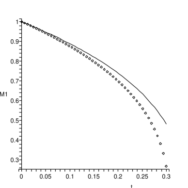
Figure 1: Time evolution of the black hole mass in the commutative case (solid line) compared with the non-commutative case (dotted line). (Normalizations are arbitrary.)

Note that, contrary to the commutative case, the behavior now depends significantly on these parameters. For example, $x_{0}$ should be the detector’s position for the simple case $w=0$ (it appears that one does not learn anything more for $w\not=0$) and one would naturally set $x_{0}\gg 2\,M$, since the detector in the black hole case should stay sufficiently away from the horizon. This will of course damp the non-commutative correction exponentially. Analogously, one may guess that $B\sim 2\,M$ ($\sim 1/T$), since that is the asymptotic position of the mirror (the horizon), and it would then follow that $\kappa\,B$ is just a number which can be simply eliminated by rescaling $\Theta$ (to the same value for all black hole evolutions). However, $A$ represents a transient in the mirror’s trajectory which could be different for different time evolutions, thus allowing to distinguish between different black hole evolutions, and that it enters the final result is a novelty (the standard result does not appear to depend on any transients to leading order in perturbative field theory on the black hole background).

We now calculate the mass of the black hole as a function of time by integrating numerically the previous equation. For the purpose of displaying a result, we arbitrarily set $\tilde{\Theta}=0.1$, and plot the time dependence of the black hole mass in Fig. 1. The graph shows that the black hole life-time is decreased if space-time is non-commutative. Of course, this result bears the same limitations as the original Hawking’s formula, that is, it is unreliable for small black hole mass for which microcanonical corrections become relevant micro .

V Discussion

The form for the mathematical expression for the decay rate of a black hole seems to depend strongly upon the assumptions made. In most cases when a deviation from the approach used by Hawking is made, e.g. assuming the existence of large extra dimensions, microcanonical versus the canonical ensemble micro , or using the Randall-Sundrum brane-world scenario CG , the decay rate of a black hole is reduced compared to that of the Hawking result.

The same conclusion seems to follow from regular black hole solutions regBH , recently (re)discovered in the context of gravity with a minimal length nico which is naturally related to non-commutativity in space-time. The increased decay rate for the case of non-commutative space-time which we found therefore appears to be somewhat unusual. It is possible that the analogy between the black hole and the “kinematical” model of the moving mirror cannot be simply carried on to the non-commutative case, or that what we found “adds” to the sort of effects obtained in the different approaches mentioned above.

Barring the above argument, our result may have interesting cosmological implications for phenomena involving primordial black holes. We do not have a numerical estimate of the decrease in life-time of an evaporating black hole, but the effect will be small since the parameter of non-commutativity $\Theta$ is small in some sense. Nevertheless, primordial black holes evaporating in non-commutative space-time would have to be created at an early stage in the evolution of the universe with an even larger mass than the $10^{15}$ grams required in the commutative case in order to have survived to the present epoch.

References

- (1) N. Seiberg and E. Witten, JHEP 9909, 032 (1999).
- (2) N. Seiberg, L. Susskind, and N. Toumbas, JHEP 0006, 044 (2000).
- (3) J. W. Moffat, Phys. Lett. B491,345 (2000).
- (4) E. Witten, Surveys Diff. Geom. 7, 685 (1999).
- (5) H. S. Snyder, Phys. Rev. 71, 38(1947).
- (6) A. Smailagic and E. Spallucci, J. Phys. A37, 1 (2004).
- (7) A. Smailagic and E. Spallucci, J. Phys. A36, L517 (2003).
- (8) N. D. Birrell and P. C. W. Davies, Quantum Fields in Curved Space, Cambridge University Press, 1982.
- (9) S. W. Hawking, Nature 248, 30 (1974); Comm. Math. Phys. 43, 199 (1975).
- (10) B. Harms and Y. Leblanc, Phys. Rev. D 46, 2334 (1992); R. Casadio and B. Harms, Phys. Rev. D 58, 044014 (1998).
- (11) D. Page, Phys. Rev. D 13, 198 (1976); Phys. Rev. D 16, 2402 (1977).
- (12) R. Casadio and B. Harms, Int. Jour. Mod. Phys. A17, 4635 (2002); R. Casadio and C. Germani, Prog. Theor. Phys. 114, 23 (2005); R. Casadio, Phys. Rev. D 69, 084025 (2004).
- (13) S. A. Hayward, e-Print Archive: gr-qc/0506126.
- (14) P. Nicolini, J. Phys. A38, L631 (2005); P. Nicolini, A. Smailagic, and E. Spallucci, e-Print Archive: hep-th/0507226.