AMR, stability and higher accuracy

Abstract

Efforts to achieve better accuracy in numerical relativity have so far focused either on implementing second order accurate adaptive mesh refinement or on defining higher order accurate differences and update schemes. Here, we argue for the combination, that is a higher order accurate adaptive scheme. This combines the power that adaptive gridding techniques provide to resolve fine scales (in addition to a more efficient use of resources) together with the higher accuracy furnished by higher order schemes when the solution is adequately resolved. To define a convenient higher order adaptive mesh refinement scheme, we discuss a few different modifications of the standard, second order accurate approach of Berger and Oliger. Applying each of these methods to a simple model problem, we find these options have unstable modes. However, a novel approach to dealing with the grid boundaries introduced by the adaptivity appears stable and quite promising for the use of high order operators within an adaptive framework.

I Introduction

There is growing concern in the numerical relativity community about the accuracy that can be achieved as robust implementations of the Einstein equations become available. As has been discussed a number of times, the simulation of strongly gravitating astrophysical systems in 3D requires the stable and accurate handling of a large range of time and length scales lehnerreview ; milleraccuracy . In the context of finite difference schemes, increasing resolution by using more grid points in a uniform grid quickly becomes prohibitively expensive, particularly with multiple spatial dimensions. Two ways of achieving better accuracy include (i) the use of higher order methods for derivative approximations and time integration, and (ii) the use of a grid hierarchy which adapts to provide resolution only where and when needed, so called adaptive mesh refinement (AMR). Both strategies have been adopted by the community largely following two independent paths. On one hand higher derivative operators are being introduced multipatch1 ; multipatch2 ; thornburg ; zlochower ; gioeldave and on the other AMR techniques within a second order accurate implementation have been adopted for over a decade ChoptuikAMR . (For recent efforts implementing second order AMR/FMR see for instance refsAMR /refsFMR )

One key reason behind these independent developments lies in the complications encountered when implementing AMR techniques, especially related to the way the (artificial) interface boundaries are treated. Special care must be taken when dealing with the conditions at these boundaries, in particular how derivative operators should be modified near them. In the case of second order accurate implementations, there is little ambiguity on what these modifications can be as they need only be done at interface points. For higher order implementations, the strategy is far less clear. However, there are strong reasons to combine AMR and implementations of higher orders. For instance, although higher order operators (be they within finite difference, finite elements or spectral approximations) do in principle provide an approximation with errors which are considerably smaller, they do so only if the underlying solution involved is well resolved by the adopted grid. Certainly, the required grid can be anticipated for linear problems but this is hardly the case in non-linear ones where finer features induced by the non-linear nature of the problem can appear during the evolution. Hence, an adaptive gridding mechanism which reacts to the solution itself is crucial. The combination of AMR with higher order operators then provides lower errors for a given grid while being able to react to unanticipated features in the solution —in addition to providing a more efficient use of computational resources—.

In order to combine these techniques, one must face how to treat the derivative operators near boundaries, and how to deal with the artificial boundaries themselves. A clean way to approach this problem is to consider operators satisfying summation by parts (SBP) which have recently been incorporated successfully in strongly/symmetric hyperbolic systems in numerical relativity lsu1 ; lsu2 ; lsu3 ; multipatch1 ; multipatch2 . These techniques guarantee that a large set of problems can be implemented stably.

Having stability of the unigrid evolution, however, is not sufficient to guarantee a fully discrete energy estimate for an AMR implementation. The analysis of the time integration, in particular how different grids communicate with each other to provide boundary conditions, becomes quite involved. Nevertheless, one can argue strongly for adopting as a starting point an implementation in which a semi-discrete estimate is guaranteed since a necessary condition for an AMR implementation to be stable is that its unigrid version be stable. As discussed in the literature, the latter is guaranteed when employing Runge Kutta operators of orders higher than 2 tadmor (in conjunction with suitable boundary conditions).

We thus adopt a strategy where spatial derivative operators satisfying SBP, along with Runge Kutta time integrators, are employed on all levels of the AMR hierarchy. This choice, of course, does not dictate the treatment of the interface boundaries, and we consider various options for this treatment. For instance, in the standard Berger–Oliger strategy, the solution obtained at a parent grid is employed to define boundary conditions for the child grid. Leaving the stability issue aside for a moment, an immediate observation is that when employing a two-level implementation, this strategy can not generically give better accuracy than second order if boundary values are obtained by linear interpolation in time of the parent grid values. Additionally, the definition of all field values via interpolation –without regard for their propagation features– is a likely source of inconsistencies making stability a delicate issue.

In this work we examine alternative treatments of grid boundaries and derivative operators to deal with these issues. We pay particular attention to the stability of the system by effectively implementing a toy model problem within a fixed two-grid hierarchy and analyzing the spectrum of the overall update operator. These studies demonstrate that implementations with accuracy orders greater than two, employing the standard Berger–Oliger scheme have unstable modes. Furthermore, related schemes share this unfortunate feature. This instability can be remedied, with some caveats, with the addition of dissipation though at the expense of larger errors in the approximation. Additionally, we observe that a simple modification of the standard strategy yields a stable scheme without requiring the addition of dissipation, albeit at additional computational cost. In this new strategy, a child grid effectively never requires boundary points from a parent. This can be achieved if the solution at level $n+1$ is obtained by integrating using the past domain of dependence of the child grid only. At first sight this is more computationally demanding as it requires the area of the child grid at level $n$ to be larger than that at $n+1$ so that the intersection of the numerical domain of dependence of the solution at the level $n+1$ is completely contained in the refined region at level $n$. This is achieved simply by defining an ‘extended’ child grid at level $n$ and discarding a buffer zone at level $n+1$. As we will see later in Appendix A, this extra cost need not be relevant at all, as for a given target error, a coarser base grid treated this way might be comparable to a finer base grid treated with the standard Berger–Oliger scheme plus the addition of dissipation.

This work is divided as follows. In Section II, we detail different boundary treatments and describe our method to assess their stability properties. In Section III, we present one and three dimensional tests which illustrate the behavior observed. Section IV concludes with some final comments, and we defer to Appendix A the discussion of the cost associated with 2nd vs. 4th order implementations.

II Technique and stability issues

In searching for a stable AMR implementation, a basic requirement is to have a stable implementation of the equations in the uniform grid case. This requirement is perhaps the most important building block, without which an AMR implementation will suffer even more in terms of stability. Unfortunately, even when ensuring the unigrid scheme is stable, no results are available on what guarantees the stability of an AMR/FMR implementation with ‘sub-cycling’ for arbitrary accuracy orders. Such a scheme which advances a grid with a time step defined by its grid spacing stands in contrast to one which advances all points by a global time step determined by the finest resolution in use. The latter is considerably less efficient than the former (becoming more so with more refinement levels) but is simpler to analyze. We concentrate here on the former case, i.e. one that involves sub-cycling, as this is the method one would like to employ.

In order to develop a stable AMR/FMR scheme, we analyze different natural options from their fully-discrete point of view and study their stability properties. We begin by adopting a strategy that ensures stability for a uniform grid case for first order (non-constant coefficient) symmetric hyperbolic linear systems. This strategy calls for employing derivative operators satisfying “summation by parts” (SBP) together with an appropriate time integrator such as 3rd/4th order Runge–Kutta schemestadmor . The first ingredient allows one to derive a semidiscrete energy estimate while the second one guarantees this estimate will be preserved in the fully discrete case. Following this strategy, we employ such operators here as our main building blocks; as mentioned above, they provide a strong platform for developing a useful AMR/FMR prescription.

Having defined the constituents of the basic update routine, we now turn our attention to the creation and update of a child grid and how updated field values on this grid are to affect those in the parent one. Our goal is to obtain a recipe that will allow us to distinguish among different possibilities, the ones that guarantee stability for a simple model problem. As we will show, even when applied to a simple model problem, the analysis we present does well at predicting either stability or instability, suggesting applicability for more general problems. Although our analysis applies to a simple model problem, the scheme it reveals to be stable is one that will naturally yield a stable scheme if it is so for a unigrid implementation. Since the adoption of operators satisfying SBP together with an appropriate Runge–Kutta update scheme guarantees stability for generic non-constant coefficients first order linear systemslsu1 ; lsu2 , the higher order AMR scheme will preserve this property.

To fix ideas and to simplify the presentation of our analysis, we restrict to the case where second and fourth order accurate schemes are employed. This is sufficient to illustrate the salient aspects of the analysis and main results; the conclusion can be trivially extended to arbitrary orders of accuracy.

Analytical Considerations

In order to explore different possible ways to implement an AMR strategy we analyze what a full discrete step involves for the simple equation

$$\partial_{t}u=\partial_{x}u,$$ (1)

on the region $x\in[0,1]$ with periodic boundary conditions, and where a refined region (the child grid) is included within this domain. This can be assumed without loss of generality as the operators employed (satisfying SBP) and a suitable Runge Kutta time update (together with suitable boundary conditions) guarantee the stability of the implementation. Thus, to avoid unnecessary clutter in the analysis we examine the periodic case for the coarsest grid involved. For simplicity, we restrict ourselves to the case of fixed mesh refinement with the child grid $2:1$ refined with respect to the parent grid. We then compute the eigenvalues of the full amplification matrix ($Q$) corresponding to the update scheme of field values on the parent level. Clearly, if all the absolute values of this matrix are bounded by unity, amplification at each step is bounded by one (i.e. modes are either kept constant or damped) and stability follows for the problem under consideration if the matrix can be diagonalized. On the other hand, if there is an eigenvalue with absolute value larger than unity, the amplification per step is unbounded and the algorithm is therefore unstable. Since this applies already to the simplest first order problem, the conclusion that the system is unstable will naturally hold for generic ones. Note that it is sufficient to consider a single refinement level (and the corresponding coarse grid) in this analysis, as in a generic case consisting of several child grids the total amplification matrix will be a composition of several $Q$ matrices.

The specific form of $Q$ depends on several different ingredients. The cleanest way to construct $Q$ is to express it as a composition of different matrices, each representing the action of an operator performing a specific task involved in the overall update strategy. For the problem under consideration, we need to consider the matrices

• $J_{21}$ which defines the grid values on the child level by knowing those at the coarse level, usually referred to as prolongation or interpolation.

• $D_{1}$ and $D_{2}$ the derivative operators used on the parent and child grids respectively.

• $U$, the specific time stepping algorithm.

• $J_{12}$ which restricts the values obtained on the child grid at the new coarse time level at appropriate points of the coarse grid; usually referred to as restriction or injection.

• $R$ a restriction operator which, when acting on an overall update scheme, restricts its values to the region in the coarse grid which needs no refinement. Hence, $1-R$ restricts the action of any operator to the points in the coarse level which do require refinement.

• $B$, boundary points definition at intermediate child grid time levels which, depending on the strategy adopted, one might have to consider.

An update step in a two-level scheme which takes values on the $n$-th level of the coarse grid ($u_{c}^{n}$) and yields values at the $n+1$-th level ($u_{c}^{n+1}$) can be expressed as $u_{c}^{n+1}=Q_{c}u_{c}^{n}$, with:

$$Q_{c}\equiv RU_{c}+(1-R)J_{12}\,U_{f}\,J_{21},$$ (2)

with $U_{c}$ and $U_{f}$ the update steps on the parent and child grids. For instance, for the advection equation above, and employing a 3rd order Runge Kutta scheme, $U_{c}$ becomes (for a periodic boundary problem)

$$U_{c}=1+\Delta tD_{1}+\frac{(\Delta t)^{2}}{2}D_{1}^{2}+\frac{(\Delta t)^{3}}{6}D_{1}^{3}.$$ (3)

The expression for $U_{f}$ is more delicate and depends crucially on the scheme adopted. For instance, when employing $2nd$ order derivative operators, and the standard Berger-Oliger strategy for treating interface boundaries, one schematically has

$$T^{n}_{1} = B\left(1+\frac{\Delta t}{2}D_{1}\right)+(1-B)\,I_{n+1/4}\,,$$ (4)

$$T^{n}_{2} = B\left(1+\frac{3\Delta t}{4}D_{1}T^{n}_{1}\right)+(1-B)\,I_{n+3/8}\,,$$ (5)

$$T^{n}_{3} = B\left(1+\frac{\Delta t}{9}(2D_{1}+3D_{1}T^{n}_{1}+4D_{1}T^{n}_{2})\right)+(1-B)\,I_{n+1/2}\,;$$ (6)

$$Q_{f} = T^{n+1/2}_{3}T^{n}_{3},$$ (7)

with $T_{i}$ denoting the intermediate steps of the Runge-Kutta algorithm, $B$ the identity operator at the interior points of the child grid, but zero at interface boundaries; $I_{m}$ the interpolation of field values at points on the coarse grid (at interface boundary points) providing values at the $m$-th time level required by the time stepping algorithm.

The above is just an example of what a typical procedure entails as there certainly are many alternatives for the injection/prolongation, update, derivatives operators and boundary definition that will be part of the AMR/FMR strategy. A partial restriction is introduced when choosing the accuracy order desired as this fixes the derivative operators at interior points (by adopting the standard centered operators). However this still leaves considerable freedom related to the way derivatives are to be defined at points at, and close to, the boundaries, in addition to the definition of the interpolating operators $I$ to be used (if so desired) in defining interface boundary points, the injection and prolongation operators, etc. The analytical investigation of every option is an involved task. To reduce the number of possibilities we adopt some simplifying, yet natural and commonly used, assumptions. Throughout this work we concentrate on two-level schemes. We consider interpolating operators acting only at interface boundary points and, at most, a few additional points at each side of the refined grid. As much as possible we adopt the same basic integration step for all grids to ensure that a recursive type algorithm can be easily employed. Finally we concentrate on vertex-centered schemes and child grids having points lying on a coarse grid points. Even with these simplifications, obtaining the eigenvalues of the amplification matrix is a cumbersome task. For this reason, we perform our investigations with the aid of a computer algebra package (Maple) to numerically calculate the eigenvalues.

To do this, we define a grid composed of $N_{1}$ points describing the coarse level and where $M<N_{1}$ points will be refined (the child grid has $N_{2}=2M+1$ points). We construct the matrices defined above, obtain the amplification matrix and numerically calculate the eigenvalues. Since we perform these calculations for a fixed number of grid points (though we have varied $N_{1}$ and $M$ over several values), a negative result (all absolute values less or equal than unity) does not constitute a stability proof, but certainly a positive result, (at least one eigenvalue with larger than unity absolute value) shows that the proposed algorithm is unstable. We can thus substantially narrow the search for likely stable ones and the tests considered in Section III lend additional strength to our analysis. As we will see, our analysis indicates a preferred option which, intuition suggests, will be stable for any problem where the unigrid case is stable.

The construction of the amplification matrix proceeds in the following way. First a whole time step is taken in the coarser grid, so that we can use, if so desired, the values at the next time step to impose boundary conditions for the intermediate time steps taken on the finer grid. Once the recipe to provide these boundary conditions is given and the difference operator on the finer grids chosen, the algorithm is pretty much fixed. Other alternatives include not providing boundary conditions at all but rather to taper off the child grid as subsequent intermediate child time levels are obtained. Additionally, one might consider other variants at the level of the interpolation order on $J_{21}$, a possible averaging at the injection level, $J_{12}$, or at the coarser grid, etc. We analyzed several of these options and report on their results in the following subsections.

Finally, as mentioned, we limit ourselves to Runge-Kutta time integrators of order larger than two as these are known to lead to stable schemes if the semi-discrete system is stable tadmor .

II.0.1 Second Order Schemes

Here we use a third order Runge-Kutta time integrator (RK3) as the second-order Runge-Kutta method is not known to guarantee the fully-discrete stable scheme if the semi-discrete scheme is stable. The population of the finer grid, given by the operator $J_{21}$, is carried out using four-point stencil interpolation (having an $O(h^{4})$ error) on the child grid points lying in between coarse ones and using a direct copy of field values where the grid points coincide (see appendix B for the interpolator’s specific form). We consider the following cases:

• Berger Oliger: (berger2 ) Here we reproduce the “standard” Berger-Oliger scheme and check its stability when used with RK3. Figure 1 illustrates the points involved in this scheme. Here the values at the diamond points, needed for the intermediate RK steps of the finer grid (squares), are obtained via linear interpolation in time employing values at the top and bottom points of the coarse grid (circles). The coarse grid points are already known at the advanced time step because it takes a full time step before the fine grid is advanced. The dotted lines represent the RK steps intermediate to a full time step of the child grid. On the fine grid, only the square points are evolved, using centered difference operators, and at the end of the cycle the values of the fine grid coincident with coarser points are directly injected into the corresponding coarse grid points.

  Figure 1: Standard Berger Oliger Scheme. Circles/squares denote coarse/fine grid points while diamonds denote boundary points at which values are filled via interpolation from the coarse grid.

• Penalty Method: In this case, in contrast to the previous one, we pay close attention to the propagation modes defined by the equation of motion. In this simple case, the single characteristic propagates from right to left (see Figure 2). Thus, only boundary values at the right end of the fine grid are required. These are provided by linearly interpolating coarse field values at the top and bottom levels and used as boundary conditions in a scheme enforcing these via penalty terms as described in carpenter0 ; carpenter1 ; multipatch1 . In this technique, boundary values are incorporated by modifying slightly the right hand side of the (first order) equations. For our test problem this results in

  $$Du\rightarrow Du+P\kappa\frac{1+\delta}{dx}(u_{b}-u)\,,$$ (8)

  where $D$ is the discrete derivative operator (satisfying SBP) employed; $P=0$ for $i=1..N-1$ and $P=1$ at $i=N$ (i.e. only non-zero at the right interface boundary point); $\delta$ is a free parameter and $\kappa$ is related to the norm/derivative operator employed in ensuring SBP is satisfied (see multipatch1 for a detailed description).

  The penalty technique provides a clean and efficient method to provide boundary values which, coupled with the use of operators satisfying SBP, guarantees the stability of the implementation. Furthermore, within this approach, all points are updated and the boundary conditions are imposed via a simple addition of suitable penalty terms to the right hand side at boundary points. For these reasons it represents, at first sight, a convenient approach to handle characteristic modes within an AMR/FMR implementation. As with the Berger-Oliger scheme, after the child grid update to the same time as the parent, field values coincident with the parent are directly copied.

  Figure 2: Penalty Scheme. Circles/squares denote coarse/fine grid points while diamonds denote boundary points at which values are filled via interpolation from the coarse grid. Notice only the points at the right are defined this way as the system describes modes propagating from right to left.

• Tapered Boundary Method: In this case, we adopt restriction operators which effectively remove points that have been influenced by the interface boundary. In practical terms, this means that if the child grid at the advanced $n+1$ level is defined as $\{x\in[L,R]\}$, the update from level $n$ must take place in the region $\{x\in[L-\triangle,R+\triangle]\}$ with $\triangle\equiv n_{p}dx$ given by a sufficient number of points to insure that the numerical domain of dependence of $[L,R]$ starting at $n+1$ is completely contained in $[L-\triangle,R+\triangle]$. This is illustrated in Fig 3. The size of $\triangle$ is determined by the order of accuracy of the discrete operators involved and the maximum speed of the hyperbolic problem considered.

  Incidentally, note that this is not the same as an alternative approach where ghost zones populating a region around the refined region (with values obtained via linear interpolation from the coarse values at levels $n$ and $n+1$) are defined. That approach is relatively straightforward to implement and reduces the complexity of the derivative operators employed, but does not satisfy the requirement that what is done at the boundary has no influence on the final injected point. As we will see later, this scheme also has unstable modes.

  Figure 3: Tapered Scheme. Empty circles/squares denote coarse/fine grid points while filled squares schematically indicate those belonging to the fine grid which are affected by the presence of the boundary (either by derivatives at these being different from the centered one, and/or that their update reaches up to these points). Dashed lines indicate the past domain of dependence of the refined region at level $n+1$ and its intersection with level $n$ indicates the region that needs to have values in the fine grid. Hence, all fine grid points outside the domain of dependence are effectively discarded.

2nd order schemes: Summary of results and observations

The analysis of the eigenvalues of the amplification matrices corresponding to each of the three cases discussed above must be examined carefully as we are considering the fully discrete case. Here a competition among the unstable modes and the possible inherent dissipation of the update scheme determines whether the eigenvalues’ magnitude of the full amplification matrix are indeed larger than unity. In particular, for large CFL values, the inherent dissipation grows and the eigenvalues might be bounded by unity while for smaller CFL values this might not be the case. As we are interested in establishing stability with at most an upper bound for the CFL value we have examined several possible values of CFL (ranging from $1$ to $10^{-4}$) and observe when unstable modes arise. For instance, for a CFL value of $1$ all eigenvalues for the three approaches lie within the unit circle as illustrated in Fig. 4. However, as this value is decreased unstable modes do appear for the penalty case while not for the other two options. One can exploit the free parameter $\delta$ to alleviate the instabilities in the penalty case (in the sense that the magnitude of the eigenvalues gets closer to unity) but not completely remove them with the addition of artificial dissipation.

Additionally, it is instructive to investigate the behavior of the error as a function of position to obtain some indication of the effect the artificial boundaries have. To this end, we compute the error in the evolution of $u(t=0,x)=\sin(\pi x)$ after a single step for each case. Here the solution after a step is $u(t=h,x)=\sin(\pi(x+h))$ and a point-wise error calculation is straightforward to compute. The results are indicated in Fig. 5. The differences in the errors among the three schemes are clear. The B-O and tapered approaches have similar errors while those of the penalty scheme are larger due to the derivatives at the boundaries being calculated to first order accuracy.

Figure 4: Stability region of the fully discrete step for the Berger-Oliger, penalty and tapered schemes (from left to right respectively). For a CFL=1, all eigenvalues corresponding to each of the amplification matrices lie within the unit circle.

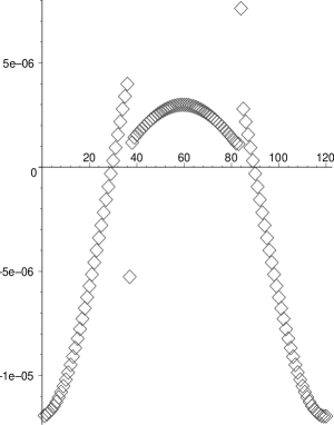
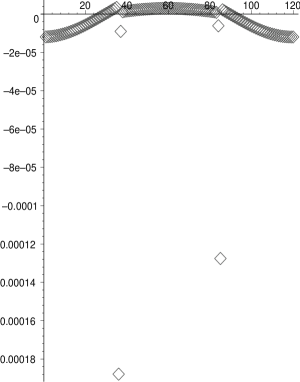
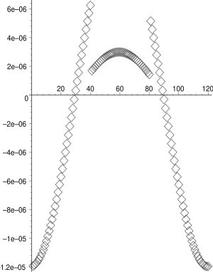
Figure 5: Measured errors after one full step in the evolution of $u=\sin(\pi x)$ in the domain $[0,1]$ under the three schemes considered —from left to right: the B-O, penalty and tapered schemes—. A CFL factor of 0.25 was employed and no artificial dissipation added.

II.0.2 Fourth Order Schemes

Here we use a fourth order Runge-Kutta time integrator and analyze the stability properties of the obtained schemes under the cases considered above. In this case, we will find that only the tapered boundary approach yields a stable scheme unless a carefully tuned amount of dissipation is added to the problem. We have found the same holds true when adopting a third order Runge-Kutta operator.

We adopt fourth order accurate centered difference operators (in the case of Berger-Oliger type schemes) or those satisfying the SBP property, in the case of the penalty approach. For the tapered boundary approach it does not matter which one is employed as points affected by ‘special’ boundary treatments are to be discarded.

The population of child grid points lying between coarse ones uses a six-point stencil interpolation operator (having an error of $O(h^{6})$) to ensure that the discontinuity in the truncation error in between different grids does not affect the order of the scheme (see appendix B for the specific expressions of the interpolators). For a first order equation, employing fourth order derivative operators requires at least a fifth order interpolation stencil. We adopt sixth order to avoid spoiling the symmetry of the implementation.

We consider the following cases:

• Berger-Oliger Method:

  Here the setting is as in the second order case, but some modifications must be introduced at the level of the derivative operators employed. One option is to modify them near the boundaries in a side-ways manner so as to preserve the order of the approximation. The other is to define extra ghost zones around the refined region and keep the derivative operator in its standard centered expression. We have analyzed both cases with similar qualitative results. We discuss here the latter case in some detail.

  For a fourth order accurate approximation to the derivative operator only two ghost zones on each side of the grid are needed. One is located at the interface boundary while the other is placed next to it outside of the refined region. As before, the field values at these points are to be defined via interpolation from those known at the coarse level on levels $n$ and $n+1$. We examined both linear interpolation –with error $O(h^{2})$– and quadratic interpolation –with error $O(h^{3})$– . The latter option employs the value of the field at the $n$ and $n+1$ level (as in the linear case) together with the time derivative of the fields at level $n$. The qualitative features of the amplification matrix is the same in both cases, namely that there exists eigenvalues with magnitude greater than one. We did not go beyond this order as it would involve taking further derivatives of the right hand side, which in a general case would involve derivatives of both coefficients and variables

• Penalty Method: Here again the setting is similar to the second order one, the only difference is that at the boundary the interpolation is done at third order, again using the computed right-hand-side of the equations at the initial time. This is only needed at boundaries where there are incoming characteristics as at the other boundaries field values will be defined solely by the update within the child grid itself. Additionally, no extra ghost zones are required as one must use SBP operators of the appropriate order (see for instance, multipatch1 ).

• Tapered Boundary Method: This case is analogous to the second order case. The only significant difference is the size of $\Delta$, which must be enlarged so as to ensure the intersection of the past domain of dependence of the region of interest at the $n+1$ level is completely contained inside the refined region at level $n$.

4th order schemes: Summary of results and observations

The analysis of the eigenvalues of the amplification matrices corresponding to each of the three cases discussed above reveals that there exists eigenvalues with magnitude larger than unity for the B-O and Penalty approaches while none for the tapered one. Clearly the stability of the tapered approach follows from the stability of the unigrid problem. Here again, the amount by which the eigenvalues of the B-O and Penalty approaches are above unity is not too large and depends strongly on the CFL factor employed. However, from our analysis it is expected that as the base grid is refined and smaller CFL factors are used (or a larger number of refinement levels are employed) instabilities associated with these modes will appear. Beyond this point however, the tapered approach also yields evolutions with much smaller errors. To illustrate this we again compute the error in the evolution of $u(t=0,x)=\sin(\pi x)$. The results are indicated in figure 6; again, the effects of the boundaries can be clearly appreciated but this time the errors in the tapered grid are 40 times smaller.

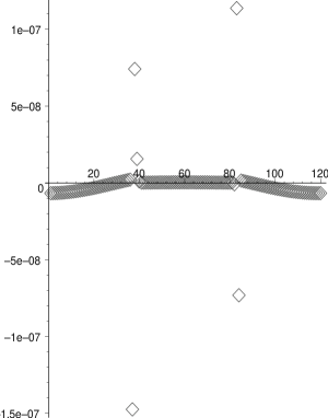
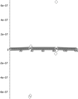
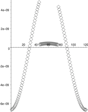
Figure 6: Measured errors after one full step in the evolution of $u=\sin(\pi x)$ in the domain $[0,1]$ under the three schemes considered —from left to right: the B-O, penalty and tapered schemes—. A CFL factor of 0.25 was employed and no artificial dissipation added.

These results make it clear that straight forward extensions of Berger-Oliger to higher order, as well as the use of a penalty method which takes into account the characteristic structure of the problem, suffer from unstable modes in a higher order AMR/FMR scheme. The only option we have found to be free of this problem is that given by the tapered boundary approach, which a priori would appear more computationally demanding as points are evolved which will be discarded. For sufficiently high order schemes, this can be a significant fraction of the grid.

Although this extra cost might not be as significant as it appears (see Appendix A), one might prefer to maintain the standard Berger-Oliger prescription and deal with the unstable modes by introducing some amount of dissipation. Therefore we revisit the analysis above but now with the addition of dissipation. To anticipate the results obtained, we indeed find that dissipation can control the unstable modes but at the expense of increasing the overall error and needing to fine tune it to ensure a desired degree of smoothness in the solution.

II.0.3 Dissipation on Fourth Order Schemes

As noted, the update scheme obtained for the BO and Penalty schemes are unstable for the higher order case; this can be remedied or alleviated by the introduction of some amount of dissipation. We consider the addition in two ways, one as a dissipative operator modifying the right hand side of the equation (and hence involved in all time levels), or as a high-pass filter only at parent levels. The latter is amenable to be analyzed through the method outlined in Section II while the same for the former becomes too cumbersome. The analysis with the addition of the filter shows that the addition of dissipation can render the scheme stable and experimental tests (in the tests presented in the next section) indicates the same holds true with the first option. Here we present results of the errors obtained after a single step in each of the approaches considered, illustrated in figures 7 and 8. These figures show the errors obtained after a single evolution step of a (well resolved) smooth initial data given by $u=\sin(\pi x)$. Figure 7 displays the observed behavior when no dissipation is employed. The errors obtained with the B-O and Penalty approaches are about two orders of magnitude above those seen when employing the tapered approach after a single step. The addition of dissipation alleviates this issue though the amount of the dissipation has to be tuned to yield smooth errors while not affecting their magnitude. Figure 8 show the obtained behavior with $\sigma=0.1$ which is not yet enough to give smooth errors for the B-O approach and even less for the Penalty method while quite suitable for the tapered approach.

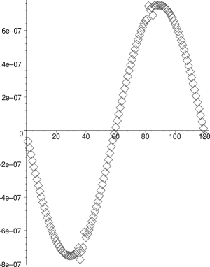
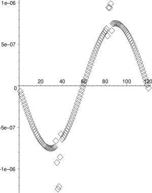
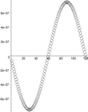
Figure 7: Measured errors after one full step in the evolution of $u=\sin(\pi x)$ in the domain $[0,1]$ under the three schemes considered —from left to right: the B-O, penalty and tapered schemes—. A CFL factor of 0.25 was employed and artificial dissipation of the Kreiss-Oliger form has been added with $\sigma=0.1$. This value of $\sigma$ is not yet enough to smooth-out the errors in the B-O and Penalty approaches, though in the first case makes the errors about the same as those obtained with the tapered approach.

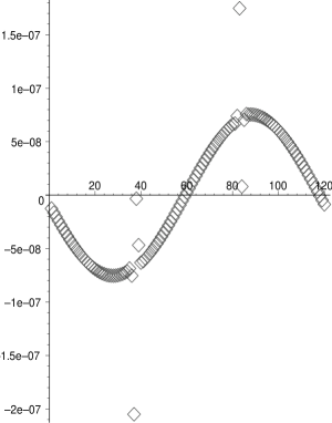
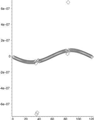
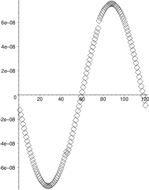
Figure 8: Measured errors after one full step in the evolution of $u=\sin(\pi x)$ in the domain $[0,1]$ under the three schemes considered —from left to right: the B-O, penalty and tapered schemes—. A CFL factor of 0.25 was employed and artificial dissipation Kreiss-Oliger type dissipation has been added with $\sigma=0.01$. This value of $\sigma$ is too small to smooth-out the errors in the B-O and Penalty approaches while is still reasonable for the tapered approach. Furthermore, the errors in the B-0 approach are now about $4$ times larger than in the tapered one.

III TESTS

In the following one-dimensional series of tests, we consider four natural alternatives. These differ in their handling of refinement boundaries, in particular how they compute derivatives there and what conditions are imposed. Derivatives at interior points are defined by the standard centered ones.

These alternatives are: (I) sideways derivatives (constructed so that their approximation order is equal to that of the centered derivative operator employed at the interior points); (II) derivatives of lower order near the boundaries, which, in the absence of a time interpolation, would satisfy summation by parts; (III) Centered derivatives throughout, with extra ghost zones on each side of the child grid as needed for applying the standard centered derivative. In the above three cases, boundary (and guard) data as the integration proceeds is obtained via interpolation from the parent grid. The last option (IV) is the “tapered boundary approach” described in Section II.0.1.

III.1 Numerical Results. 1D tests

We study the long term evolution of several systems implementing an FMR scheme. Since in this case the grid-structure is fixed it does not correspond to a well suited adaptive simulation, as the adaptivity would sequentially create grids to follow the traveling features in the solution (assuming, of course, an appropriately defined refinement criterion is in place). However, this arrangement is well suited for our task here to assess the stability of the simulation and the interaction of features in the solution propagating in and out of the finer refined regions.

Our tests consist of:

• The first test is restricted to the simplest possible case provided by the advection equation $u_{,t}=u_{,x}$. This is a hyperbolic system with constant in time and space coefficients. For such a simple case, it is observed that higher order accuracy can be achieved with a rather simple interface boundary treatment.

• The second test corresponds to a linearization of the Einstein equations with respect to a time/space dependent background.

• The last test corresponds to the full Einstein equations restricted to a spherically symmetric case. In this case, excision techniques are also implemented.

III.1.1 Advection equation

We here concentrate on the advection equation $u_{,t}=u_{,x}$ discretized in the domain $L_{0}=\{x\in[-2,2]\}$ with two levels of refinement $\{L_{1},L_{2}\}$ given by $L_{n}=\{x\in[-1/n,1/n]\}$ ($n=1,2$). Periodic boundary conditions in the $L_{0}$ grid are enforced directly at the difference operators level while interface boundaries $x=\pm 1/n$ are handled via the standard B-O method or the tapered boundary approach. We implemented both second and fourth order accurate derivative operators with a fourth order Runge Kutta operator for the time integration. The initial data is given by a compact support pulse given by

$$u(t=0,x)=\left\{\begin{array}[]{ll}\kappa(x/L-1)^{5}(x/R-1)^{5}&\mbox{if $x\in[L,R]$}\\ 0&\mbox{otherwise \, ,}\end{array}\right.$$ (11)

with $\kappa=30$, $L=-0.55$ and $R=0.95$. These limits are arbitrarily defined ensuring the pulse lies in the middle grid. As time progresses, the pulse will move across all grids.

For the second order case, we have seen that all options discussed give a stable implementation. We corroborated this by monitoring the error in the solution obtained with both the BO and Tapered boundary approaches. To this end, we evolved the solution on a uniform grid with $1601$ points and adopted it as our “analytical solution” $F_{a}$ (recall that the unigrid problem is guaranteed to be stable). We then run with both implementations using a coarse grid consisting of $101,201$ and $401$ points and calculate the error for each numerical solution $F_{n}$ as $E_{n}\equiv F_{n}-F_{a}$. Figure 9 illustrates the observed behavior which indicates both approaches give practically the same solutions. Next we calculate the convergence rate with these obtaining values consistent with second order accuracy as shown in figure 10.

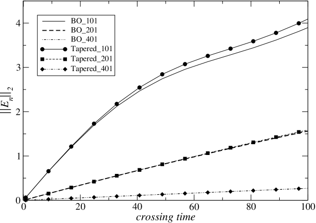
Figure 9: Errors in the $L_{2}$ norm of the solution obtained with the B-O and tapered boundary approaches. A CFL $=1$ was employed and no dissipation. Note that the vertical axis has not been rescaled the error in the solution indeed becomes very large after several crossing times manifested in large phase/amplitude errors.

.

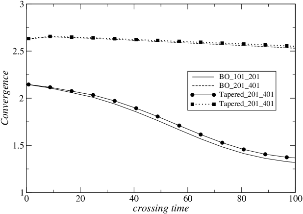
Figure 10: Convergence rates measured for both cases obtaining similar results.

.

When employing fourth order accurate derivative operators as discussed in Section II.0.2, boundary conditions are required in approaches (I) through (III). We consider both linear and cubic interpolation employing in the first case the values of the function at the coarser time levels and in the second case we include the time derivative to obtain a cubical interpolant. These interpolations provide boundary data at points $x=\pm 1/n$ and $x=\pm(1/n-1/(n(N_{c}-1)))$. Notice that when employing cubical interpolation in time and linear interpolation in space, no significant qualitative differences were observed if a higher order interpolation in space was employed.

As discussed previously, without the addition of dissipation, options (I) through (III) yield unstable implementations, and we have confirmed this by monitoring the $L_{2}$ norm of the solution vs. time. By running for several crossing times for different resolutions, it is seen that the norm grows faster for finer refined grids. Next, in order to control to some extent the instability, we add dissipation to the problem. This can be done in two forms, one is by modifying the right hand side of the equations by introducing a dissipative term and the other is to apply a filter to the updated variables. In the second option the filter applied is, in a sense, equivalent to introducing an integration on a fictitious time after each step (with respect to the coarsest grid) of the equation $u_{,t}=\sigma d^{3}\partial_{xxxx}u$. This results in the replacement

$$u^{n}_{i}\rightarrow u^{n}_{i}+\sigma\left(6u^{n}_{i}-4(u^{n}_{i+1}+u^{n}_{i-1})+u^{n}_{i+2}+u^{n}_{i-2}\right).$$ (12)

As a comparison of what is observed, figure 11 illustrates the the $L_{2}$ norm of the difference between the solution obtained with $N$ and $2N$ points vs. time (with $N=100,200$). The figure illustrates the behavior of this quantity for the solutions obtained with the B-O approach obtained with two different dissipation and CFL parameters. These solutions are obtained with strategy III (namely with two ghost zones on each side of the child grids to employ the standard centered difference operator). We additionally show the corresponding result for the tapered boundary approach. As illustrated in the figure, while the dissipation manages to control the exponential growth of the solution, convergence is severely affected. The solution obtained with the tapered boundary approach on the other hand, behaves stably and the error scales as expected. Figure 12 shows the convergence factors calculated with these solutions, while the tapered boundary approach yields a value quite close to the expected one of $4$, the one obtained with strategy III quickly deteriorates.

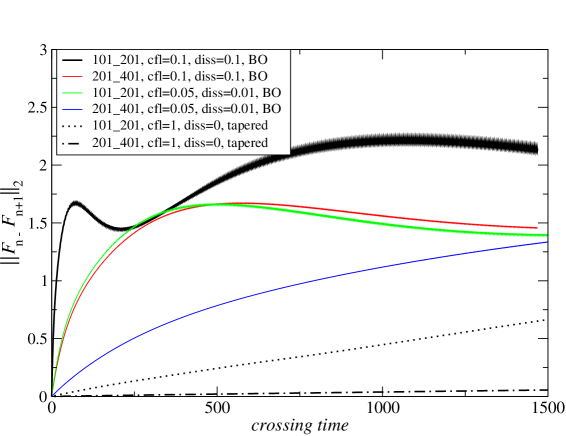
Figure 11: Differences in the solutions obtained with different CFL/dissipation combinations

.

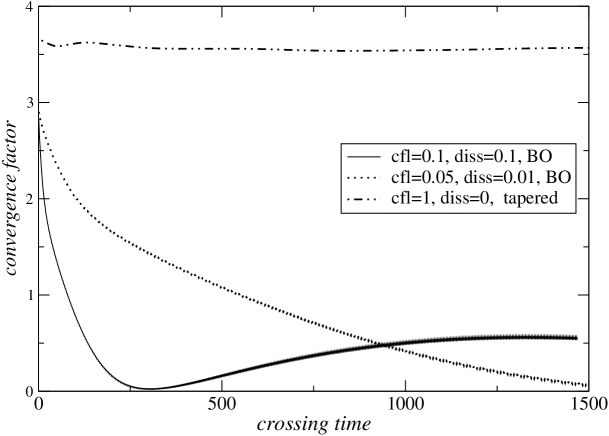
Figure 12: Convergence factors obtained when employing different CFL/dissipation combinations

.

Finally, as was discussed in Section II.0.2, unless both the CFL and dissipation parameter are chosen carefully, this filtering might not be enough to control the instability. For instance, for a CFL factor $=1$ and $\sigma=-0.05$, the growth of the instability is less severe and might not be visible for relatively coarse resolutions for long times though as the grid is refined the instability might become evident. We illustrate this behavior, and contrast it with the one observed with the tapered grid approach, by monitoring the $L_{2}$ norm of the error $E_{n}$ defined as in the second order case (i.e. with respect to the solution obtained with a unigrid evolution on a grid consisting of $3201$ points). Figure 13 shows the results obtained for the coarse grids having $101$ and $401$ points. Clearly, while the tapered boundary approach gives the expected behavior, strategy (III) with the addition of dissipation fails to give good answers. Notice that while the solution obtained with $101$ points does not exhibit an instability the one with $401$ points does so clearly. The reason behind this is that the instability for the coarser case has not yet grown above the truncation error in the solution.

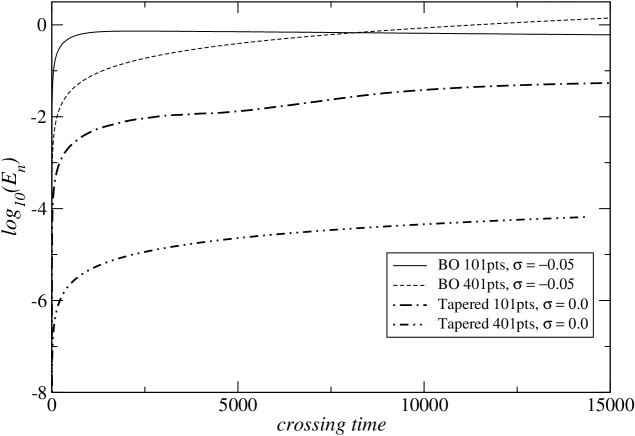
Figure 13: Errors in the $L_{2}$ norm of the solution obtained with the B-O and tapered boundary approaches. A CFL $=1$ was employed and $\sigma=-0.05$ in the B-O case.

.

III.1.2 Linearized Einstein equations

The second test is defined by considering the linearized Einstein equations off the “gauge-wave” solution. This solution describes flat-spacetime in a coordinate system that introduces an explicit time-position dependence of the metric as

$$ds^{2}=e^{A\sin(\pi(x-t))}(-dt^{2}+dx^{2})+dy^{2}+dz^{2}$$ (13)

We then write the linearized Einstein equations off this spacetime in a first order symmetric hyperbolic form as discussed in multipatch1 following the formulation introduced in sarbachtiglio which includes a dynamical lapse. By restricting to perturbations in the $t,x$ directions, solely depending on these coordinates, one obtains a reduced system of non-trivial equations for $\delta g_{xx},\delta K_{xx},\delta d_{xxx},\delta\alpha,\delta A_{x}$. We solve the resulting equations in the domain $x\in[-1,1]$, with $A=0.1$ and compare the results obtained with 2nd and 4th order accurate spatial derivative operators while maintaining $4th$ order accurate integration in time via a Runge Kutta algorithm.

We first run a series of tests employing a $2nd$ order accurate spatial derivative operators, a 4th order interpolation to create child grids, a $4th$ order Runge-Kutta time integrator and a direct injection from child to parent grid points. We concentrate on the accuracy and convergence rate observed for cases (I-III) and (IV) above. Ie, in the first case we employ second order derivative operators at interior points while first order one at the boundaries. Since boundary points in this case are over-written by the time-interpolation cases (I-III) are identical. For case (IV) however, we define extra child points via interpolation from parent to child at level $n-th$. These extra points are discarded at the $n+1th$ level and are solely used to remove any dependence on the refinement boundaries that child points, at the region of interest, have at the $n-th$ level.

First we confirmed that the unigrid code is stable and convergent, and pick the solution obtained with the highest resolution (corresponding to a grid with 3201 points) and consider it the ‘analytically’ expected solution $F_{a}$ which we use to compare the results obtained when using fixed mesh refinement. For these tests we employ a base grid of $101$ and $201$ points, each with 2 levels of refinement (with boundaries at $[-1/q,1/q]$ with $q=2,4$) and no dissipation is included. Figure 14 illustrates the (log of the) $L_{2}$ norm of the difference between the solution obtained at the base grid $F_{n}$ and $F_{a}$ with $n=101,201$. The obtained results with the standard FMR approach and the tapered boundary one are practically indistinguishable from each other. This also implies the convergence of both should be practically the same, ie. second order, a fact that is shown in figure 15.

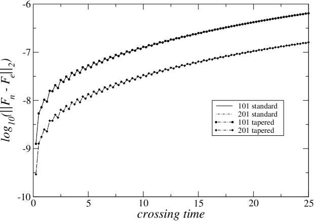
Figure 14: Errors associated with cases (I-III) and (IV) as a function of time. The lines are indistinguishable from each other.

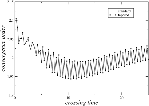
Figure 15: Measured convergence rate for the different methods. There is no appreciable difference in the 2nd order case. Again, there is no appreciable difference with the values obtained with both approaches.

.

In the $4th$ order accurate case, as expected from the analysis presented in section II, differences do arise. For these tests we employ 4th order derivative operators at interior points –suitably modified near the boundaries to cover cases (I) and (II) or ghost zone points suitable added for case (III)–; a 6th order interpolation from parent points to define child grid points; a 4th order RK time integrator and a direct injection from child to parent grid points. As before, we first run a series of unigrid tests to confirm that a stable evolution is obtained as expected and choose the solution obtained with the highest resolution run (obtained with a grid consisting of 3201 points) and consider it the ‘analytically’ expected solution $F_{a}$. Again we consider a base grid of $101$ and $201$ points, each with 2 levels of refinement (with boundaries at $[-1/q,1/q]$ with $q=2,4$) and as above no dissipation is included.

Figure 16 illustrates the (log of the) $L_{2}$ norm of the difference between the “analytical” solution and those obtained with a coarse grid (plus the two refinement level) $F_{n}$ with $n=101,201$. Clearly the errors associated with the implementations (I-III) grow considerably faster (indeed exponentially) than those obtained with the tapered boundary approach (linearly). In fact, after about $50$ crossing times the error associated with the tapered boundary approach using $101$ base points is approximately the same as that with the standard approach but with a base grid of $201$ points. Figure 17 illustrate the measured order of convergence for these methods, while the value obtained with the “standard approaches” significantly reduces as time proceeds the corresponding one to the tapered boundary approach remains near $4$ decreasing just slightly as errors accumulate over time.

Figure 16: Errors associated with the 4th order accurate approaches. The errors associated to the cases where time interpolation is employed grows exponentially fast while those measured in the tapered boundary approach do so linearly.

.

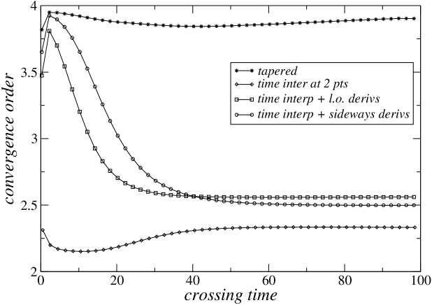
Figure 17: Measured convergence rate for the different cases, while the tapered boundary approach remains close to 4 over 100 crossing times, the convergence of the other methods fall sharply.

.

Last, for illustrative purposes, we show in figure 18 the errors associated with the different solutions obtained with the tapered boundary approach for $2nd$ and $4th$ order accurate spatial operators. The accuracy gained by employing a higher order operator is evident.

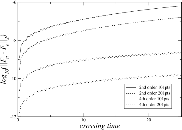
Figure 18: Errors associated with the 2nd and 4th order tapered boundary approaches.

.

III.1.3 Spherically symmetric spacetime

In the last one-dimensional test we consider Einstein equations restricted to spherically symmetric spacetimes in vacuum. The solution for a black hole initial data must be static and hence field variables have only non-trivial radial dependence.

We again employ a grid structure composed of a base grid given by $L_{0}=\{r\in[M,11M]\}$ with two levels of refinement $\{L_{1},L_{2}\}$ given by $L_{n}=\{r\in[M,11/(2n)M]\}$ ($n=1,2$). Thus, while the boundaries at the right boundaries of each domain are sequentially located at smaller radii, the left boundaries all coincide at $r=M$. At these boundaries, for the tapered-boundary approach one takes advantage of the fact that all characteristic variables are inflow, and hence the values at each grid at and near these boundaries can be updated using solely grid values within that grid.

We implemented Einstein equations in 1+1 dimensions as described in KST ; cpbc with fourth order accurate derivative operators at interior points (suitably modified near boundary points as dictated by the SBP requirement) and a fourth order Runge-Kutta update scheme in time. We adopt unperturbed initial data corresponding to Schwarzschild in ingoing Eddington Finkelstein coordinates with an analytically given shift and the free part of the densitized lapse function. At the outer boundary of the coarse grid, constraint preserving boundary conditions are imposed as described in cpbc while the artificial boundaries are either handled via the standard B-O scheme (interpolating two ghost-zone points) or via the tapered grid approach. A small amount of dissipation is added in all tests with a fifth order Kreiss-Oliger style operator $\sigma h^{5}(D_{-}D_{+})^{3}$ suitably modified near the boundaries as explained in multipatch1 (in our runs $\sigma=0.01$). Since the solution should converge to the analytical value, we can compute the error with respect to it. Figure 19 illustrates the convergence factor obtained from the variable $g_{rr}$ (for $100,200$ and $400$ points) in the coarse grid. For both cases the obtained convergence factor is consistent with the expected value of $4$.

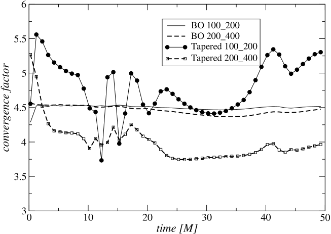
Figure 19: Convergence factors obtained with the numerical solution of $g_{rr}$ for both the BO and tapered boundary approaches. In both cases, a behavior consistent with fourth order accuracy is obtained.

.

Last, we examine the behavior of the errors themselves for the resolutions employed. Figure 20 display the $L_{2}$ norm of the errors $E(g_{rr})\equiv g_{rr}^{n}-g_{rr}^{a}$ with $g_{rr}^{a},g_{rr}^{n}$ the analytical and numerical solution (the latter obtained with $n$ points in the coarse grid). Notice that although both schemes yield a stable evolution, the errors associated with the tapered grid approach are about an order of magnitude smaller than those obtained with the BO scheme.

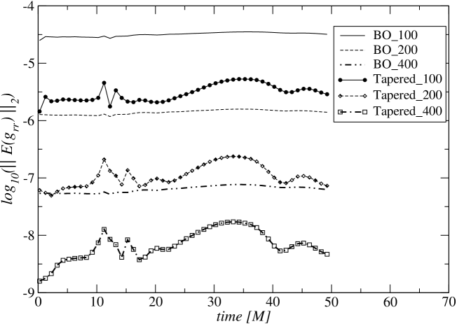
Figure 20: Convergence factors obtained with the numerical solution of $g_{rr}$ for both the BO and tapered boundary approaches. In both cases, a behavior consistent with fourth order accuracy is obtained.

.

III.2 Numerical Results. 3D tests

Semi-linear wave equation

To test these ideas in three dimensions, we use an implementation of the semilinear wave equation. A scalar field $\phi$ obeys the wave equation

$$\Box\phi=Q\phi^{P}$$ (14)

for odd $P$ and where $Q\in\left\{-1,0,1\right\}$ serves to parameterize the nonlinearity. For $Q=0$ the linear case is obtained, whereas for $Q=+1$ the model is focusing (studied in lieblingAMR ) and for $Q=-1$ the model is defocusing. Choosing Cartesian coordinates and defining as the fundamental fields in order to cast the problem in first order differential form:

$$\Pi(x,y,z,t) \equiv \frac{\partial}{\partial t}\phi$$ (15)

$$\Phi_{x}(x,y,z,t) \equiv \frac{\partial}{\partial x}\phi$$ (16)

$$\Phi_{y}(x,y,z,t) \equiv \frac{\partial}{\partial y}\phi$$ (17)

$$\Phi_{z}(x,y,z,t) \equiv \frac{\partial}{\partial z}\phi,$$ (18)

the equation of motion Eq. (14) takes the form of the following system of equations

$$\dot{\phi} = \Pi$$ (19)

$$\dot{\Phi}_{x} = \Pi_{,x}$$ (20)

$$\dot{\Phi}_{y} = \Pi_{,y}$$ (21)

$$\dot{\Phi}_{z} = \Pi_{,z}$$ (22)

$$\dot{\Pi} = \left(\Phi_{x}\right)_{,x}+\left(\Phi_{y}\right)_{,y}+\left(\Phi_{z}\right)_{,z}+Q\phi^{P}.$$ (23)

Solutions of this system are found by incorporating appropriate finite differences within a distributed AMR infrastructure. Using fourth order accurate finite difference approximations of spatial derivatives along with a Runge-Kutta time integrator accurate to third order, convergence to third order is expected as the resolution is increased. This serves also to illustrate that the tapered grid approach allows for decoupling the order of the time-integrator and the derivative operators.

An example of such a convergence test is shown in Fig. 21. A coarse grid with bounds in each direction of $\pm 4$ is established with a (fixed mesh) refined (2:1 refinement) region established with bounds of $\pm 2$. Evolutions were carried out for increasing resolution and the results compared. The lines shown indicate the rescaled differences $C\left(\Pi_{a}-\Pi_{b}\right)$ where $a$ and $b$ indicate the number of points in each dimension, $x$, $y$, and $z$. The rescaling factor $C$ is computed as $C\equiv[1/(145-1)^{3}-1/(181-1)^{3}]/[1/(a-1)^{3}-1/(b-1)^{3}]$ which is how one expects these differences to scale if indeed the code is third order convergent. As the results in the figure show, these differences do decrease as expected. Furthermore, although the size of the differences increase in absolute terms as the pulse propagates across the refinement boundary, convergence and smoothness is not disturbed.

Similar results are obtained for a nonlinear example, as shown in Fig. 22, where a nonlinear case ($Q=1,P=7$) is employed. The initial data describes and incoming pulse which display similar behavior at $t\simeq 2.75$. Our simulations show that even in this highly non-linear regime, the solutions converge to the expected order.

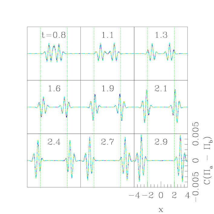
Figure 21: Shown are the differences between runs of various resolutions rescaled according to what would be expected for third order convergence, $C\left(\Pi_{a}-\Pi_{b}\right)$. The initial data consists of an initially static Gaussian pulse centered about the origin for the case where $Q=0$. That the rescaled differences agree, even as the pulse traverses the boundary of the refined region (the green vertical lines), suggests that third order convergence is maintained: red, dotted line ( $\Pi_{145}$ - $\Pi_{181}$), $C=1$, blue, solid line ( $\Pi_{181}$ - $\Pi_{217}$), $C=2.26$, magenta, short dashed line ( $\Pi_{217}$ - $\Pi_{253}$), $C=4.45$, yellow, long dashed line ( $\Pi_{253}$ - $\Pi_{289}$), $C=7.92$, and cyan, dot-short dashed line ( $\Pi_{289}$ - $\Pi_{325}$), $C=13.1$.

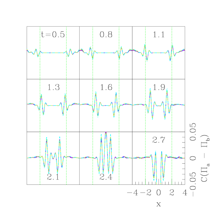
Figure 22: Shown are the various rescaled differences between runs of various resolutions for a nonlinear case ($Q=+1$, $P=7$) of an ingoing wave pulse. The resolutions are the same as those shown in Fig. 21, and similar agreement among them suggests third order convergence. The evolutions demonstrated singular behavior soon after the last frame, placing this evolution confidently within the nonlinear regime of the model.

IV Conclusion and final comments

In the present work we have presented an analysis of different alternatives aiming to yield a stable FMR/AMR implementation. It is observed that the straightforward application of the standard B-O scheme has unstable modes and that natural variations of this scheme share this problem. On the other hand, the tapered boundary approach, in which points that have been affected by the interface boundary treatment are discarded, is clearly stable. In addition to being free of unstable modes, by discarding these points the reflections at the interface between child and parent grids are significantly reduced.

The unstable modes found are represented by eigenvalues of the amplification matrix with norm larger than $1$. An inspection of these reveal that they differ from unity by a small amount (for the toy model considered, and typical grid/CFL values are $\simeq 1.0005$). Therefore, the instabilities associated with these modes will grow slowly for few refinement levels and might not become too evident for evolutions of moderate length. It is thus not surprising that in common applications in numerical relativity where typical CFL factors employed are of order unity, relatively coarse resolutions are employed and the update scheme used is the so-called iterative Crank Nicholson —which is inherently much more dissipative than the Runge-Kutta method considered here— simple test-beds with few levels of refinement do not display unstable modes. For several refinement levels, the instabilities will play a role unless suitably dissipated away. However, we stress again that even if the instabilities might be controlled this way, the errors obtained in all our tests with “standard” approaches are significantly larger than those seen when employing the tapered grid approach.

Other schemes have been recently introduced to reduce the interface reflections for second order methodsbakerAMR . This involves suitably modifying the derivative operators to preserve smoothness in the error of the advection equation at the interfaces. Although the application of these operators give improved results in black hole spacetimes, the results presented did not include sub-cycling and higher derivative schemes have not yet been worked out.

Finally, although we have noticed that the penalty approach does not help in developing a stable AMR strategy, it does play a key role in the stable handling of multiple grid structures that abut multipatch1 . Thus an obvious strategy to implementing AMR techniques within a multiple grid structure is to combine both the penalty technique with the tapered approach. The penalty technique would be used to deal with different grid interfaces while the tapered approach to handle artificial interface boundaries as presented in this work.

Throughout our work we have restricted ourselves to fully first order equations because, in this case, a number of results exist on how to ensure stability of the fully discrete implementation. Such results are not available for fully second order or first order in time/second in space systems, though work in this direction is underwaykreiss2ndorder ; calhinderhusa . Certainly, the tapered approach can still be used in both these types of systems as it only relies on having a stable unigrid implementation and ensuring enough fine grid points in the numerical past domain of dependence at level $n$ to define the solution at level $n+1$.

In summary, the tapered grid approach provides a safe and natural way to build a stable AMR/FMR scheme of arbitrary order. It has a non-trivial overhead cost, but this is offset by the significantly smaller errors and spurious reflections the solutions obtained with it has when compared to existing alternatives. Note: while completing this work a scheme, similar in spirit, for a fourth order implementation has been presented in Csizmadia:2005zq though in this case time and space interpolations are used to fill needed points while the boundary is tapered off.

Appendix A Comparison cost of two ‘stable’ FMR alternatives: 2nd order B-O vs. 4th order tapered

We here compare two stable options for the $u_{,t}=u_{,x}$ problem in their associated computational cost. We concentrate on the relatively inexpensive BO 2nd order scheme and a tapered boundary approach implemented with 4th order accuracy.

The particular issue we concentrate on is whether the additional expense introduced by the 4th order tapered boundary approach renders it too costly to reach a target error when compared with a 2nd order implementation.

To obtain a conservative estimate we assume a base grid with $M+1$ points covering a cubical domain of size $L$ and so we define $h\equiv L/M$. We assume that within this domain, a further refined grid is needed which has $N\simeq M$ points.

Now, suppose one has the option of adopting a 2nd order or a 4th order accurate overall stable scheme. We want to estimate the cost that each one will have associated to it. The computational cost will be determined by the cost of the coarse and fine grid updates. For the coarse grid one needs to take second or fourth order derivatives (which involves two and six operations per point respectively) and the update step (which we take as Runge-Kutta 3rd and 4th order respectively). The cost to update the coarse grids is simply governed by the derivative calculation and the Runge-Kutta update. A simple calculation indicates the cost is $23$ ($38$) floating point operations per point for the second (fourth) order derivative operators plus Runge Kutta 3rd order (4th order). These result from adding the cost associated to computing the different Runge-Kutta steps (ignoring the storage cost), to that of the final update.

The algorithm to update the child grid has four basic steps: A creation of the child grid, B computation of derivatives, C update and D injection from child to parent grid. The cost associated with the child grids for B and C, –per point–, are the same as those in the parent grid. However, since for the 4th order case the child grid must be enlarged, we will here consider that the number of child grid points doubles (hence there will be $N$ and $2N$ points associated to the second and fourth order accurate schemes. This is certainly an exaggeration but serves as a rough upper bound estimate). In addition to the cost associated with the update of the child grid, its creation, step A, via fourth (sixth) order interpolation adds a cost of five (eight) operations per point. Since we adopt a direct injection (i.e. just copying the child grid value on the parent’s at the corresponding point), the floating point operation associated with step D. Hence, the cost of ${\bf B}+{\bf C}$ is $28N$ and $46(2N)$. Combining these numbers one has a total cost of for the second order scheme of $T_{2}=23M+28N$ and $T_{4}=38M+92N$.

Assuming $M\simeq N$ we have for the $3D$ problem $T_{2}\simeq(51N)^{3}$ and $T_{4}\simeq(130N)^{3}$. Thus, $T_{2}/T_{4}\simeq 3^{3}$. Therefore, the 2nd order update scheme could be employed (in this simple and conservative estimate) in a grid that is $3$ times more refined than that of the fourth order scheme with comparable cost. This however does not take into account the errors in the solution obtained with both methods.

To obtain an estimate of this, we can make use of the analysis in ray ; jameson where a comparison of the number of points needed to reach a tolerance error per wavelength is presented. As can be seen in the quoted numbers in Table 1, for a target error $<10^{-2}$ the fourth order accurate scheme is more efficient than the second order one.

We here quote some relevant numbers from ray ,

$\epsilon$	2nd	4th	6th
$10^{-2}$	26	8	6
$10^{-3}$	81	15	9
$10^{-4}$	257	27	13
$10^{-5}$	816	48	19

Table 1: Number of points required per wavelength to achieve a target error $\epsilon$ with second, fourth and sixth order accurate operators.

Hence, the associated extra-cost of a higher order accurate scheme done via the tapered grid approach which discards a non-trivial number of points is offset by the gains in accuracy, and of course, stability of the scheme.

Appendix B Interpolation Operators

B.1 Four point stencils

Points in the child grid lying (as seen from the parent grid) at $x_{i}$ ($i=1..N$) are directly injected from the parent value. The points lying in between coarse points at $x_{i+1/2}$ ($i=1..N-1$) are obtained by the interpolating polynomial,

$$u_{i+1/2} = \frac{1}{160}\left(9(u_{i}+u_{i+1})-(u_{i-1}+u_{i+2})\right)$$ (24)

When excision is employed, the stencil for the second second child grid point must be modified as there are no enough points to one side of it. In this case we employ,

$$u_{3/2} = \frac{1}{128}\left(35u_{1}+140u_{2}-70u_{3}+28u_{4}-5u_{5}\right)$$ (25)

B.2 Six point stencils

As in the previous case, points in the child grid lying (as seen from the parent grid) at $x_{i}$ ($i=1..N$) are directly injected from the parent value. The points lying in between coarse points at $x_{i+1/2}$ ($i=1..N-1$) are obtained by the interpolating polynomial,

$$u_{i+1/2} = \frac{1}{256}\left(150(u_{i}+u_{i+1})-25(u_{i-1}+u_{i+2})+3(u_{i-2}+u_{i+3})\right)$$ (26)

When excision is employed, the stencil for the second and fourth child grids point must be modified as there are no enough points to one side of it. In these cases we employ,

$$u_{3/2} = \frac{1}{256}\left(63u_{1}+315u_{2}-210u_{3}+126u_{4}-45u_{5}+7u_{6}\right)$$ (27)

$$u_{5/2} = \frac{1}{256}\left(-7u_{1}+105u_{2}+210u_{3}-70u_{4}+21u_{5}-3u_{6}\right)$$ (28)

- (1) L. Lehner, Class. Quant. Grav. 18, R25 (2001) [arXiv:gr-qc/0106072].
- (2) M. Miller, arXiv:gr-qc/0502087.
- (3) L. Lehner, O. Reula and M. Tiglio, “Multi-block simulations in general relativity: high order discretizations, numerical stability, and applications,” to appear in Class. Quant. Grav. (2005). arXiv:gr-qc/0507004.
- (4) P. Diener, N. Dorband, E. Schnetter and M. Tiglio. In preparation (2005).
- (5) J. Thornburg, Class. Quant. Grav. 21, 3665 (2004)
- (6) Y. Zlochower, J. G. Baker, M. Campanelli and C. O. Lousto, Phys. Rev. D 72, 024021 (2005).
- (7) G. Calabrese and D. Neilsen, Phys. Rev. D 71, 124027 (2005)
- (8) M. W. Choptuik, E. W. Hirschmann, S. L. Liebling and F. Pretorius, Phys. Rev. Lett. 93, 131101 (2004). F. Pretorius and L. Lehner, J. Comput. Phys. 198, 10 (2004) S. L. Liebling, Phys. Rev. D 71, 044019 (2005). F. Pretorius, Class. Quant. Grav. 22, 425 (2005). E. Evans, S. Iyer, E. Schnetter, W. M. Suen, J. Tao, R. Wolfmeyer and H. M. Zhang, Phys. Rev. D 71, 081301 (2005) F. Pretorius and M. W. Choptuik, arXiv:gr-qc/0508110. (2005).
- (9) B. Zink, N. Stergioulas, I. Hawke, C. D. Ott, E. Schnetter and E. Muller, arXiv:gr-qc/0501080 (2005). U. Sperhake, B. Kelly, P. Laguna, K. L. Smith and E. Schnetter, Phys. Rev. D 71, 124042 (2005). B. Bruegmann, W. Tichy and N. Jansen, Phys. Rev. Lett. 92, 211101 (2004). E. Schnetter, S. H. Hawley and I. Hawke, Class. Quant. Grav. 21, 1465 (2003).
- (10) G. Calabrese, L. Lehner, D. Neilsen, J. Pullin, O. Reula, O. Sarbach and M. Tiglio, Class. Quant. Grav. 20, L245 (2003)
- (11) G. Calabrese, L. Lehner, O. Reula, O. Sarbach and M. Tiglio, Class. Quant. Grav. 21, 5735 (2004)
- (12) L. Lehner, D. Neilsen, O. Reula and M. Tiglio, Class. Quant. Grav. 21, 5819 (2004)
- (13) D. Levy and E. Tadmor, SIAM Journal on Num. Anal 40, 40, (1998).
- (14) M. Berger, Mathematics of Computation 45, N172, 301 (1985).
- (15) R.A. Trompert and J. G. Verwer, Mathematics of Computation 6, N202, 591 (1993).
- (16) J. Oliger and X. Zhu, Applied Numerical Mathematics, 20, 407 (1996).
- (17) M.J. Berger, and J. Oliger. ”Adaptive Mesh Refinement for hyperbolic partial differential equations,” J. Comp. Phys. 53, 484 (1984).
- (18) M. Carpenter, D. Gottlieb and S. Abarbanel, J. Comput. Phys. 111 (1994)
- (19) M. Carpenter, J. Nordstrom, and D. Gottlieb, J. Comput. Phys. 148, 2, 341 (1999).
- (20) O. Sarbach and M. Tiglio, Phys. Rev. D 70, 104018 (2004).
- (21) L. E. Kidder, M. A. Scheel, S. A. Teukolsky, E. D. Carlson and G. B. Cook, Phys. Rev. D 62, 084032 (2000)
- (22) G. Calabrese, L. Lehner and M. Tiglio, Phys. Rev. D 65, 104031 (2002)
- (23) S. L. Liebling, Phys. Rev. D 71, 044019 (2005).
- (24) J. G. Baker and J. R. Meter, arXiv:gr-qc/0505100.
- (25) B. Szilagyi, H. O. Kreiss and J. Winicour, Phys. Rev. D 71, 104035 (2005).
- (26) G. Calabrese, I. Hinder and S. Husa, arXiv:gr-qc/0503056.
- (27) P. Csizmadia, arXiv:hep-th/0505036.
- (28) J. Ray, C.A. Kennedy, S. Lefanty and H.N. Najm. ”High order spatial discretizations and extended stability methods for reacting flows on structured adaptively refined meshes”. Proceedings of the Third Joint meeting of the U.S. Section of the Combustions Institute. (2003).
- (29) L. Jameson. “AMR vs high-order schemes, wavelets as a guide”. Technical Report UCRL-ID 141537, Lawrence Livermore National Laboratory, Livermore, California 2000.
- (30) M. W. Choptuik, Phys. Rev. Lett. 70, 9 (1993).
- (31) P. Olsson, Math. Comp. 64, 1035 (1995); 64 S23 (1995); 64, 1473 (1995).
- (32) B. Gustafsson, H. Kreiss, and J. Oliger “Time dependent problems and difference methods”, John Wiley and Sons, 1995.
- (33) H. Kreiss and J. Oliger, GARP Publication Series 10, World Meteorological Organization, Geneva (1973).