Self-stabilization of extra dimensions

Abstract

We show that the problem of stabilization of extra dimensions in Kaluza-Klein type cosmology may be solved in a theory of gravity involving high-order curvature invariants. The method suggested (employing a 3 slow-change approximation) can work with rather a general form of the gravitational action. As examples, we consider pure gravity with Lagrangians quadratic and cubic in the scalar curvature and some more complex ones in a simple Kaluza-Klein framework. After a transition to the 4D Einstein conformal frame, this results in effective scalar field theories with certain effective potentials, which in many cases possess positive minima providing stable small-size extra dimensions. Estimates made in the original (Jordan) conformal frame show that the problem of a small value of the cosmological constant in the present Universe is softened in this framework but is not solved completely.

Short title: Self-stabilization of extra dimensions

I Introduction

Modern cosmology is able to explain many properties of our Universe due to a substantial progress in experimental methods and technology and development of new theoretical models. Nevertheless, there is quite a number of long-standing and challenging unsolved problems. We are going to discuss some of them. The first one, known for two decades, concerns the origin and form of the inflaton potential Lindebook able to provide a sufficient primordial inflation satisfying the observational constraints. Despite numerous attempts, see, e.g., Hybrid ; Massive , the problem is yet to be solved. Another problem is related to the recently observed accelerated expansion of the Universe whose origin is usually ascribed to some unknown and invisible dark energy, which is likely to be identified with an extremely small but nonzero vacuum energy density, or cosmological constant. Certain problems of theoretical origin are common to all modern theories, employing the idea of extra dimensions, among which well-known are M-theory, supergravities, diverse Kaluza-Klein and brane-world scenarios. A requirement which inevitably accompanies such investigations is that the extra dimensions should be invisible since our space-time looks 4-dimensional at least at scales over $10^{-17}$ cm. In models where the extra dimensions are assumed to be compact, this is a severe restriction on their size. Moreover, to account for the observed constancy or nearly constancy of the fundamental physical constants (the gravitational constant $G$, the fine structure constant $\alpha$ and others constants ), this size should be constant and stable, and therefore a mechanism of stabilization of the extra dimensions is required in any scenario that involves them.

The most popular way of reaching such a stabilization is to invoke a scalar field of non-geometric origin with an appropriate potential. This new entity seems somewhat artificial because scalar fields already exist in this framework: the metric tensor components corresponding to the extra dimensions behave as scalar and vector fields in our 4D space. It is, however, difficult to obtain a suitable form of the potential for such fields Kolb ; Mazumdar . To improve the situation, additional non-gravitational fields are invoked thus returning us to the starting point.

On the other hand, the gravitational action, in general, includes terms containing nonlinear functions of the Ricci scalar as well as other curvature invariants. Such nonlinear terms inevitably appear if one takes into account quantum phenomena gmm ; bird ; Don . In fact, the first model of inflation was based on this idea Star80 . Gravity represents a wide choice of different forms of action since even renormalization of non-gravitational quantum fields against a curved background yields various curvature terms with indefinite coefficients, to say nothing of presently unknown classical “traces” of quantum gravity and Casimir-like contributions from a nontrivial space-time topology (if any). This wealth of possibilities has a negative imprint. Indeed, only one form of the gravitational action among many is realized in our Universe, and it is a challenging problem to choose the correct one.

In this paper, we study curvature-nonlinear gravity in a space-time manifold with an arbitrary number of extra dimensions. Our aim is threefold. First, we intend to demonstrate that even the simplest version of nonlinear multidimensional gravity (with the Lagrangian $F(R)$, $R$ being the Ricci scalar) leads to a scalar field with potential and kinetic terms having promising shapes. Second, we are going to point out some particular examples of minima of the effective potential $V$ with positive $V=V_{\min}$, which are, in principle, able to describe the present accelerated expansion of the Universe (certainly in a very rough approximation). Third, we try to find out whether or not, or to which extent, the well-known cosmological constant problem can be solved in the present class of theories.

In our study we use the slow-change approximation, assuming smallness of all derivatives, in a sense discussed below, and smallness of energy densities compared to the Planck scale. Such assumptions are rather widespread in studies of inflationary scenarios. This method allows dealing with rather general forms of the gravitational action and extended parameter ranges. With its help, new minima of the potential which can provide stability and smallness of the extra dimensions are found.

The paper is organized as follows. In Sec. II we consider $F(R)$ theories of gravity in multidimensional space-times where the extra dimensions comprise a constant-curvature space with a scale factor $b(x)$, depending on the external (observed) coordinates. Integrating out the extra dimensions in the action and applying the slow-change approximation, we obtain an effective scalar-tensor theory in 4 dimensions with a single scalar field $b(x)$ and specific forms of its potential and kinetic terms. It should be noted that the complexity of the kinetic term can also affect the system dynamics and qualitatively change its properties Kessence ; Ru04 .

We also show that our approximation agrees with the conventional approach that reduces $F(R)$ gravity to $D$-dimensional Einstein gravity coupled to a scalar field with a potential related to $F(R)$.

Sec. III is devoted to numerical estimates concerning possible stationary states of the extra dimensions. We briefly discuss the role of conformal frames, distinguishing the fundamental frame in which the theory is originally formulated (saying what happens as a matter of fact) and the frame used to interpret the observations (showing what we can see). The choice of the latter depends on the properties of references employed in our measurements pictures . We here restrict ourselves to the simplest and maybe the most natural assumption, that the observational frame coincides with the fundamental (Jordan) one. Under this assumption, it turns out that the smallness of the present cosmological constant remains a problem though less severe than in conventional cosmology.

In Sec. IV we use our method for seeking stable states of the extra dimensions in quadratic multidimensional gravity, with $F(R)=R+cR^{2}-2\Lambda$ where $c$ and $\Lambda$ are constants. This theory has been previously discussed in Ref. Zhuk , where local minima of the potential $V$ with $V_{\min}<0$ were found at values of $R$ corresponding to $dF/dR>0$. In the cosmological context, such minima can only lead to models with the anti-de Sitter space AdS₄. We confirm this result but also find new minima of the potential in the unusual range where $dF/dR<0$; for some of them, $V_{\min}>0$, which leads to de Sitter cosmology.

Sec. V discusses other choices of the initial Lagrangian. Thus, with $F(R)$ taken in the form of a cubic polynomial, we find minima of the effective potential with $V_{\min}>0$ in the region where $dV/dR>0$. Then we demonstrate that our method can be successfully applied to a much wider class of multidimensional theories of gravity, e.g., those containing the Ricci tensor squared and the Kretschmann scalar. Sec. VI contains some concluding remarks.

II $F(R)$ theory in $D$ dimensions

II.1 Basic equations

We consider a $(D=d_{0}+d_{1})$-dimensional manifold with the metric

$$ds^{2}=g_{\mu\nu}dx^{\mu}dx^{\nu}+{\,\rm e}^{2\beta(x)}b_{ab}dx^{a}dx^{b}$$ (1)

where the extra-dimensional metric components $b_{ab}$ are independent of $x^{\mu}$, the observable space-time coordinates. The relevant case is certainly $d_{0}=4$ but, in Eqs. (II.1)–(5), we keep $d_{0}$ arbitrary for generality.

The $D$-dimensional Riemann tensor has the nonzero components

$$R^{\mu\nu}{}_{\rho\sigma} \!= \!{\overline{R}}^{\mu\nu}{}_{\rho\sigma},$$

$${}R^{\mu a}{}_{\nu a} \!= \!\delta^{a}_{b}\,B_{\nu}^{\mu},\hskip 28.45274ptB_{\nu}^{\mu}:={\,\rm e}^{-\beta}\nabla_{\nu}({\,\rm e}^{\beta}\beta^{\mu}),$$

$${}R^{ab}{}_{cd} \!= \!{\,\rm e}^{-2\beta}{\overline{R}}^{ab}{}_{cd}+\delta^{ab}{}_{cd}\beta_{\mu}\beta^{\mu},$$ (2)

where capital Latin indices cover all $D$ coordinates, the bar marks quantities obtained from $g_{\mu\nu}$ and $b_{ab}$ taken separately, $\beta_{\mu}\equiv\partial_{\mu}\beta$ and $\delta^{ab}{}_{cd}\equiv\delta_{c}^{a}\delta_{d}^{b}-\delta_{d}^{a}\delta_{c}^{b}$. The nonzero components of the Ricci tensor and the scalar curvature are

$$R_{\mu}^{\nu} \!= \!{\overline{R}}_{\mu}^{\nu}+d_{1}\,B_{\mu}^{\nu},$$

$${}R_{a}^{b} \!= \!{\,\rm e}^{-2\beta}{\overline{R}}_{a}^{b}+\delta_{a}^{b}[\mathop{\raisebox{-0.5pt}{$\Box$}}\nolimits\beta+d_{1}(\partial{\beta})^{2}],$$

$${}R \!= \!{\overline{R}}[g]+{\,\rm e}^{-2\beta}{\overline{R}}[b]+2d_{1}\mathop{\raisebox{-0.5pt}{$\Box$}}\nolimits\beta+d_{1}(d_{1}+1)(\partial{\beta})^{2},$$

where $(\partial{\beta})^{2}\equiv\beta_{\mu}\beta^{\mu}$, $\mathop{\raisebox{-0.5pt}{$\Box$}}\nolimits=g^{\mu\nu}\nabla_{\mu}\nabla_{\nu}$ is the $d_{0}$-dimensional d’Alembert operator while ${\overline{R}}[g]$ and ${\overline{R}}[b]$ are the Ricci scalars corresponding to $g_{\mu\nu}$ and $b_{ab}$, respectively.

Suppose now that $b_{ab}$ describes a $d_{1}$-dimensional space of nonzero constant curvature, i.e., a sphere ($k=1$) or a compact $d_{1}$-dimensional hyperbolic space Lob ($k=-1$) with a fixed curvature radius $r_{0}$ normalized to the $D$-dimensional analogue $m_{\scriptscriptstyle D}$ of the Planck mass, i.e., $r_{0}=1/m_{\scriptscriptstyle D}$ (we use the natural units, with the speed of light $c$ and Planck’s constant $\hbar$ equal to unity). We have

$${\overline{R}}^{ab}{}_{cd} \!= \!k\,m_{\scriptscriptstyle D}^{2}\,\delta^{ab}{}_{cd},\hskip 28.45274pt{\overline{R}}_{a}^{b}=k\,m_{\scriptscriptstyle D}^{2}\,(d_{1}-1)\delta_{a}^{b},$$

$${}{\overline{R}}[b] \!= \!k\,m_{\scriptscriptstyle D}^{2}\,d_{1}(d_{1}-1)=R_{b}.$$ (4)

The scale factor $b(x)\equiv{\,\rm e}^{\beta}$ in (1) is thus kept dimensionless; $R_{b}$ has the meaning of a characteristic curvature scale of the extra dimensions.

Consider, in the above geometry, a sufficiently general curvature-nonlinear theory of gravity with the action

$$S={{\displaystyle\frac{1}{2}}}m_{\scriptscriptstyle D}^{D-2}\int\sqrt{{}^{D}g}\,d^{D}x\,[F(R)+L_{m}],$$ (5)

where $F(R)$ is an arbitrary smooth function, $L_{m}$ is a matter Lagrangian and ${{}^{D}}g=|\det(g_{MN})|$. The extra coordinates are easily integrated out, and the action is reduced to $d_{0}=4$ dimensions:

$$S={{\displaystyle\frac{1}{2}}}{\cal V}[d_{1}]\,m_{\scriptscriptstyle D}^{2}\int\sqrt{{}^{4}g}\,d^{4}x\,{\,\rm e}^{d_{1}\beta}\,[F(R)+L_{m}],$$ (6)

where ${}^{4}g=|\det(g_{\mu\nu})|$ and ${\cal V}[d_{1}]$ is the volume of a compact $d_{1}$-dimensional space of unit curvature.

II.2 Slow-change approximation. The Einstein frame

Eq. (6) describes a 4D theory which is nonlinear in curvature and, moreover, contains a non-minimal coupling between the effective scalar field $\beta$ and the curvature. Let us simplify it in the following manner:

(a) Express everything in terms of 4-dimensional variables and $\beta(x)$; note that now

$${}R=R_{4}+\phi+f_{1},$$

$${}R_{4}={\overline{R}}[g],\qquad f_{1}=2d_{1}\mathop{\raisebox{-0.5pt}{$\Box$}}\nolimits\beta+d_{1}(d_{1}+1)(\partial{\beta})^{2},$$ (7)

and we have introduced the effective scalar field

$$\phi(x)=R_{b}{\,\rm e}^{-2\beta(x)}=kd_{1}(d_{1}-1)m_{\scriptscriptstyle D}^{2}\,{\,\rm e}^{-2\beta(x)}.$$ (8)

Recall that we have $k=\pm 1$ for positive and negative curvature in $d_{1}$ extra dimensions, respectively, so that $\phi$ has different signs in these cases by definition.

(b) Suppose that all quantities are slowly varying, i.e., consider each derivative $\partial_{\mu}$ (including those in the definition of ${\overline{R}}$) as an expression containing a small parameter $\varepsilon$; neglect all quantities of orders higher than $O(\varepsilon^{2})$ (see Don ).

(c) Perform a conformal mapping leading to the Einstein conformal frame, where the 4-curvature appears to be minimally coupled to the scalar $\phi$.

In the decomposition (II.2), both terms $f_{1}$ and $R_{4}$ are regarded small in our approach, which actually means that all quantities, including the 4D curvature, are small compared to the $D$-dimensional Planck scale. So the only term which is not small is $\phi$, and we can use a Taylor decomposition of the function $F(R)=F(\phi+R_{4}+f_{1})$:

$$F(R)=F(\phi+R_{4}+f_{1})\simeq F(\phi)+F^{\prime}(\phi)\cdot(R_{4}+f_{1})+...,$$ (9)

with $F^{\prime}(\phi)\equiv dF/d\phi$. Substituting it into Eq. (6), we obtain up to $O(\varepsilon^{2})$

$${}S={{\displaystyle\frac{1}{2}}}{{\cal V}[d_{1}]}\,m_{\scriptscriptstyle D}^{2}\int\sqrt{{}^{4}g}\,d^{4}x\,{\,\rm e}^{d_{1}\beta}[F^{\prime}(\phi)R_{4}\hskip 28.45274pt$$

$${}\hskip 72.26999pt+F(\phi)+F^{\prime}(\phi)f_{1}+L_{m}],$$ (10)

where $\beta$ is related to $\phi$ according to (8). The expression (II.2) is typical of a scalar-tensor theory (STT) of gravity in a Jordan frame.

To find stationary points, it is helpful to pass on to the Einstein frame. After the conformal mapping

$$g_{\mu\nu}\ \mapsto{\widetilde{g}}_{\mu\nu}=|f(\phi)|g_{\mu\nu},\hskip 28.45274ptf(\phi)={\,\rm e}^{d_{1}\beta}F^{\prime}(\phi),$$ (11)

with the corresponding transformation of the scalar curvature

$$R_{4}=|f|\biggl{(}{\widetilde{R}}_{4}+\frac{3}{f}{\widetilde{\mathop{\raisebox{-0.5pt}{$\Box$}}}\nolimits}f-\frac{3}{2f^{2}}(\widetilde{\partial}f)^{2}\biggr{)}$$ (12)

(the tilde marks quantities obtained from or with ${\widetilde{g}}_{\mu\nu}$), the action (II.2) acquires the form

$${}S={{\displaystyle\frac{1}{2}}}{{\cal V}[d_{1}]}\,m_{\scriptscriptstyle D}^{2}\int\sqrt{{\widetilde{g}}}\,d^{4}x\biggl{\{}[\mathop{\rm sign}\nolimits F^{\prime}(\phi)]\ [{\widetilde{R}}_{4}+K]$$

$${}\hskip 28.45274pt\hskip 28.45274pt-V(\phi)+\frac{{\,\rm e}^{-d_{1}\beta}}{F^{\prime}(\phi)^{2}}L_{m}\biggr{\}}$$ (13)

with the kinetic ($K$) and potential ($V$) terms

$$K \!= \!\frac{3}{2}\frac{(\partial f)^{2}}{f^{2}}-2d_{1}\frac{f^{,\mu}\beta_{\mu}}{f}+(\partial\beta)^{2},$$

$${}V(\phi) \!= \!-{\,\rm e}^{-d_{1}\beta}\,F(\phi)/F^{\prime}(\phi)^{2}.$$ (14)

It remains to express everything in terms of a single scalar variable, say, $\phi$. We can write the action (II.2) in the form

$$S \!= \!\frac{{\cal V}[d_{1}]}{2}m_{\scriptscriptstyle D}^{2}\int\sqrt{{\widetilde{g}}}\,(\mathop{\rm sign}\nolimits F^{\prime})L,$$

$${}L \!= \!{\widetilde{R}}_{4}+{{\displaystyle\frac{1}{2}}}K_{\rm Ein}(\phi)(\partial\phi)^{2}-V_{\rm Ein}(\phi)+{\widetilde{L}}_{m},$$ (15)

$${}\ \ {\widetilde{L}}_{m}=(\mathop{\rm sign}\nolimits F^{\prime})\frac{{\,\rm e}^{-d_{1}\beta}}{F^{\prime}(\phi)^{2}}L_{m};$$

$$K_{\rm Ein}(\phi) \!= \!\frac{1}{2\phi^{2}}\left[6\phi^{2}\biggl{(}\frac{F^{\prime\prime}}{F^{\prime}}\biggr{)}^{2}\!-2d_{1}\phi\frac{F^{\prime\prime}}{F^{\prime}}+{{\displaystyle\frac{1}{2}}}d_{1}(d_{1}{+}2)\right],$$

$$V_{\rm Ein}(\phi) \!= \!-(\mathop{\rm sign}\nolimits F^{\prime})\left[\frac{|\phi|m_{\scriptscriptstyle D}^{-2}}{d_{1}(d_{1}-1)}\right]^{d_{1}/2}\frac{F(\phi)}{F^{\prime}(\phi)^{2}}$$ (17)

In (12)–(15), the indices are raised and lowered with ${\widetilde{g}}_{\mu\nu}$; everywhere $F=F(\phi)$ and $F^{\prime}=dF/d\phi$.

Eqs. (15)–(17) are valid for both positive ($\phi>0$) and negative ($\phi<0$) curvature of the extra dimensions. Minima of the potential $V_{\rm Ein}$, defined in the Einstein frame, determine stationary points of the scalar field, and they remain to be stationary points after a transition to any other conformal frame, including the original Jordan frame. It is the Einstein frame that determines the scalar field behavior since its dynamics near an extremum is governed directly by the potential $V(\phi)$ and only implicitly by the metric.

If $\phi$ resides at a minimum of the potential $V_{\rm Ein}$, this potential turns into an effective cosmological constant. Being applied to the present cosmological epoch, it can determine the observable dark energy density that drives the accelerated expansion of the Universe. Alternatively, in principle, it may drive inflation in the early Universe.

We have achieved one of our goals: the potential (17) valid for any function $F(R)$ looks quite complex to have some nontrivial extrema. In addition, we have obtained rather a complex form of the kinetic term (II.2). Its properties are known to be as important for the field dynamics as the shape of the potential. For example, as shown in Ref. Ru04 , zeros and singular points of the kinetic term may be responsible for stable states of a scalar field.

In our expressions, both the effective potential (17) and the kinetic term (II.2) are singular at the values of $\phi$ where $f(\phi)\sim F^{\prime}(R)$ [the factor before $R_{4}$ in the Jordan-frame action (II.2)] is zero. Unlike many papers restricted to $F^{\prime}(R)>0$, we also include models with $F^{\prime}(R)<0$. As will be seen below, this opens new promising possibilities such as new minima of the effective potential at which the extra dimensions may be stabilized. Moreover, models with conformal continuations vac4 ; hog1 , which unify regions with $F^{\prime}>0$ and $F^{\prime}<0$, are possible; these regions correspond to different Einstein-frame manifolds but turn out to be smoothly connected in the Jordan frame. Though, such models are likely to be unstable, as follows from the experience of dealing with different solutions of scalar-tensor theories instab . Our main interest here is in other values of $\phi$, namely, those at which it may be stabilized.

In (15)–(17) we have actually changed the sign of the Lagrangian in the case $F^{\prime}<0$; to preserve the attractive nature of gravity for ordinary matter, the matter Lagrangian density should appear with an unusual sign from the beginning. As a result, the sign of the whole action of gravity and matter will be unusual, without any effect on the matter equations of motion, and the conventional form of the effective Einstein equations at a stationary value of $\phi$ will also be preserved. Only the action of the $\phi$ field itself can be unusual, according to Eqs. (II.2), (17). It should be noted that the common sign of the total action does not affect quantum transitions as well. Indeed, the transition amplitude is expressed in the path integral technique as $\int\exp{(iS[q])}Dq$ where $q(t)$ is some dynamical variable. The transition probability $\int\int\exp{(iS[q_{1}]-iS[q_{2}])}Dq_{1}Dq_{2}$ is invariant under the substitution $i\to-i$ (with interchanging the integration variables $q_{1}$ and $q_{2}$).

II.3 Comparison with the conventional approach

There is a well-known conformal mapping f(R) bringing the theory (5) to the form of general relativity with a minimally coupled scalar field $\chi$ that replaces the additional degrees of freedom connected with $R$:

$$g_{AB} \!= \!{\,\rm e}^{-2\omega(\chi)}h_{AB},$$

$${}\chi \!= \!\pm\sqrt{\frac{D-1}{D-2}}\ln|F_{R}|,\quad\ {\,\rm e}^{\omega}(\chi)=|F_{R}|^{1/(D-2)},$$ (18)

with $F_{R}\equiv dF/dR$. This results in a $D$-dimensional Einstein frame, with the action

$${}S=S_{DE}[h]={{\displaystyle\frac{1}{2}}}m_{\scriptscriptstyle D}^{D-2}\int\sqrt{{}^{D}h}\,d^{D}x$$

$${}\times\biggl{\{}(\mathop{\rm sign}\nolimits F_{R})\bigl{[}R[h]+(\partial\chi)^{2}_{h}]-2V(\chi)+L_{m}{\,\rm e}^{-D\omega}\biggr{\}},$$

$${}\hskip 28.45274pt2V(\chi)={\,\rm e}^{-D\omega}(RF_{R}-F),$$ (19)

where $R[h]$ is the Ricci scalar obtained from $h_{AB}$, ${}^{D}h=|\det(h_{AB})|$ and $(\partial\chi)^{2}_{h}=h^{AB}\chi_{,A}\chi_{,B}$; the initial Ricci scalar $R$ is considered as a function of $\chi$.

(An even more general transformation is known maeda , bringing a $D$-dimensional theory of gravity whose Lagrangian contains an arbitrary function of two variables, $f(R,\phi)$, to an Einstein frame with two minimally coupled scalar fields, $\phi$ and the one similar to $\chi$. Maeda’s method maeda generalizes the corresponding mappings known for both scalar-tensor wagon and $f(R)$ f(R) theories of gravity.)

The theory (II.3) may be further reduced to 4 dimensions and brought with one more conformal mapping, now depending on $\beta(x)$ and similar to (11), to a 4-dimensional Einstein frame. Reduction in terms of the metric $h_{AB}$ gives

$${}S=S_{4J}[h]={{\displaystyle\frac{1}{2}}}m_{\scriptscriptstyle D}^{D-2}{\cal V}[d_{1}]\int d^{4}x\,\sqrt{{}^{4}h}\,{\,\rm e}^{d_{1}\alpha}$$

$${}\times\biggl{\{}(\mathop{\rm sign}\nolimits F_{R})\biggl{[}R_{4}[h]+(\partial\chi)^{2}_{h}-d_{1}(d_{1}-1)(\partial\alpha)^{2}_{h}$$

$${}\hskip 28.45274pt\hskip 28.45274pt-{\,\rm e}^{-2\alpha}R_{b}\biggr{]}-2V(\chi)+L_{m}{\,\rm e}^{-D\omega}\biggr{\}},$$

$${}\alpha:=\beta+\omega,$$ (20)

where ${}^{4}h=|\det(h_{\mu\nu})|$. After a further transformation,

$$h_{\mu\nu}={\,\rm e}^{-d_{1}\alpha}\gamma_{\mu\nu},$$ (21)

we arrive at a theory defined in the 4D Einstein frame with the metric $\gamma_{\mu\nu}$. The action is

$${}S=S_{4E}[\gamma]={{\displaystyle\frac{1}{2}}}m_{\scriptscriptstyle D}^{D-2}{\cal V}[d_{1}]\int\sqrt{\gamma}\,d^{4}x\,$$

$${}\times\biggl{\{}(\mathop{\rm sign}\nolimits F_{R})\biggl{[}R[\gamma]+(\partial\chi)^{2}_{\gamma}+{{\textstyle\frac{1}{2}}}d_{1}(d_{1}+2)(\partial\alpha)^{2}_{\gamma}$$

$${}-{\,\rm e}^{-(d_{1}+2)\alpha}R_{b}\biggr{]}-2V(\chi){\,\rm e}^{-d_{1}\alpha}+L_{m}{\,\rm e}^{-D\omega-d_{1}\alpha}\biggr{\}},$$ (22)

with $\gamma=|\det(g_{\mu\nu})|$ and $(\partial\chi)^{2}_{\gamma}=\gamma^{\mu\nu}\chi_{,\mu}\chi_{,\nu}$.

Evidently, under the conditions of our slow-change approximation, the action (II.3) should lead to the same results as (II.2). Let us confirm that it is indeed the case, assuming in (II.3) that all derivatives $\partial_{\mu}$ involve a small parameter. We have, as before, (9) and similarly

$$F_{R}=F^{\prime}(\phi)+F^{\prime\prime}(\phi)(R_{4}+F_{1})+...,$$ (23)

where $R_{4}=R_{4}[g]$. Then, comparing the transitions $g_{AB}\to g_{\mu\nu}\to{\widetilde{g}}_{\mu\nu}$ in (11) and $g_{AB}\to h_{AB}\to h_{\mu\nu}\to\gamma_{\mu\nu}$, we see that the two Einstein-frame metrics ${\widetilde{g}}$ and $\gamma$ are related by

$${\widetilde{g}}_{\mu\nu}=\frac{F^{\prime}(\phi)}{F_{R}}\gamma_{\mu\nu}=\biggl{[}1+\frac{F^{\prime\prime}(\phi)}{F^{\prime}(\phi)}(R_{4}+f_{1})+...\biggr{]}\gamma_{\mu\nu}$$ (24)

and coincide in the leading order of magnitude. The leading terms of the actions (15) and (II.3), represented by their potential and matter terms, should then also coincide, and it is easy to confirm that it is really the case (the term $RF_{R}$ in (II.3) transforms to $\phi F^{\prime}(\phi)$ and is cancelled by the term with ${\mathbb{R}}_{b}$, leading to the expression (17) for the $\phi$ field potential).

It is also seen that both fields $\chi$ and $\alpha$ are reduced, in the same approximation, to the $\phi$ field defined in Eq. (8):

$$\alpha_{,\mu}\approx\beta_{,\mu}+\frac{1}{D-2}\frac{F^{\prime\prime}}{F^{\prime}}\phi_{,\mu},\quad\chi_{,\mu}\approx\sqrt{\frac{D-1}{D-2}}\frac{F^{\prime\prime}}{F}\phi_{,\mu},$$ (25)

and $\beta_{,\mu}=-\phi_{,\mu}/(2\phi)$. As a result, the whole kinetic term takes precisely the form (II.2). So the action (15) is completely restored.

One can note, however, that our approximation, being applied from the very beginning, not only makes things simpler but is more universal: it can deal with actions more general than (5) (see Sec. V).

III Effective constants: some estimates

III.1 Conformal frames and requirements to the model

To relate the theory to Nature, it is necessary to specify which conformal frame is to be confronted to observations.

In our problem setting, the Jordan frame described above appears to be fundamental since the initial theory is formulated in it, and the quantum effects that give rise to the nonlinearity of gravity are also supposed to take place there.

It is, however, quite unnecessary to believe that this Jordan frame corresponds to the observed picture, in which the properties of our measurement instruments and the standards of the relevant physical units do not change in space and time pictures . The latter is thus the frame in which the basic atomic units (depending, above all, on fermion masses) are constant, if certainly they are all constant simultaneously. How sensitive is the matter Lagrangian to conformal mappings is even well seen from the coefficient before $L_{m}$ in Eq. (15), to say nothing of a nontrivial metric dependence of matter fields entering into $L_{m}$.

Since we here do not specify how fermions are included into the theory, it is only possible to assume which is the observational frame. We will here dwell upon, probably, the most natural choice and make some estimates in the Jordan frame thus assuming that the basic and observational frames coincide.

As regards the Einstein frame in which the action takes the form (II.2), we simply use it as a technical trick to determine stationary states.

In any observational frame, in the expected stationary state, the gravitational action has the approximate Einstein-Hilbert form

$$S_{\rm GR}={{\displaystyle\frac{1}{2}}}m_{4}^{2}\int\sqrt{{}^{4}g}\,d^{4}x\,(R_{4}^{*}-2\Lambda_{\rm eff}),$$ (26)

where $m_{4}=(8\pi G_{N})^{-1/2}$ is the 4D Planck mass, $G_{N}$ is the effective Newtonian constant and $R^{*}_{4}$ is the observable 4D curvature (for our choice, $R_{4}^{*}=R_{4}$). To be consistent with our approach and with observational constraints, this stationary state should satisfy the following requirements:

(i)

A classical space-time description should be admissible, i.e., the true size of the extra dimensions should exceed the true $D$-dimensional Planck length $1/m_{\scriptscriptstyle D}$, the fundamental length scale of the theory:

$$m_{\scriptscriptstyle D}b_{0}={\,\rm e}^{\beta_{0}}\gg 1,\quad{\rm or}\quad\phi/m_{\scriptscriptstyle D}^{2}\ll d_{1}(d_{1}-1).$$ (27)

(ii)

The slow-change approximation should work, which, for $\phi={\rm const}$, reduces to the requirement $R_{4}\ll m_{D}^{2}$.

(iii)

The observed size $b^{*}$ of the extra dimensions can be much larger than the Planck length $l_{4}=1/m_{4}\approx 8\mbox{$\cdot 10^{-33}$}$ cm, but not larger than about $10^{-17}$ cm, which corresponds to the TeV energy scale.

(iv)

The predicted effective cosmological constant $\Lambda_{\rm eff}$ should be very small to conform to the observations:

$$\Lambda_{\rm eff}/m_{4}^{2}\sim 10^{-120}$$ (28)

(the exponent is $-120$ instead of more conventional $-122$ because the definition of $m_{4}$ involves $8\pi$).

Obtaining such a small value as (28) is one of the well-known problems of theoretical cosmology since it is hard to explain without fine tuning why $\Lambda m_{4}^{2}$, generally associated with vacuum energy density, is so many orders of magnitude smaller than the characteristic energy densities inherent to the known physical interactions (e.g., the Planck density $m_{4}^{4}$ for gravity).

III.2 Estimates in the Jordan frame

Thus we assume that observations are performed in the Jordan frame. The corresponding action (II.2) is approximated by (26) with the effective constants

$$\frac{1}{8\pi G_{N}}=m_{4}^{2}={\cal V}[d_{1}]\,m_{\scriptscriptstyle D}^{D-2}\,b_{0}^{d_{1}}F^{\prime}_{0},\quad\ \Lambda_{\rm eff}=-\frac{F(\phi_{0})}{2F^{\prime}_{0}},$$ (29)

where $b_{0}={\,\rm e}^{\beta(\phi_{0})}/m_{\scriptscriptstyle D}=b_{*}$ is the observable size of the extra dimensions and $F^{\prime}_{0}=F^{\prime}(\phi_{0})$.

Eq. (29) leads to the following relation between the dimensionless quantities $b_{0}m_{\scriptscriptstyle D}$ and $b_{0}m_{4}$:

$$b_{0}^{2}m_{4}^{2}={\cal V}[d_{1}]\,F^{\prime}_{0}\,(b_{0}m_{\scriptscriptstyle D})^{d_{1}+2}.$$ (30)

The factor ${\cal V}[d_{1}]$ is of order unity; the same may be expected from the dimensionless quantity $F^{\prime}_{0}$. By item (iii) above, $b_{0}^{2}m_{4}^{2}\ \,\raisebox{3.0pt}{${\mathop{<}\limits_{\textstyle\sim}}$}\,\ 10^{30}$, and Eq. (30) gives

$${}b_{0}m_{\scriptscriptstyle D}\lesssim 10^{30/(d_{1}+2)},$$

$${}m_{4}/m_{\scriptscriptstyle D}\sim(b_{0}m_{\scriptscriptstyle D})^{d_{1}}\lesssim 10^{15d_{1}/(d_{1}+2)}.$$ (31)

Thus $m_{\scriptscriptstyle D}$ not too much differs from $m_{4}$. It means, in particular, that our slow-change approximation (item (ii) above) works manifestly well in almost all thinkable circumstances since $R_{4}$ is the observable curvature.

If $m_{4}/m_{\scriptscriptstyle D}$ is sufficiently close to unity, this approximation is even valid for the curvature characteristic of primordial inflation at the Grand Unification scale: thus, an a priori estimate is $R_{4}/m_{4}^{2}\sim 10^{-6}$. In particular models this inequality is strengthened.

Thus, at chaotic inflation governed by the inflaton $\varphi$, the Ricci scalar is expressed in terms of the Hubble parameter $H$ and the potential $V(\varphi)$ as

$$R_{4}=12H^{2};\quad H\equiv\frac{\dot{a}}{a}\simeq\sqrt{\frac{8\pi G}{3}V(\varphi)},$$ (32)

where the term with $\dot{\varphi}$ is omitted since $\varphi$ is assumed to be slowly rolling down the slope of the potential. Let us estimate $R_{4}$ in the quadrativ model of chaotic inflation, with $V={{\textstyle\frac{1}{2}}}m^{2}\varphi^{2}$. The observational data indicate that

$$H\approx 10^{-6}m_{4}$$ (33)

during inflation, and so

$$R_{4}/m_{4}^{2}=12H^{2}/m_{4}^{2}\sim 10^{-11}.$$ (34)

Due to the slow rolling, one may not worry about the smallness of $f_{1}$ at the inflationary stage. The kinetic terms are, however, the largest at the end of inflation, at reheating, when $\varphi\sim m_{4}$, while the slowly changing Hubble parameter becomes comparable with the inflaton mass, $H\sim m$, i.e., $m/m_{4}\sim 10^{-6}$. Reheating is a result of quick oscillations of the inflaton around the minimum of $V$, where $\dot{\varphi}\sim m\varphi$, hence here we also obtain a small parameter:

$$\dot{\varphi}/m_{4}^{2}\sim 10^{-6},$$ (35)

which justifies our approximation provided $m_{4}/m_{\scriptscriptstyle D}<10^{6}$. Otherwise our approximation starts to hold at later stages of the evolution, and it is manifestly good for the present-day Universe.

Let us now return to the inequalities (III.2) and estimate $\Lambda_{\rm eff}$. The ratio $\Lambda_{\rm eff}/m_{4}^{2}$ may be expressed as follows:

$${}-\frac{\Lambda_{\rm eff}}{m_{4}^{2}}=\frac{F(\phi_{0})}{2\,m_{\scriptscriptstyle D}^{2}F^{\prime}_{0}}\,\frac{m_{\scriptscriptstyle D}^{2}b_{0}^{2}}{m_{4}^{2}b_{0}^{2}}$$

$${}\qquad=\frac{1}{2F^{\prime}_{0}}\,\frac{F(\phi_{0})}{m_{\scriptscriptstyle D}^{2}}(F^{\prime}_{0}{\cal V}[d_{1}])^{{\textstyle\frac{-2}{d_{1}+2}}}(m_{4}b_{0})^{{\textstyle\frac{-2d_{1}}{d_{1}+2}}}.$$

If we try to make this ratio small, the last factor in (III.2) can give at best about $10^{-30}$ (for sufficiently large $d_{1}$). The remaining 90 orders of magnitude must be gained due to unnatural smallness of the dimensionless quantity $F(\phi_{0})/m_{\scriptscriptstyle D}^{2}$ (actually, of the initial cosmological constant) and/or greatness of $F^{\prime}_{0}$. The latter variant is, however, unsuitable since it will make impossible $b_{0}m_{\scriptscriptstyle D}\gg 1$, see (30).

As a result, the problem of fine tuning remains topical, though it should be noted that the very small value of $10^{-30}$ appears in this approach without any artificial effort.

IV Quadratic gravity with a cosmological constant

In what follows we consider pure gravity ($L_{m}=0$) and use the units $m_{\scriptscriptstyle D}=1$, thus dealing with dimensionless quantities.

As the first and simplest example of multidimensional nonlinear gravity, consider (5) with the function

$$F(\phi)=\phi+c\phi^{2}-2\Lambda,\hskip 28.45274ptc,\ \Lambda={\rm const}.$$ (37)

Then Eqs. (II.2) and (17) give the effective potential

$${}V^{(2)}_{\rm Ein}(\phi)=-\mathop{\rm sign}\nolimits(1+2c\phi)[d_{1}(d_{1}-1)]^{-d_{1}/2}$$

$${}\hskip 28.45274pt\times|\phi|^{d_{1}/2}\frac{c\phi^{2}+\phi-2\Lambda}{(1+2c\phi)^{2}}$$ (38)

and the coefficient $K_{\rm Ein}$ of the kinetic term

$${}K^{(2)}_{\rm Ein}(\phi)=\frac{1}{(1+2c\phi)^{2}\phi^{2}}\biggl{[}c^{2}\phi^{2}(d_{1}^{2}-2d_{1}+12)$$

$${}\hskip 28.45274pt\hskip 28.45274pt+d_{1}^{2}c\phi+\frac{1}{4}d_{1}(d_{1}+2)\biggr{]}.$$ (39)

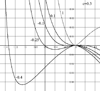
Figure 1: The potential $V_{\rm Ein}(\phi)$ for $d_{1}=3$, $c=0.3$ in the range $\phi>-5/3$, where $F^{\prime}(R)>0$, for a few values of $\Lambda$ (indicated near the curves). The dashed line ($\Lambda=1$) shows a minimum at $\phi=0$. The values of $\varphi$ are expressed in the units $m_{\scriptscriptstyle D}=1$.

In Ref. Zhuk , the authors studied the case $F^{\prime}(R)>0$ and showed analytically that a minimum of the potential stabilizing the extra dimensions is only possible with a negative energy density and a negative curvature $k=-1$. We confirm this result in our approach, see examples in Fig. 1. The energy density corresponding to the minimum value of the potential is negative, which, in the cosmological context, corresponds to anti-de Sitter space-time.

There is one more minimum of the potential $V_{\rm Ein}$ with $F^{\prime}>0$, existing in the range $\Lambda>0$ and located at the point $\phi=0$. The asymptotic $\phi\to 0$ corresponds to growing rather than stabilized extra dimensions: $b={\,\rm e}^{\beta}\sim 1/\sqrt{|\phi|}\to\infty$. A model with such an asymptotic growth at late times may still be of interest if the growth is sufficiently slow and the size $b$ does not reach detectable values by now.

Let us check whether it is possible to describe the modern state of the Universe by an asymptotic form of the solution for $\phi\to 0$ as a spatially flat cosmology with the 4D Einstein-frame metric

$$d{\widetilde{s}}{}^{2}_{4}=dt^{2}-a_{\scriptscriptstyle\rm E}{}^{2}(t)d\vec{x}{}^{2},$$ (40)

where $a_{\scriptscriptstyle\rm E}{}$ is the Einstein-frame scale factor. Two independent components of the Einstein-scalar equations for $\beta(t)$ and $a_{\scriptscriptstyle\rm E}{}(t)$ are

$$\ddot{\beta}+3\frac{{\dot{a}}_{\scriptscriptstyle\rm E}{}}{a_{\scriptscriptstyle\rm E}{}}\dot{\beta} \!= \!\frac{2\Lambda}{d_{1}+1}{\,\rm e}^{-d_{1}\beta},$$

$${}3\frac{{\dot{a}}_{\scriptscriptstyle\rm E}{}^{2}}{a_{\scriptscriptstyle\rm E}{}^{2}} \!= \!\frac{1}{4}d_{1}(d_{1}+1)\dot{\beta}{}^{2}+\Lambda{\,\rm e}^{-d_{1}\beta}.$$ (41)

We seek their solution at large $t$ in the form

$$a_{\scriptscriptstyle\rm E}{}(t)\propto t^{p},\quad\ {\,\rm e}^{\beta}\approx(t/t_{*})^{q},\quad\ p,\ q,\ t_{*}={\rm const}>0,$$ (42)

and find that such a solution does exist with

$${}p=3h,\hskip 28.45274ptq=2/d_{1},$$

$${}h:=\sqrt{(d_{1}+1)/d_{1}},\hskip 28.45274pt\Lambda t_{*}^{2}=h^{2}(9h-1).$$ (43)

Passing over to the Jordan frame with

$$ds^{2}_{4}=d\tau^{2}-a^{2}(\tau)d\vec{x}{}^{2}=\frac{1}{f}\,d{\widetilde{s}}{}^{2}_{4},$$ (44)

due to $F^{\prime}(0)\approx 1$, we can put simply $f={\,\rm e}^{d_{1}\beta}\approx(t/t_{*})^{2}$. We obtain

$$t/t_{*}\propto{\,\rm e}^{\tau/t_{*}},\quad\ a(\tau)\propto{\,\rm e}^{(3h-1)\tau/t_{*}},\quad\ b(\tau)\propto{\,\rm e}^{2\tau/(d_{1}t_{*})}.$$ (45)

The external scale factor $a(\tau)$ grows exponentially, which conforms to modern observations if one properly chooses the constants. The internal scale factor $b(\tau)$ grows much slower for sufficiently large $d_{1}$, but the volume factor $\sim b^{d_{1}}$ grows approximately at the same rate as $a(\tau)$, which means that, e.g., the effective gravitational constant will change too rapidly, at nearly a Hubble rate, contrary to observations. We conclude that the model with $\phi\to 0$ at late times is not very promising.

We have also tried to find minima of the potential in another region, where $F^{\prime}<0$, in a wide range of the parameters $c$ and $\Lambda$.

Some examples of the behavior of the potential for the specific value $c=1.5$ are shown in Fig. 2. Potentials with $\Lambda<0$ show minima with $V_{\min}>0$, so that $\Lambda_{\rm eff}>0$, which should lead to cosmological models with de Sitter external space and stable extra dimensions. Such models again correspond to $\phi<0$, i.e., hyperbolic extra dimensions. By fine tuning of the initial constants $c$ and $\Lambda$ we can obtain the present-day values of the cosmological parameters.

As in Fig. 1, we also find a minimum at $\phi=0$, whose properties have already been discussed.

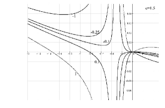
Figure 2: The same as in Fig. 1 but with $c=1.5$. The minima of $V(\phi)$ are situated in the range $\phi<-1/3$, where $F^{\prime}<0$.

We see that the behavior of the system is drastically different in different ranges of $\phi$ and depends on the numerical values of the initial parameters. We also confirm that gravity alone can stabilize the size of extra dimensions, without need for introducing other fields with specific forms of potentials. Positive values of the effective cosmological constant $\Lambda_{\rm eff}$ (vacuum energy density) were found in the range where $F^{\prime}<0$. This is a feature of quadratic gravity only: as will be seen in the next section, e.g., for cubic gravity one may have $\Lambda_{\rm eff}>0$ where $F^{\prime}>0$.

V Other theories

V.1 Cubic gravity

The cubic theory of gravity with

$$F(R)=R+cR^{2}+CR^{3}$$ (46)

is another example of curvature-nonlinear gravity for which Eqs. (II.2) and (17) may be applied. The shape of the potential appears to be very sensitive to the values of the parameters $c$ and $C$. This property may be used to adjust the potentials in such a way that its minimum in the Einstein frame will lead to an extremely small but positive value of $\Lambda_{\rm eff}$ in the Jordan frame, and it turns out that, unlike quadratic gravity, this can be achieved in the range where $F^{\prime}>0$. Examples of such a behavior are shown in Fig. 3. Thus cubic gravity can in principle lead to an appropriate description of our Universe with compact and stable extra dimensions. At large times, when the influence of matter may be neglected compared to the effective cosmological constant, we shall obtain de Sitter expansion of the three observable dimensions.

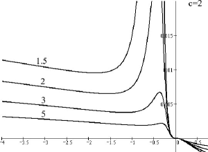
Figure 3: The potential $V_{\rm Ein}$ for cubic gravity with $d_{1}=3$ and $c=2$. The curves are labelled by values of the parameter $C$. Note that $F^{\prime}(\phi)>0$ near the minima.

The range of positive curvature, $\phi>0$, appears to be of lesser interest. It also contains minima but only with $V_{\min}<0$, see Fig. 4. The states in such minima are metastable (since the minima are only local), so that such a space would have a finite lifetime. The latter, however, could be made arbitrarily long by choosing the parameters.

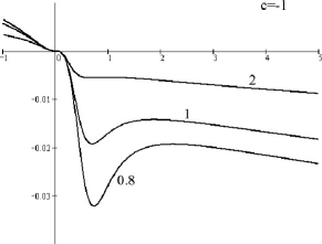
Figure 4: $V_{\rm Ein}(\phi)$ for cubic gravity with $d_{1}=3$, $c=-1$. Lines are labelled by values of the parameter $C$. Again $F^{\prime}(\phi)>0$ near the minima.

V.2 Extensions

The method discussed above allows considering wider classes of Lagrangians. Let us briefly demonstrate this by adding terms proportional to the Ricci tensor squared $R_{AB}R^{AB}$ and the Kretschmann scalar ${\cal K}=R_{ABCD}R^{ABCD}$. By common views, these and other high-order curvature terms appear due to quantum corrections, and it seems natural to include them on equal footing with $cR^{2}$. Now the action has the form

$${}S=\frac{{\cal V}[d_{1}]}{2\varkappa^{2}}\int d^{4}x\,\sqrt{{}^{4}g}{\,\rm e}^{d_{1}\beta}\bigl{(}R+cR^{2}$$

$${}\hskip 28.45274pt+c_{1}R_{AB}R^{AB}+c_{2}{{\cal K}}-2\Lambda\bigr{)},$$ (47)

where the internal variables have been integrated out in full analogy with Eq. (5). For the metric (1), it is easy to obtain expressions for $R_{AB}R^{AB}$ and ${\cal K}$:

$${}R_{AB}R^{AB}={\overline{R}}_{\mu\nu}{\overline{R}}^{\mu\nu}+2d_{1}{\overline{R}}_{\mu\nu}B^{\mu\nu}+{\,\rm e}^{-4\beta}{\overline{R}}_{ab}{\overline{R}}^{ab},$$

$${}\ +2{\,\rm e}^{-2\beta}{\overline{R}}[h][\mathop{\raisebox{-0.5pt}{$\Box$}}\nolimits\beta+d_{1}(\partial{\beta})^{2}]+d_{1}[\mathop{\raisebox{-0.5pt}{$\Box$}}\nolimits\beta+d_{1}(\partial{\beta})^{2}]^{2}$$

(48)

$${}{\cal K}=\overline{{\cal K}}[g]+4d_{1}B_{\mu\nu}B^{\mu\nu}+{\,\rm e}^{-4\beta}\overline{{\cal K}}[h]$$

$${}\qquad+4{\,\rm e}^{-2\beta}{\overline{R}}[h](\partial{\beta})^{2}+2d_{1}(d_{1}-1)[(\partial\beta)^{2}]^{2}.$$ (49)

In the slow-change approximation, in the same manner as in Sec. II, we obtain the 4D effective Lagrangian

$${}\sqrt{{}^{4}g}L=\sqrt{{}^{4}g}{\,\rm e}^{d_{1}\beta}\Big{[}R_{4}(1+2c\phi)+\phi+c_{\rm tot}\phi^{2}-2\Lambda$$

$${}\qquad+(1+2c\phi)f_{1}+2c_{1}\phi\mathop{\raisebox{-0.5pt}{$\Box$}}\nolimits\beta+2(c_{1}d_{1}+2c_{2})(\partial\beta)^{2}\Big{]}$$

with

$$c_{\rm tot}=c+\frac{c_{1}}{d_{1}}+\frac{2c_{2}}{d_{1}(d_{1}-1)}.$$

The conformal mapping (11) leads, after some calculations, to the Einstein-frame Lagrangian (15) with the kinetic and potential terms

$$K_{\rm Ein}(\phi) \!= \!K^{(2)}_{\rm Ein}(\phi)+\frac{c_{1}+c_{2}}{2\phi(1+2c\phi)},$$

$$V_{\rm Ein}(\phi) \!= \!-\mathop{\rm sign}\nolimits(1+2c\phi)$$ (52)

$${}\times\left[\frac{|\phi|}{d_{1}(d_{1}-1)}\right]^{d_{1}/2}\frac{c_{\rm tot}\phi^{2}+\phi-2\Lambda}{(1+2c\phi)^{2}},$$

where the term $K^{(2)}_{\rm Ein}(\phi)$ is taken from (39).

The presence of the parameters $c_{1}$ and $c_{2}$ adds freedom in choosing the shape of the potential. The kinetic term also acquires a more complex form which could significantly affect the field dynamics. Thus, as shown in Ref. Ru04 , zeros of the kinetic term can represent stationary values of $\phi$. It means that a field could be captured in the vicinity of such points in addition to minima of the potential. An analysis of kinetic terms like (V.2) could lead to possibilities of interest, and we hope to return to this point in our future work.

VI Concluding remarks

We have shown that multidimensional gravity alone, even without any fields of non-geometric origin and with a very simple choice of the geometry, can be a basis for rather complicated phenomena. The assumption on nonlinearity of gravity, used in this study, inevitably follows from quantum corrections to the Einstein gravity and must be taken into account for completeness.

We have introduced the slow-change approximation in nonlinear multidimensional gravity, making the analysis easier. This approximation proves to be valid for a wide variety of phenomena where the curvature and energy scales are far from Planckian (though Planckian in a multidimensional sense, which may mean scales different from those known in four-dimensional physics).

Using some simple examples of nonlinear gravity with an arbitrary number of extra dimensions, we have obtained an effective scalar field with quite a complex form of the potential. The kinetic term is also nontrivial and adds complexity to the effective field dynamics. The potentials possess minima, both stable and metastable, thus stabilizing the size of extra dimensions. Some of them seem quite promising for the description of the present state of the Universe with a small positive effective cosmological constant and stable and small enough extra dimensions.

A problem that could not be solved in this paper is that of choosing the observational conformal frame, which is a necessary step in confronting the theory to observations. For our numerical estimates we identified the initial (fundamental) and observational frames. One should, however, bear in mind that it is not the only possible choice, and the right one should follow from a full underlying theory.

The precise number of extra dimensions $d_{1}$ was not very important in our study, and we used the only value $d_{1}=3$ in numerical calculations, though the method is valid for arbitrary $d_{1}$. This number may prove to be more essential in more complex geometries and nonlinear gravity theories.

One of possible applications of this method is the brane world scenario, where, in particular, it opens a direct way of obtaining a stabilizing radion potential instead of postulating it.

Acknowledgment

We thank Julio Fabris for a helpful discussion. KB acknowledges partial financial support from ISTC Project No. 1655 and DFG Project 436RUS113/807/0-1(R).

References

- (1) A.D. Linde, “Particle Physics and Inflationary Cosmology”, Harvard Acad. Press, Geneva (1990).
- (2) D.H. Lyth and E.D. Stewart, “More varieties of hybrid inflation”, Phys. Rev. D 54, 7186–7190 (1996).
- (3) S. Rubin, “Effect of massive fields on inflation”, JETP Lett. 74, 275–279 (2001); hep-ph/0110132.
- (4) On possible variations of the fundamental physical constants see, e.g., the recent reviews: J.-Ph. Uzan, Variation of the constants in the late and early universe, astro-ph/0409424; S.V. Kononogov and V.N. Melnikov, Izmeritel’naya Tekhnika 6, 1 (2005), and numerous references therein.
- (5) R. Holman, E.W. Kolb, S.I. Vadas and Y. Wang, “Extended inflation from higher-dimensional theories”, Phys. Rev. D 43, 995 (1991).
- (6) A.S. Mazumdar and S.K. Sethi, “Extended inflation from Kaluza-Klein theories”, Phys. Rev. D 46, 5315-5320 (1992).
- (7) A.A. Grib, S.G. Mamaev and V.M. Mostepanenko, “Quantum Effects in Strong External Fields”, Atomizdat, Moscow, 1980 (in Russian).
- (8) N. Birrell and P. Davies, “Quantum Fields in Curved Space”, Cambridge Univ. Press, 1982.
- (9) John F. Donoghue, Phys. Rev. D 50, 3874-3888 (1994).
- (10) A. Starobinsky, “A new type of isotropic cosmological models without singularity”, Phys. Lett. 91B, 99–102 (1980).
- (11) M. Malquarti, E.J. Copeland, A.R. Liddle and M. Trodden, “A new view of k-essence”, Phys. Rev. D 67, 123503 (2003); astro-ph/0302279.
- (12) K.A. Bronnikov and V.N. Melnikov, “Conformal frames and D-dimensional gravity”, gr-qc/0310112, in: Proceedings of the 18th Course of the School on Cosmology and Gravitation: The Gravitational Constant. Generalized Gravitational Theories and Experiments (30 April-10 May 2003, Erice), Ed. G.T. Gillies, V.N. Melnikov and V. de Sabbata, Kluwer, Dordrecht/Boston/London, 2004, pp. 39–64.
- (13) H. Kroger, G. Melkonian and S.G. Rubin, “Singular points in scalar-tensor theory”, Gen. Rel. Grav. 36, 1649 (2004); astro-ph/0310182.
-
(14)
U. Günther, P. Moniz and A. Zhuk, “Multidimensional cosmology and
asymptotical ADS”, Astrophys. Space Sci. 283, 679-684
(2003); gr-qc/0209045;
U. Günther and A. Zhuk, “Remarks on dimensional reduction in multidimensional cosmological models”, gr-qc/0401003. - (15) Compact hyperbolic spaces of constant curvature on the basis of a usual open Lobachevsky space are isometric to quotient spaces where is a nontrivial discrete group of isometries of , see, e.g., B.A. Dubrovin, A.T. Fomenko and S.P. Novikov, “Modern Geometry — Methods and Applications”, Springer-Verlag, New York, 1992. On possible applications of such (3D) spaces in cosmology see, e.g., D. Müller, H.V. Fagundes and R. Opher, Phys. Rev. D 66, 083507 (2002) and references therein.
-
(16)
R. Kerner, Gen. Rel. Grav. 14, 453 (1982);
J.D. Barrow and A.C. Ottewill, J. Phys. A 10, 2757 (1983);
J.P. Duruisseu and R. Kerner, Gen. Rel. Grav. 15, 797 (1983);
B. Whitt, Phys. Lett. 145B, 176 (1984);
J.D. Barrow and S. Cotsakis, Phys. Lett. 214B, 515 (1988);
K. Maeda, J.A. Stein-Schabes and T. Futamase, Phys. Rev. D 39, 2848 (1989);
G. Magnano and L.M. Sokolowski, Phys. Rev. D 50, 5039 (1994), gr-qc/9312008;
J. Ellis, N. Kaloper, K.A. Olive and J. Yokoyama, Phys. Rev. D 59, 103503 (1999), hep-ph/9807482. - (17) K. Maeda, Phys. Rev. D 39, 3159 (1989).
- (18) R. Wagoner, Phys. Rev. D 1, 3209 (1970).
- (19) K.A. Bronnikov, “Scalar-tensor gravity and conformal continuations”, J. Math. Phys. 43, 6096–6115 (2002); gr-qc/0204001.
- (20) K.A. Bronnikov and M.S. Chernakova, “ theory of gravity and conformal continuations”, Izv. Vuzov, Fiz. No. 9, 46 (2005); Russ. Phys. J. 48, 940 (2005); gr-qc/0503025.
-
(21)
K.A. Bronnikov and Yu.N. Kireyev,
“Instability of black holes with scalar charge”,
Phys. Lett. 67A, 95 (1978);
A.A. Starobinsky, Pis’ma v Astron. Zh. 7, 67 (1981); Sov. Astron. Lett. 7, 361 (1981);
K.A. Bronnikov and S.V. Grinyok, “Conformal continuations and wormhole instability in scalar-tensor gravity”, Grav. & Cosmol. 10, 237–244 (2004), gr-qc/0411064; Grav. & Cosmol. 11, 75–81 (2005), gr-qc/0509062.