Potential symmetry and invariant solutions of Fokker-Planck equation in

cylindrical coordinates related to magnetic field diffusion

in magnetohydrodynamics including the Hall current

A. H. Khater^a,1, D. K. Callebaut^b, S. F. Abdul-Aziz^a,

T. N. Abdelhameed^a

^aDepartement of Mathematics, Faculty of Science, Beni-Suef University, Beni-Suef, Egypt

^bDepartement Natuurkunde, CDE, University of Antwerp, B-2610 Antwerp, Belgium

Abstract

Lie groups involving potential symmetries are applied in connection with the system of magnetohydrodynamic equations for incompressible matter with Ohm’s law for finite resistivity and Hall current in cylindrical geometry. Some simplifications allow to obtain a Fokker-Planck type equation. Invariant solutions are obtained involving the effects of time-dependent flow and the Hall-current. Some interesting side results of this approach are new exact solutions that do not seem to have been reported in the literature.

PACS: 02.Jr; 05.10.Gg; 52.30.Cv; 52.Ff

Keywords: Magnetohydrodynamics; Dissipative systems; Hall-current; Fokker-Planck type equations; Exact solutions.

1 Introduction

Recently, Khater et al. [1, 2] have analyzed the generalized one-dimensional Fokker-Planck (FP) equation and the inhomogeneous NL diffusion equation through the application of the potential symmetries. For a brief exposition of the potential symmetries and of the equations of magnetohydrodynamics (MHD): see [2].

Some interesting side results of the present study are new exact solutions that do not seem to have been reported in the literature.

This paper is organized as follows:

Section 2 deals with the determination of the potential symmetries. In section 3, we analyze the invariant solutions of the MHD equations for various cases corresponding to physically interesting situations. Section 4 gives the conclusions.

2 Determination of the potential symmetries

Consider a partial differential equation (PDE), $R$, of order m written in a conserved form: ( [3] and references therein)

$$\sum^{n}_{i=1}\frac{\partial}{\partial x_{i}}F_{i}[x,u,u_{1},u_{2},...,u_{m-1}]=0$$ (2.1)

with $n\geq 2$ independent variables $x=(x_{1},x_{2},...,x_{n})$ and a single dependent variable $u$. For simplicity, we consider a single PDE - the generalization to a system of PDEs in a conserved form is straight-forward. The indexes of $u$ indicate the order of the derivative. If a given PDE is not written in a conserved form, there are a number of ways of attempting to put it in a conserved form. These include a change of variables (dependent as well as independent), an application of Noether’s theorem [4], direct construction of conservation laws from field equations [5], and some combinations of them.

Using some simplifications [2] we may put the equation of the evolution of flow in the MHD system for cylindrical coordinates, which is a generalized FP equation, in the following conservative form:

$$u_{t}-(\frac{1}{r^{2}}u_{\theta}+\frac{1}{r}\lambda_{t}\theta u)_{\theta}=0$$ (2.2)

with $\lambda$ a function of $r$ and $t$; By considering a potential $v$ as an auxiliary unknown function, the following system $S$ can be associated with (2.2):

$$v_{\theta}=u\quad,\quad v_{t}=\frac{1}{r^{2}}u_{\theta}+\frac{1}{r}\lambda_{t}\theta u.$$ (2.3)

It is well known that the homogeneous linear system, which characterizes the generators, is obtained from [6]

$$Y^{(1)}(v_{\theta}-u)|_{s}=0\quad,\quad Y^{(1)}(v_{t}-\frac{1}{r^{2}}u_{\theta}-\frac{1}{r}\lambda_{t}\theta u)|_{s}=0$$ (2.4)

which must hold identically.

Here, $Y^{(1)}$ is the operator:

$$Y^{(1)}=\tau\frac{\partial}{\partial t}+\xi\frac{\partial}{\partial\theta}+\eta\frac{\partial}{\partial u}+\phi\frac{\partial}{\partial v}+\eta^{(1)}_{1}\frac{\partial}{\partial u_{t}}+\eta^{(1)}_{2}\frac{\partial}{\partial u_{\theta}}+\phi^{(1)}_{1}\frac{\partial}{\partial v_{t}}+\phi^{(1)}_{2}\frac{\partial}{\partial v_{\theta}};$$ (2.5)

$$\begin{split}\eta^{(1)}_{1}&=\eta_{t}+(\eta_{u}-\tau_{t})u_{t}-\tau_{u}u^{2}_{t}-\xi_{t}u_{\theta}-\xi_{u}u_{t}u_{\theta}+\eta_{v}v_{t}-\tau_{v}u_{t}v_{t}-\xi_{v}u_{\theta}v_{t},\\ \eta^{(1)}_{2}&=\eta_{\theta}+(\eta_{u}-\xi_{\theta})u_{\theta}-\tau_{\theta}u_{t}-\tau_{u}u_{\theta}u_{t}-\xi_{u}u^{2}_{\theta}+\eta_{v}v_{\theta}-\tau_{v}u_{t}v_{\theta}-\xi_{v}u_{\theta}v_{\theta},\\ \phi^{(1)}_{1}&=\phi_{t}+(\phi_{v}-\tau_{t})v_{t}-\tau_{v}v^{2}_{t}+\phi_{u}u_{t}-\tau_{u}u_{t}v_{t}-\xi_{t}v_{\theta}-\xi_{u}u_{t}v_{\theta}-\xi_{v}v_{t}v_{\theta},\\ \phi^{(1)}_{2}&=\phi_{\theta}+(\phi_{v}-\xi_{\theta})v_{\theta}-\xi_{v}v^{2}_{\theta}+\phi_{u}u_{\theta}-\tau_{\theta}v_{t}-\tau_{u}u_{\theta}v_{t}-\tau_{v}v_{\theta}v_{t}-\xi_{u}u_{\theta}v_{\theta}\end{split}$$

Eq. (2.4) becomes

$$\phi_{\theta}+(\phi_{v}-\xi_{\theta})v_{\theta}-\xi_{v}v^{2}_{\theta}+\phi_{u}u_{\theta}-\tau_{\theta}v_{t}-\tau_{u}u_{\theta}v_{t}-\tau_{v}v_{\theta}v_{t}-\xi_{u}u_{\theta}v_{\theta}-\eta=0,$$ (2.6)

$$\begin{split}\phi_{t}&+(\phi_{v}-\tau_{t})v_{t}-\tau_{v}v^{2}_{t}+\phi_{u}u_{t}-\tau_{u}u_{t}v_{t}-\xi_{t}v_{\theta}-\xi_{u}u_{t}v_{\theta}\\ &-\xi_{v}v_{t}v_{\theta}-\frac{1}{r}\lambda_{t}\theta\eta-\frac{1}{r}\lambda_{t}u\xi-\frac{1}{r^{2}}[\eta_{\theta}+(\eta_{u}-\xi_{\theta})u_{\theta}-\tau_{\theta}u_{t}\\ &-\tau_{u}u_{\theta}u_{t}-\xi_{u}u^{2}_{\theta}+\eta_{v}v_{\theta}-\tau_{v}u_{t}v_{\theta}-\xi_{v}u_{\theta}v_{\theta}]-\frac{1}{r}\theta\lambda_{tt}\tau u=0\end{split}$$ (2.7)

On substituting $v_{\theta}$ by $u$, and $v_{t}$ by $\frac{1}{r^{2}}u_{\theta}+\frac{1}{r}\lambda_{t}\theta u$ in Eqs. (2.6) and (2.7), we get:

$$\tau=\tau(t)\quad,\quad\xi=\xi(\theta,t)\quad,\quad\phi_{u}=0$$ (2.8)

$$\phi_{\theta}-\eta+(\phi_{v}-\xi_{\theta})u=0$$ (2.9)

$$\phi_{v}-\eta_{u}-\tau_{t}+\xi_{\theta}=0$$ (2.10)

$$\phi_{t}-\frac{1}{r^{2}}\eta_{\theta}-\frac{1}{r}\lambda_{t}\theta\eta+[\frac{1}{r}\lambda_{t}\theta(\phi_{v}-\tau_{t})-\frac{1}{r}\lambda_{t}\xi-\xi_{t}-\frac{1}{r^{2}}\eta_{v}+\frac{1}{r}\lambda_{tt}\theta\tau]u=0;$$ (2.11)

with

$$\eta=f(\theta,t)u+g(\theta,t)v\quad,\quad\phi=k(\theta,t)v,$$ (2.12)

where $f,g$ and $k$ are arbitrary smooth functions of $\theta$ and $t$.

On solving the above system of Eqs. (2.8)-(2.12), we get:

$$\tau=\tau(t)\quad,\quad\xi=\xi(\theta,t),$$ (2.13)

$$k_{\theta}-g=0,$$ (2.14)

$$K-f-\xi_{\theta}=0,$$ (2.15)

$$2\xi_{\theta}-\tau_{t}=0$$ (2.16)

$$k_{t}-\frac{1}{r^{2}}g_{\theta}-\frac{1}{r}\lambda_{t}\theta g=0,$$ (2.17)

$$\frac{1}{r}\lambda_{t}\theta\tau+\frac{1}{r^{2}}g+\frac{1}{r^{2}}f_{\theta}+\xi_{t}+\frac{1}{r}\theta\lambda_{t}\xi_{\theta}+\frac{1}{r}\lambda_{t}\xi=0,$$ (2.18)

$$g_{t}=(\frac{1}{r^{2}}g_{\theta}+\frac{1}{r}\lambda{t}\theta g)_{\theta}.$$ (2.19)

In solving the above system of Eqs.(2.13)-(2.19), we confine our attention to physically interesting situations.

3 Invariant solutions

From now on, we will denote by $c_{0}-c_{13}$ arbitrary constants

Let $\lambda=\frac{1}{2r}$

In this case, the infinitesimal symmetries are given by :

$$\left.\begin{split}\tau&=-2r^{2}c_{4}e^{-\frac{t}{r^{2}}}+c_{5},\\ \xi&=c_{4}e^{-\frac{t}{r^{2}}}\theta+c_{3}e^{-\frac{t}{2r^{2}}}-2\sqrt{2r}c_{0}e^{\frac{t}{2r^{2}}},\\ \eta&=(\sqrt{2r}c_{0}e^{\frac{t}{2r^{2}}}\theta+c_{1}-c_{2})u+\sqrt{2r}c_{0}e^{\frac{t}{2r^{2}}}v,\\ \phi&=(\sqrt{2r}c_{0}e^{\frac{t}{2r^{2}}}\theta+c_{1})v\end{split}\right\}$$ (3.1)

Then, we obtain point symmetries with the following generators :

$$\begin{split}Y_{1}&:\tau=0,\quad\xi=-2\sqrt{2r}e^{\frac{t}{2r^{2}}},\quad\eta=\sqrt{2r}e^{\frac{t}{2r^{2}}}\theta u+\sqrt{2r}e^{\frac{t}{2r^{2}}}v,\quad\phi=\sqrt{2r}e^{\frac{t}{2r^{2}}}\theta v,\\ Y_{2}&:\tau=\xi=0,\quad\eta=u,\quad\phi=v,\\ Y_{3}&\tau=\xi=\phi=0,\quad\eta=-u,\\ Y_{4}&:\tau=\eta=\phi=0,\quad\xi=e^{-\frac{t}{r^{2}}}\\ Y_{5}&:\tau=-2r^{2}e^{-\frac{t}{r^{2}}},\quad\xi=e^{-\frac{t}{r^{2}}}\theta,\quad\eta=\phi=0,\\ Y_{6}&:\tau=1,\quad\eta=\phi=\xi=0\end{split}$$

and $\infty$-dimensional symmetry, which is a consequence of the linearity [7]. It is clear that, $Y_{1}$ is only a potential symmetry for Eq.(2.2).

For the potential symmetry $Y_{1}$, the characteristic system related to the invariant surface conditions reads:

$$v=c_{7}e^{\frac{-\theta^{2}}{4}},\qquad t=c_{6}$$ (3.2)

$$u=(c_{8}-\frac{c_{7}}{2}\theta)e^{\frac{-\theta^{2}}{4}}$$ (3.3)

If we assume $t=c_{6}=z$ as a parameter, $c_{7}=h_{2}(z)$, and $c_{8}=h_{1}(z)$ in Eqs. (3.2) and (3.3), we obtain:

$$u=(h_{1}(z)-\frac{h_{2}(z)}{2}\theta)e^{\frac{-\theta^{2}}{4}},$$ (3.4a)

$$v=h_{2}(z)e^{\frac{-\theta^{2}}{4}};\quad z=t$$ (3.4b)

Now, to find the solutions $F^{*}_{E}$, we introduce Eq. (3.4a) in Eq. (2.2) obtaining:

$$h^{{}^{\prime}}_{1}-\theta(\frac{h^{{}^{\prime}}_{2}}{2}+\frac{h_{2}}{4r^{2}})=0$$ (3.5)

which must hold for any value of $\theta$.

From Eq. (3.5), we have the system $\overset{=}{\varphi}$ as:

$$\left.\begin{split}h^{{}^{\prime}}_{1}&=0,\\ \frac{h^{{}^{\prime}}_{2}}{2}+\frac{h_{2}}{4r^{2}}&=0\end{split}\right\}$$ (3.6)

which on solving, yields

$$\left.\begin{split}h_{1}(z)&=c_{9},\\ h_{2}(z)&=c_{10}e^{-\frac{t}{2r^{2}}}\end{split}\right\}$$ (3.7)

Then, the family $F^{*}_{E}$ is therefore:

$$u=(c_{9}-\frac{c_{10}}{2}\theta e^{-\frac{t}{2r^{2}}})e^{-\frac{\theta^{2}}{4}}$$ (3.8)

Also, Eq. (3.4a) is a family of solutions of the first-order equation:

To find the solutions $F_{E}$, we introduce Eq. (3.4) in Eq. (2.3) obtaining the system $\overset{=}{\varphi}$ as:

$$\left.\begin{split}h_{1}&=0,\\ h^{{}^{\prime}}_{2}+\frac{h_{2}}{2r^{2}}&=0\end{split}\right\}$$ (3.9)

which on solving, yields

$$\left.\begin{split}h_{1}(z)&=0,\\ h_{2}(z)&=c_{11}e^{-\frac{t}{2r^{2}}}\end{split}\right\}$$ (3.10)

Then, the family $F_{E}$ is therefore:

$$u=-\frac{c_{11}}{2}\theta e^{-\frac{1}{4r^{2}}(\theta^{2}r^{2}+2t)}\quad(\text{see fig. (2)}).$$ (3.11)

It is clear that, $F_{E}$ is enclosed in $F^{*}_{E}$, which are new solutions as far as we know.

Particular case.

If, $f=\lambda_{t}\theta$, $g=v^{z}=0$, and $u=\Theta_{\theta}$ in Eqs. (2.10)-(2.13) we obtain that

$$f_{1}(t)=0,$$ (3.12)

$$u=u(t)$$ (3.13)

$$u_{t}=\frac{1}{r}\lambda_{t}u,$$ (3.14)

$$\lambda_{tt}+\frac{2}{r}\lambda^{2}-\frac{1}{r^{2}}\lambda=0\qquad\upsilon_{m}=1$$ (3.15)

Solving Eq. (3.15), yields

$$\lambda_{t}=\frac{1}{2r+c_{12}e^{-\frac{t}{r^{2}}}}$$ (3.16)

Then, the family $F^{*}_{E}$ is given by:

$$u=c_{13}\sqrt{2re^{\frac{t}{r^{2}}}+c_{12}}\quad(\text{see fig. (3)}).$$ (3.17)

It is clear that, $F_{E}$ is enclosed in $F^{*}_{E}$, which are new solutions as far as we know.

4 Conclusion

In this paper, we made an analysis for the FP-type equation with convection given by the plasma flow with finite electrical conductivity and Hall current. This method based on potential symmetries turns out to be an alternative, systematic and powerful technique for the determination of the solutions of linear or nonlinear PDEs, single or a system. The infinitesimals, similarity variables, dependent variables, and reduction to quadrature or exact solutions of the mentioned FP-type equation (in cylindrical coordinates) for physically realizable forms of $\lambda$, and $q$ are also obtained.

The similarity solutions given here do not seem to have been reported in the literature. Some of these solutions are unbounded. However, one can deal with them as various methods have been elaborated to analyze the properties of unbounded (particularly explosive type) solutions of the Cauchy problem of quasilinear parabolic equations of type (2.2).

References

[1] A. H. Khater, M. H. M. Moussa, S. F. Abdul-Aziz, Physica A 304 (2002) 395.

[2] A. H. Khater, D. K. Callebaut, S. F. Abdul-Aziz, T. N. Abdelhameed, Physica A., 341 (2004) 107.

[3] G. W. Bluman, S. Kumei, G.J. Reid, J. Math. Phys. 29 (1988) 806.

[4] J. D. Logan, Invariant Variational Principles, Academic Press, New York, 1977.

[5] S. C. Anco, G. W. Bluman, Phys. Rev. Lett. 78 (1997) 2869.

[6] G. W. Bluman, J. D. Cole, Similarity Methods for Differential Equations (Springer-Verlag, New York, 1974).

[7] G. W. Bluman, S. Kumei, Symmetries and Differential Equations, Springer-Verlag, New York, 1989.

Figure Captions :

Fig. (1a): The magnetic field in the surface with $\mu_{1}=10,\mu_{2}=0.1$ and $m=0.001$

Fig. (1b): The magnetic field in the surface with $\mu_{1}=-10,\mu_{2}=0.1$ and $m=0.001$

Fig. (1c): The magnetic field in the surface with $\mu_{1}=10,\mu_{2}=0$ and $m=0.01$

Fig. (2a): The solution for a Fokker-Planck in the surface with $c_{11}=-30$, $t=0$

Fig. (2b): The solution for a Fokker-Planck in the surface with $c_{11}=-30$, $t=1$

Fig. (2c): The solution for a Fokker-Planck in the surface with $c_{11}=30$, $t=1$

Fig. (3a) : The solution for a Fokker-Planck in the surface with (particular case) $c_{13}=5$, $t=0$, $c_{12}=1$

Fig. (3b) : The solution for a Fokker-Planck in the surface with (particular case) $c_{13}=5$, $t=1$, $c_{12}=1$

Fig. (3c) : The solution for a Fokker-Planck in the surface with (particular case) $c_{13}=5$, $t=2$, $c_{12}=-10$

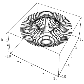
Figure 1: fig (1a)

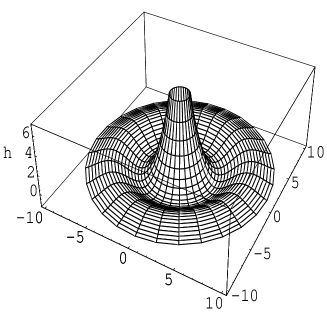
Figure 2: fig (1b)

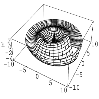
Figure 3: fig (1c)

Figure 4: fig (2a)

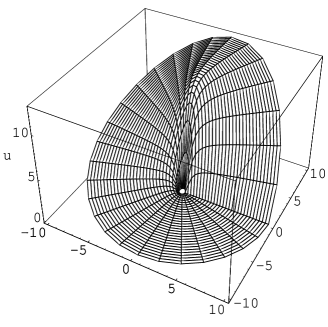
Figure 5: fig (2b)

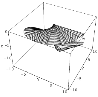
Figure 6: fig (2c)

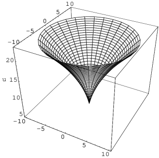
Figure 7: fig (3a)

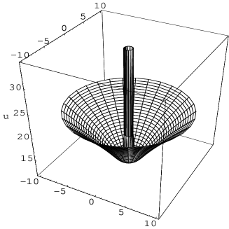
Figure 8: fig (3b)

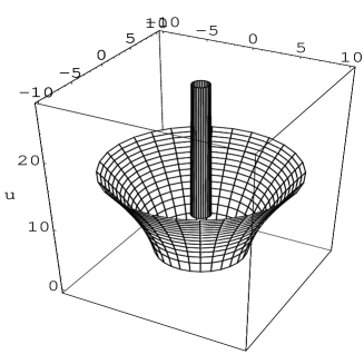
Figure 9: fig (3c)