A radiometer for stochastic gravitational waves

Abstract

The LIGO Scientific Collaboration recently reported a new upper limit on an isotropic stochastic background of gravitational waves obtained based on the data from the 3rd LIGO science Run (S3). Now I present a new method for obtaining directional upper limits that the LIGO Scientific Collaboration intends to use for future LIGO science runs and that essentially implements a gravitational wave radiometer.

.

1 Introduction

The LIGO Scientific Collaboration analyzed the data from the 3rd LIGO science run (S3) looking for an isotropic background of gravitational waves. In Ref. [1] it was reported that a 90%-confidence Bayesian upper limit on $\Omega_{\rm gw}(f)$ of $8.4\times 10^{-4}$ was achieved. $\Omega_{\rm gw}(f)$ is the energy density per logarithmic frequency interval associated with gravitational waves normalized by the critical energy density $\rho_{c}$ to close the universe. However it is possible that the dominant source of stochastic gravitational waves in the LIGO frequency band comes from an ensemble of astrophysical sources (e.g. [3, 4]). If such an ensemble also turns out to be dominated by its strongest members the assumption of isotropy is no longer very good. Then one should look for anisotropies in the stochastic gravitational wave background. This was addressed in Ref. [5, 6], but they focused on getting optimal estimates for each spherical harmonic. If the stochastic gravitational wave background is indeed dominated by individual sources one can get a better signal-to-noise ratio by obtaining optimal filters for small patches of the sky.

I present such a directional method that essentially implements a gravitational wave radiometer. The algorithm has been implemented and will be used to analyze future LIGO science runs starting with S4.

2 Search for an isotropic background

The data from the first 3 LIGO science runs was analyzed with a method described in detail in Ref. [7, 1, 2]. The data streams from a pair of detectors were cross-correlated with a cross-correlation kernel $Q$ chosen to be optimal for an assumed strain power spectrum $H(f)\!=\!H(|f|)$ and angular distribution $P({\hat{\Omega}})\!=\!1$ (isotropic distribution). Specifically, with $S_{1}(f)$ and $S_{2}(f)$ representing the Fourier transforms of the strain outputs of two detectors, this cross-correlation is computed in frequency domain segment by segment as:

$$Y=\int_{-\infty}^{\infty}df\ \int_{-\infty}^{\infty}df^{\prime}\delta_{T}(f-f^{\prime})\,S_{1}^{*}(f)\,Q(f^{\prime})\,S_{2}(f^{\prime})$$ (1)

where $\delta_{T}$ is a finite-time approximation to the Dirac delta function. The optimal filter $Q$ has the form:

$$Q(f)=\lambda\frac{\gamma_{\rm iso}(f)H(f)}{P_{1}(f)P_{2}(f)}$$ (2)

where $\lambda$ is a normalization factor, $P_{1}$ and $P_{2}$ are the strain noise power spectra of the two detectors, $H(f)$ is the strain power spectrum of the stochastic background being searched for ($=S_{\rm gw}(f)$ in Ref. [1, 2]) and the factor $\gamma_{\rm iso}$ takes into account the cancellation of an isotropic omni-directional signal ($P({\hat{\Omega}})\!=\!1$) at higher frequencies due to the detector separation. $\gamma_{\rm iso}$ is called the overlap reduction function [8] and is given by (the normalization is such that $\gamma_{\rm iso}(f\!=\!0)\!=\!1$ for aligned and co-located detectors):

$$\gamma_{\rm iso}(f)=\frac{5}{8\pi}\sum_{A}\int_{S^{2}}d{\hat{\Omega}}\,\,e^{i2\pi f{\hat{\Omega}}\cdot\frac{{\Delta\!\!\stackrel{{\scriptstyle\rightharpoonup}}{{x}}}}{c}}\,\,F_{1}^{A}({\hat{\Omega}})F_{2}^{A}({\hat{\Omega}})$$ (3)

where ${\Delta\!\!\stackrel{{\scriptstyle\rightharpoonup}}{{x}}}={\stackrel{{\scriptstyle\rightharpoonup}}{{x}}}_{2}-{\stackrel{{\scriptstyle\rightharpoonup}}{{x}}}_{1}$ is the detector separation vector and

$$F_{i}^{A}({\hat{\Omega}})=e_{ab}^{A}({\hat{\Omega}})\frac{1}{2}(\hat{X}_{i}^{a}\hat{X}_{i}^{b}-\hat{Y}_{i}^{a}\hat{Y}_{i}^{b})$$ (4)

is the response of detector i to a zero frequency, unit amplitude, $A=+,\times$ polarized gravitational wave.

The optimal filter $Q$ is derived assuming that the intrinsic detector noise is Gaussian and stationary over the measurement time, uncorrelated between detectors, and uncorrelated with and much greater in power than the stochastic gravitational wave signal. Under these assumptions the expected variance, $\sigma^{2}_{Y}$, of the cross-correlation is dominated by the noise in the individual detectors, whereas the expected value of the cross-correlation $Y$ depends on the stochastic background power spectrum:

$$\sigma_{Y}^{2}\equiv\langle Y^{2}\rangle-\langle Y\rangle^{2}\approx\frac{T}{4}\left(Q,Q\right)\>,\,\,\,\,\,\,\,\,\,\,\,\,\langle Y\rangle=T\left(Q,\frac{\gamma_{\rm iso}H}{P_{1}P_{2}}\right)$$ (5)

Here the scalar product $\left(\cdot,\cdot\right)$ is defined as $\left(A,B\right)=\int_{-\infty}^{\infty}A^{*}(f)B(f)P_{1}(f)P_{2}(f)df$ and $T$ is the duration of the measurement.

To deal with the long-term non-stationarity of the detector noise the data set from a given interferometer pair is divided into equal-length intervals, and the cross-correlation $Y$ and theoretical $\sigma_{Y}$ are calculated for each interval, yielding a set $\{Y_{I},\sigma_{Y_{I}}\}$ of such values, with $I$ labeling the intervals. The interval length can be chosen such that the detector noise is relatively stationary over one interval. In Ref. [1, 2] the interval length was chosen to be 60 sec. The cross-correlation values are combined to produce a final cross-correlation estimator, $Y_{\rm opt}$, that maximizes the signal-to-noise ratio, and has variance $\sigma_{\rm opt}^{2}$:

$$\begin{array}[]{cc}Y_{\rm opt}=\sum_{I}\sigma_{Y_{I}}^{-2}Y_{I}/\sigma_{\rm opt}^{-2}\ ,&\,\,\,\,\,\,\,\,\,\,\,\,\sigma_{\rm opt}^{-2}=\sum_{I}\sigma_{Y_{I}}^{-2}\ .\end{array}$$ (6)

Since the LIGO Hanford and Livingston sites are separated by 3000km the overlap reduction function for this pair has already dropped below 5% around each interferometer’s sweet spot of 150 Hz. One unfortunate drawback of this analysis thus is the limited use it makes of the individual interferometer’s most sensitive frequency region. Moreover, if the dominant gravitational wave background would be of astrophysical origin the assumption of an isotropic background is not well justified. If for example the signal is dominated by a few strong sources a directed search can achieve a better signal-to-noise ratio.

3 Directional search: a gravitational wave radiometer

A natural generalization of the method described above can be achieved by finding the optimal filter for an angular power distribution $P({\hat{\Omega}})$. In this case Eq. 5b generalizes to

$$\langle Y\rangle=T\left(Q,\frac{\int_{S^{2}}d{\hat{\Omega}}\gamma_{{\hat{\Omega}}}P({\hat{\Omega}})H}{P_{1}P_{2}}\right)$$ (7)

where $\gamma_{{\hat{\Omega}}}$ is now just the integrand of $\gamma_{\rm iso}$, i.e.

$$\gamma_{{\hat{\Omega}}}=\frac{1}{2}\sum_{A}e^{i2\pi f{\hat{\Omega}}\cdot\frac{{\Delta\!\!\stackrel{{\scriptstyle\rightharpoonup}}{{x}}}}{c}}\,\,F_{1}^{A}({\hat{\Omega}})F_{2}^{A}({\hat{\Omega}})$$ (8)

and $H(f)$ is the strain power spectrum of an unpolarized point source, summed over both polarizations. Note that $\gamma_{{\hat{\Omega}}}$ also becomes sidereal time dependent both through ${\Delta\!\!\stackrel{{\scriptstyle\rightharpoonup}}{{x}}}$ and $F_{i}^{A}({\hat{\Omega}})$.

Eq. 7 was used in Ref. [5] as a starting point to derive optimal filters for each spherical harmonic. However if one wants to optimize the method for well located astrophysical sources it seems more natural to use a $P({\hat{\Omega}})$ that only covers a localized patch in the sky. Indeed, for most reasonable choices of $H(f)$, the resulting maximal resolution of this method will be bigger than a several tens of square degrees such that most astrophysical sources won’t be resolved. Therefore it makes sense to optimize the method for true point sources, i.e. $P({\hat{\Omega}})=\delta^{2}({\hat{\Omega}},{\hat{\Omega}}^{\prime})$.

With this choice of $P({\hat{\Omega}})$ the optimal filter $Q_{{\hat{\Omega}}^{\prime}}$ for the sky direction ${\hat{\Omega}}^{\prime}$ becomes

$$Q_{{\hat{\Omega}}^{\prime}}(f)=\lambda\frac{\gamma_{{\hat{\Omega}}^{\prime}}(f)H(f)}{P_{1}(f)P_{2}(f)}$$ (9)

and the expected cross-correlation $Y_{{\hat{\Omega}}^{\prime}}$ and its expected variance $\sigma^{2}_{Y_{{\hat{\Omega}}^{\prime}}}$ are

$$\sigma_{Y_{{\hat{\Omega}}^{\prime}}}^{2}\equiv\langle Y^{2}_{{\hat{\Omega}}^{\prime}}\rangle-\langle Y_{{\hat{\Omega}}^{\prime}}\rangle^{2}\approx\frac{T}{4}\left(Q_{{\hat{\Omega}}^{\prime}},Q_{{\hat{\Omega}}^{\prime}}\right)\>,\,\,\,\,\,\,\,\,\,\,\,\,\langle Y_{{\hat{\Omega}}^{\prime}}\rangle=T\left(Q_{{\hat{\Omega}}^{\prime}},\frac{\gamma_{{\hat{\Omega}}^{\prime}}H}{P_{1}P_{2}}\right)$$ (10)

3.1 Integration over sidereal time

Since the non-stationarity of the detector noise also needs to be dealt with, processing the data on a segment by segment basis still makes sense. However $\gamma_{{\hat{\Omega}}}$ changes with sidereal time. By setting it to its mid-segment value one can get rid of the 1st order error, but a 2nd order error remains and is of the order

$$Y_{\rm err}(T_{\rm seg})/Y=\frac{{T_{\rm seg}}^{2}}{12}\frac{\int_{-\infty}^{\infty}\frac{\partial^{2}\gamma_{{\hat{\Omega}}^{\prime}}^{*}}{\partial t^{2}}\gamma_{{\hat{\Omega}}^{\prime}}\frac{H^{2}}{P_{1}P_{2}}df}{\int_{-\infty}^{\infty}\gamma_{{\hat{\Omega}}^{\prime}}^{2}\frac{H^{2}}{P_{1}P_{2}}df}=O\left(\left(\frac{2\pi fd}{c}\frac{T_{\rm seg}}{1~{}{\rm day}}\right)^{2}\right)$$ (11)

with $f$ the typical frequency and $d$ the detector separation. For $T_{\rm seg}=60~{}{\rm sec}$, $f=2~{}{\rm kHz}$ and $d=3000~{}{\rm km}$ this error is less than 1%.

Thus the integration over sidereal time for each ${\hat{\Omega}}^{\prime}$ again reduces to the optimal combination of the set $\{Y_{I},\sigma_{Y_{I}}\}_{{\hat{\Omega}}^{\prime}}$ given by Eq. 6. The only difference to the isotropic $P({\hat{\Omega}})\!=\!1$ case is that the optimal filter $Q_{{\hat{\Omega}}^{\prime}}$ is different for each interval $I$ and each sky direction ${\hat{\Omega}}^{\prime}$.

3.2 Numerical aspects

To implement this method one thus has to calculate

$$Y_{{\hat{\Omega}}^{\prime}}=\lambda T\int_{-\infty}^{\infty}df\frac{\gamma_{{\hat{\Omega}}^{\prime}}^{*}H}{P_{1}P_{2}}S1^{*}S2\>,\,\,\,\,\,\,\,\,\,\,\,\,\sigma_{{\hat{\Omega}}^{\prime}}^{2}=\lambda^{2}\frac{T}{4}\int_{-\infty}^{\infty}df\frac{|\gamma_{{\hat{\Omega}}^{\prime}}|^{2}H^{2}}{P_{1}P_{2}}$$ (12)

for each sky direction ${\hat{\Omega}}^{\prime}$ and each segment $I$. This can be calculated very efficiently by realizing that $\gamma_{{\hat{\Omega}}}$ splits into a DC part ${1}/{2}\sum_{A}F_{1}^{A}({\hat{\Omega}})F_{2}^{A}({\hat{\Omega}})$ and a phasor $\exp({i2\pi f{\hat{\Omega}}\cdot{{\Delta\!\!\stackrel{{\scriptstyle\rightharpoonup}}{{x}}}}/{c}})$. For both integrals the DC part can be taken out of the frequency integration, leaving all the directional information of the integrands in the phasor. Thus, with $N$ the number of sky directions ${\hat{\Omega}}^{\prime}$, instead having to calculate $2N$ integrations, it is sufficient to calculate one fast Fourier transform and one integral per segment, and read out the cross-correlation $Y_{{\hat{\Omega}}^{\prime}}$ at the time shift $\tau={{\hat{\Omega}}^{\prime}}\cdot\frac{{\Delta\!\!\stackrel{{\scriptstyle\rightharpoonup}}{{x}}}}{c}$.

Since the fast Fourier transform of ${S1^{*}S2\,H}/({P_{1}P_{2}})$ is sampled at $f_{\rm sample}=2f_{\rm Nyquist}$ it is necessary to interpolate to get the cross-correlation $Y_{{\hat{\Omega}}^{\prime}}$ at the time shift $\tau$. However, by choosing a high enough Nyquist frequency and zero-padding the unused bandwidth this interpolation error can be kept small while the overall efficiency is still improved.

3.3 Comparison to the isotropic case

It is interesting to look at the potential signal-to-noise ratio improvement of this directional method compared to the isotropic method if indeed all correlated signal would come from one point ${\hat{\Omega}}^{\prime}$, i.e. $\langle S_{1}^{*}S_{2}\rangle=\gamma_{{\hat{\Omega}}^{\prime}}H$. The ratio between the two signal-to-noise ratios works out to

$$\frac{{\rm SNR}_{\rm iso}}{{\rm SNR}_{{\hat{\Omega}}^{\prime}}}=\frac{\langle Y_{\rm iso}^{\rm opt}\rangle/\sigma_{\rm iso}^{\rm opt}}{\langle Y_{{\hat{\Omega}}^{\prime}}^{\rm opt}\rangle/\sigma_{{\hat{\Omega}}^{\prime}}^{\rm opt}}=\frac{\left[\gamma_{\rm iso},\gamma_{{\hat{\Omega}}^{\prime}}\right]}{\sqrt{\left[\gamma_{\rm iso},\gamma_{\rm iso}\right]\left[\gamma_{{\hat{\Omega}}^{\prime}},\gamma_{{\hat{\Omega}}^{\prime}}\right]}}$$ (13)

with $\left[A,B\right]=\sum_{i}\left(A_{i}{H}/({P_{1,i}P_{2,i}}),B_{i}{H}/({P_{1,i}P_{2,i}})\right)$ and i the index summing over sidereal time. This ratio is bounded between $-1$ and $1$, i.e. the directional search not only performs better in this case but, for a point source at an unfortunate position, the isotropic search can even yield negative or zero correlation.

It is also possible to recover the isotropic result as an integral over the sky. The definitions of $\gamma_{\rm iso}$ and $\gamma_{{\hat{\Omega}}}$ (Eq. 3 and 8) imply

$$Y_{\rm iso}^{\rm opt}{\sigma_{\rm iso}^{\rm opt}}^{-2}=\frac{5}{4\pi}\int d{\hat{\Omega}}\,\,\,Y_{{\hat{\Omega}}}^{\rm opt}{\sigma_{{\hat{\Omega}}}^{\rm opt}}^{-2}\>,\,\,\,\,\,\,\,\,\,\,\,\,{\sigma_{\rm iso}^{\rm opt}}^{-2}=\left({\frac{5}{4\pi}}\right)^{2}\int d{\hat{\Omega}}\int d{\hat{\Omega}}^{\prime}{\sigma_{{\hat{\Omega}},{\hat{\Omega}}^{\prime}}^{\rm opt}}^{-2}$$ (14)

Here $\sigma_{{\hat{\Omega}},{\hat{\Omega}}^{\prime}}^{2}$ is the covariance of the 2 sky directions ${\hat{\Omega}}$ and ${\hat{\Omega}}^{\prime}$. It is given by

$$\sigma_{Y_{{\hat{\Omega}},{\hat{\Omega}}^{\prime}}}^{2}\approx\frac{T}{4}\left(Q_{{\hat{\Omega}}},Q_{{\hat{\Omega}}^{\prime}}\right)$$ (15)

and describes the antenna lobe of the gravitational wave radiometer.

3.4 Achievable sensitivity

The 1-$\sigma$ sensitivity of this method is given by

$$H_{{\rm sens},{\hat{\Omega}}}(f)=\frac{\sigma_{\hat{\Omega}}}{T}H(f)=\frac{H(f)}{2\sqrt{T}\sqrt{\langle\int_{-\infty}^{\infty}\frac{|\gamma_{\hat{\Omega}}|^{2}H^{2}}{P_{1}P_{2}}df\rangle_{\rm sidereal~{}day}}}$$ (16)

$H_{\rm sens}$ is somewhat dependent on the declination and in theory independent of right ascension. In practice though an uneven coverage of the sidereal day due to downtime and time-of-day dependent sensitivity will break this symmetry, leaving only an antipodal symmetry.

For the initial LIGO Hanford 4km - Livingston 4km pair (H1-L1), both at design sensitivity, and a flat source power spectrum $H(f)={\rm const}$ this works out to

$$H_{\rm sens}^{H1-L1}\approx 1.5\times 10^{-50}~{}{\rm Hz}^{-1}\left(\frac{1~{}{\rm yr}}{T}\right)^{\frac{1}{2}}$$ (17)

with a 35% variation depending on the declination. This corresponds to a gravitational wave energy flux density of

$$F_{\rm gw}df\approx 5\times 10^{-11}~{}\frac{\rm Watt}{{\rm m}^{2}~{}{\rm Hz}}\cdot\left(\frac{f}{100~{}{\rm Hz}}\right)^{2}\cdot\left(\frac{1~{}{\rm yr}}{T}\right)^{\frac{1}{2}}df$$ (18)

3.5 Results from simulated data

The described algorithm was implemented such that it is ready to run on real LIGO data. However, in order to test the code, the real data was blanked out and simulated Gaussian noise uncorrelated between the 2 detectors and with a power spectrum shape equal to the LIGO design sensitivity was added. Real lock segment start and stop times were used. This takes into account the non-uniform day coverage. To get a quicker turn-around during testing the code was only run on $1.7$ days of integrated simulated data. The signal power spectrum was assumed to be flat, $H(f)={\rm const}$.

The algorithm was run on a 360 $\times$ 181 point grid covering the whole sky. While this clearly over-samples the intrinsic resolution - for the $H(f)={\rm const}$ case the antenna lobe has a FWHM area of $50-100~{}{\rm deg}^{2}$, depending on the declination - it produces nicer pictures as final product as shown in Figure 1.

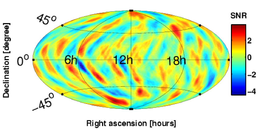
Figure 1: An example map of the signal-to-noise ratio ${\rm SNR}=Y_{\rm opt}/\sigma_{\rm opt}$ for simulated Gaussian noise (see text). The visible structure - fringes with opposite tilt on the northern and southern hemisphere as required by the antipodal symmetry of the antenna lobe - is due to the antenna lobe with which the random background is convolved.

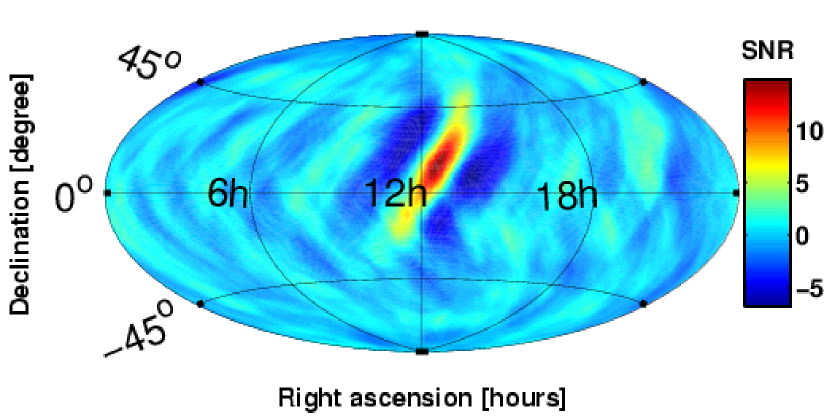
Figure 2: A point source with signal-to-noise ratio (SNR) of 14 was injected at the position of the Virgo galaxy cluster ($\rm 12.5h$, $12.7^{\circ}$). It is nicely recovered. This map also shows the typical structure of the antenna lobe including negative correlation in regions adjoint to the main peak.

For Figure 2 additional coherent noise with a flat power spectrum $H(f)$ and a sidereal time dependent time shift and amplitude modulation appropriate for a true point source was added. The data was produced by splicing together short pieces of data with fixed time shift. The injected source has a signal-to-noise ratio of 14 and is clearly recovered. This figure also shows the typical shape of the radiometer antenna lobe which is given by Eq. 15. In particular it shows that areas adjoint to the main lobe get a negative correlation. This means that a particularly unfortunate set of sources could in principle cancel a lot of the signal.

4 Conclusion

The presented gravitational wave radiometer method aims for optimal detection of localized stochastic gravitational wave sources with a given power spectrum $H(f)$ and significant uptime. It produces a map of point estimates and corresponding variances. The point estimate map corresponds to the true power distribution of gravitational waves $P({\hat{\Omega}})$ convolved with the antenna lobe of the radiometer and an uncertainty determined by the detector noise. This antenna lobe in turn depends on the assumed source power spectrum $H(f)$.

The method is well suited for searching for a stochastic gravitational wave background of astrophysical origin and the LIGO Scientific Collaboration intends to use it on future LIGO science runs starting with S4.

The author gratefully acknowledges his colleagues in the LIGO Scientific Collaboration whose work on building and commissioning ground based gravitational wave detectors as well as computing infrastructure made this research possible. In addition he acknowledges the support of the United States National Science Foundation for the construction and operation of LIGO under Cooperative Agreement PHY-0107417.

References

References

- [1] B. Abbott et al., “Upper Limits on a Stochastic Background of Gravitational Waves,” Phys. Rev. Lett. accepted for publication
- [2] B. Abbott et al., Phys. Rev. D 69, 122004 (2004).
- [3] T. Regimbau, J. A. de Freitas Pacheco Astron. Astrophys. 376, 381 (2001)
- [4] L. Bildsten, Astrophys. J. L89-L93 (1998)
- [5] B. Allen and A.C. Ottewill, Phys. Rev. D 56, 545 (1997)
- [6] N. J. Cornish, Class. Quantum Grav. 18, 4277 (2001)
- [7] B. Allen and J.D. Romano, Phys. Rev. D 59, 102001 (1999).
- [8] N. Christensen, Phys. Rev. D 46, 5250 (1992); É.É. Flanagan, Phys. Rev. D 48, 389 (1993).
- [9] B. Barish and R. Weiss, Phys. Today 52, 44 (1999).
- [10] B. Abbott et al., Nucl. Instrum. Methods A 517/1-3, 154 (2004).