Correlation analysis of stochastic gravitational wave background around 0.1-1Hz

Abstract

We discuss prospects for direct measurement of stochastic gravitational wave background around 0.1-1Hz with future space missions. It is assumed to use correlation analysis technique with the optimal TDI variables for two sets of LISA-type interferometers. The signal to noise for detection of the background and the estimation errors for its basic parameters (amplitude, spectral index) are evaluated for proposed missions.

I introduction

Gravitational wave background generated in the early universe is one of the most fascinating targets in observational cosmology Allen:1996vm ; Maggiore:1999vm . Among others, inflationary theory has a realistic mechanism to generate the background, and indeed confirmation of the background is regarded as another strong support for presence of inflationary phase in the early universe. While we might indirectly detect the inflationary generated background by B-mode polarization analysis of CMB Seljak:1996gy ; Kamionkowski:1996zd , direct detection of the background with gravitational wave detectors is an indispensable approach to study the inflation in more detail. This is because the amplitude of the background is mainly determined by the value of the inflation potential when the gravitational waves cross the Hubble horizon in inflationary epoch. If we can measure the amplitudes at two widely separated frequencies (e.g. $\sim 10^{-17}$Hz and $\sim 0.1$Hz), the global structure of the potential might be constrained Lidsey:1995np ; Turner:1996ck ; bbo (see also Seto:2003kc ). The slope of the spectrum at a given band will also provide us information of the derivative of the potential. Therefore, it is quite meaningful to understand how well we can measure the basic parameters that characterize the spectrum.

Standard slow-roll inflation predicts that the spectrum $\Omega_{GW}(f)$ is nearly flat at frequency regime relevant for the direct detection (Lidsey:1995np ; Turner:1996ck , see Ungarelli:2005qb ; Cooray:2005xr ; Smith:2005mm ; Boyle:2005ug for recent studies). This means that its strain amplitude is expected to be higher at lower frequencies. However, astrophysical foreground would be a fundamental obstacle to directly detect weak inflationary background below $\sim 0.1$Hz. For this reason the band around $\sim 1$Hz is considered to be suitable for the direct detection, and projects such as, the Big Bang Observer (BBO; US) bbo or DECI-hertz interferometer Gravitational wave Observatory (DECIGO; Japan) Seto:2001qf have been proposed (see also Ungarelli:2000jp ; Crowder:2005nr ). For these projects, correlation analysis is a powerful method to observe weak background Michelson(1987) ; Christensen:1992wi ; Flanagan:1993ix ; Allen:1997ad . In this paper prospects of this method are studied quantitatively, from detectability of the background to parameter estimation errors.

This paper is organized as follows; In section II we study basic aspects of the optimal data streams for the Time-Delay-Interferometry (TDI) method, and designed sensitivities of BBO or DECIGO are briefly mentioned. In section III a formal discussion for correlation analysis is presented. We evaluate the expected signal to noise ratio for detecting the background and derive expressions for parameter estimation errors based on the Fisher matrix approach. In section IV numerical results for BBO project are given with using formulas in section III. Section V is a brief summary of this paper.

II TDI variables and their responses to gravitational waves

First we summarize standard notations to discuss stochastic gravitational wave background Allen:1997ad . The plane wave expansion for gravitational waves is given by

$$h_{ab}(t,{\mbox{\boldmath${x}$}})=\sum_{P=+,\times}\int^{\infty}_{-\infty}df\int_{S^{2}}d{\mbox{\boldmath${\Omega}$}}h_{A}(f,{\mbox{\boldmath${\Omega}$}})e^{2\pi if(t-{\mbox{\boldmath${\Omega}$}}\cdot{\mbox{\boldmath${x}$}})}e^{P}_{ab}({\mbox{\boldmath${\Omega}$}}),$$ (1)

where $f$ is the frequency of each mode, ${\Omega}$ is the unit vector for its propagation, $S^{2}$ is a unit sphere for the angular integral $d{\mbox{\boldmath${\Omega}$}}$, and $e^{P}_{ab}$ $(P=+,\times)$ is the basis for the polarization tensor. We assume that the stochastic background is isotropic, unpolarized and static, and express the spectrum of its amplitude $h_{A}(f,{\mbox{\boldmath${\Omega}$}})$ in terms of the logarithmic energy density of the gravitational waves $\Omega_{GW}(f)\equiv 1/\rho_{c}d\rho_{GW}(f)/d\ln f$ ($\rho_{c}$: the critical density) as follows;

$$\left\langle h_{P}^{*}(f,{\mbox{\boldmath${\Omega}$}})h_{P^{\prime}}(f^{\prime},{\mbox{\boldmath${\Omega}$}}^{\prime})\right\rangle=\frac{3H_{0}^{2}}{32\pi^{3}}\delta^{2}({\mbox{\boldmath${\Omega}$}}-{\mbox{\boldmath${\Omega}$}}^{\prime})\delta_{PP^{\prime}}\delta(f-f^{\prime})|f|^{-3}\Omega_{GW}(|f|),$$ (2)

where $H_{0}$ is the Hubble parameter and we fix it at $H_{0}=$70km/sec/Mpc. The symbol $\left\langle...\right\rangle$ represents to take an ensemble average of stochastic quantities.

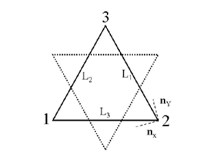
Next we discuss responses of interferometers to incident gravitational waves. We concentrate on a LISA-like detector. Each unit is formed by three spacecrafts at the vertices of a nearly regular triangle, as shown in the solid lines in figure 1 where we also define the labels of its vertices (1,2,3) and arms ($L_{1},L_{2},L_{3}$). We denote the six (one-way) relative frequency fluctuations of the laser light as $y_{ij}(t)$ $(i,j=1,2,3;i\neq j)$. The quantity $y_{ij}(t)$ corresponds to the signal measured at the spacecraft $j$, transmitted from the spacecraft $k(\neq i,\neq j)$ along the arm $L_{i}$. For example, the variable $y_{13}$ responds to a single gravitational wave mode with parameters $(f,{\mbox{\boldmath${\Omega}$}}$ and $e^{P}_{ab})$ as estabrook

$$y_{31}(t)=\frac{1}{2}\frac{{\mbox{\boldmath${n}$}}_{12}\cdot\mbox{\boldmath${e}$}^{P}\cdot{\mbox{\boldmath${n}$}}_{12}}{1-({\mbox{\boldmath${\Omega}$}}\cdot{\mbox{\boldmath${n}$}}_{12})^{2}}(1+{\mbox{\boldmath${\Omega}$}}{\mbox{\boldmath${n}$}}_{12})h_{A}(f,{\mbox{\boldmath${\Omega}$}})(U(t,1)-U(t-\tau,2)),$$ (3)

where ${\mbox{\boldmath${n}$}}_{12}$ is the unit vector from vertex $1$ to vertex $2$, and the function $U(t,i)$ contains information of the phase of the wave at time $t$ and position ${\mbox{\boldmath${x}$}}_{i}$ of vertex $i$. It is given as

$$U(t,j)=\exp\left[-2\pi if(t-{\mbox{\boldmath${\Omega}$}}\cdot{\mbox{\boldmath${x}$}}_{j})\right].$$ (4)

The time delay interferometry (TDI) is an important technique for LISA-type detectors to overcome the laser frequency fluctuations Armstrong et al.(1999) . We follow Ref.Prince:2002hp to summarize the relevant data streams for signal analysis (see also Krolak:2004xp ; Nayak:2002ir ; Corbin:2005ny ). We first define a TDI variable, $\alpha$ as follows;

$$\alpha=y_{21}-y_{31}+y_{13,2}-y_{12,3}+y_{32,12}-y_{23,13},$$ (5)

where we used the notations like $y_{13,2}(t)\equiv y_{13}(t-L_{2})$ and $y_{32,12}(t)\equiv y_{32}(t-L_{1}-L_{2})$. In the same manner we define two other TDI variables $\beta$ and $\gamma$ that are given by cyclic permutations of the subscripts of the variable $\alpha$. These $\alpha$, $\beta$ and $\gamma$ are TDI variables, but their noises are correlated. Thus we define the following new variables $A$, $E$ and $T$ as

$$A = \frac{1}{\sqrt{2}}(\alpha-\gamma),$$ (6)

$$E = \frac{1}{\sqrt{6}}(\alpha-2\beta+\gamma),$$ (7)

$$T = \frac{1}{\sqrt{3}}(\alpha+\beta+\gamma).$$ (8)

As we can easily confirm with using the symmetry of the original data streams $\alpha$, $\beta$ and $\gamma$, the noises of the variables $A$, $E$ and $T$ do not have correlation. In other words, they are orthogonal. We regard them as the fundamental data sets for correlation analysis. Hereafter, we do not discuss differences of the arm lengths $L_{i}$ or their time variations, and simply put $L_{1}=L_{2}=L_{3}=L=const$. Even if the second generation TDI variables Cornish:2003tz ; Shaddock:2003dj are used, our basic results are not changed Krolak:2004xp . As our primary interest is observation of the monopole mode of the background, the motion of the triangle will not be included.

Figure 1: Three vertices $(1,2,3)$ and three arms $(L_{1},L_{2},L_{3})$ of the first unit (solid lines). Configuration of second unit (short-dashed lines) is obtained by $180^{\circ}$ rotation of the first one around its center. Labels for vertices and arms of the second ones are transported with this rotation.

At low frequency regime with $fL\ll 1$, the response of $E$ mode is approximately given as Krolak:2004xp ; white

$$E\simeq\frac{3}{\sqrt{2}}(2\pi fL)^{2}\left[\frac{1}{2}({\mbox{\boldmath${n}$}}_{X}\cdot{\mbox{\boldmath${h}$}}\cdot{\mbox{\boldmath${n}$}}_{X}-{\mbox{\boldmath${n}$}}_{Y}\cdot{\mbox{\boldmath${h}$}}\cdot{\mbox{\boldmath${n}$}}_{Y})\right],$$ (9)

where directions of two unit vectors ${\mbox{\boldmath${n}$}}_{X}$ and ${\mbox{\boldmath${n}$}}_{Y}$ (${\mbox{\boldmath${n}$}}_{X}\perp{\mbox{\boldmath${n}$}}_{Y}$) are given in figure 1. The large parenthesis in eq.(9) is the response of a simple $L$-shaped detector, as often used in the literature of gravitational waves. In the same manner, the $A$ mode asymptotically becomes a simple response obtained by rotating ${\mbox{\boldmath${n}$}}_{X}-{\mbox{\boldmath${n}$}}_{Y}$ system by $45^{\circ}$ on the detector plane Cutler:1997ta . The response of T mode at low frequency regime is $T=O(f^{3})$ in contrast to $A=E=O(f^{2})$ as in eq.(9). This allows us to use the T mode to monitor the detector noise in principle Tinto:2001ii ; Hogan:2001jn .

As for the sources of noises, we take into account the proof mass and optical path noises with parameters $w_{p}$ and $w_{o}$ as

$$S_{y}^{proof-mass}(f) = 2.5\times 10^{-48}w_{p}^{2}(f/1{\rm Hz})^{-2}{\rm Hz^{-1}},$$ (10)

$$S_{y}^{optical-path}(f) = 1.8\times 10^{-37}w_{o}^{2}(f/1{\rm Hz})^{2}{\rm Hz^{-1}}.$$ (11)

The proof mass noise is dominant at low frequency regime. Basic parameters of LISA are $(L,w_{p},w_{o})=(5.0\times 10^{6}{\rm km},1.0,1.0)$ lisa ; Prince:2002hp ; white . For BBO project three possible configurations are discussed bbo , namely BBO-lite: $(2.0\times 10^{4}{\rm km},0.1,4.0\times 10^{-6})$, BBO-standard: $(5.0\times 10^{4}{\rm km},0.01,1.4\times 10^{-6})$ and BBO-grand $(2.0\times 10^{4}{\rm km},0.001,2.6\times 10^{-7})$ bbo . These parameters for BBO configurations were presented in 2003, and we use them for a reference. We should keep in mind that they do not always represent the most up to date designed sensitivities. In the original proposal the second configuration; “BBO-standard” is simply named as “BBO”. In this paper we use the former for the name of a specific configuration and the latter for the name of the project itself. The parameter $w_{0}$ is assumed to scale as $w_{0}\propto\lambda^{3/2}(\epsilon p)^{-1/2}LD^{-2}$ with the laser power $p$ at wavelength $\lambda$, optical efficiency $\epsilon$, the armlength $L$ and the mirror diameter $D$ Larson:1999we . The noises (10) and (11) are defined for the one-way signal $y_{ij}$. For the A, E and T modes the noise spectra are given by Prince:2002hp ; Krolak:2004xp ; white

$$S_{A}(f) = S_{E}(f)=16\sin^{2}(f/2f_{*})\left[3+2\cos(f/f_{*})+\cos(2f/f_{*})\right]S_{y}^{proof-mass}(f)$$ (12)

$$+8\sin^{2}(f/2f_{*})\left[2+\cos(f/f_{*})\right]S_{y}^{optical-path}(f),$$

$$S_{T}(f) = 2\left[1+2\cos(f/f_{*})\right]^{2}\left[4\sin^{2}(f/2f_{*})S_{y}^{proof-mass}(f)+S_{y}^{optical-path}(f)\right]$$ (13)

with $f_{*}\equiv(2\pi L)^{-1}$. We have $f_{*}=0.95$Hz for BBO-standard and $f_{*}=2.4$Hz for BBO-grand and BBO-lite.

As the responses $H_{I}$ ($I=A,E,T$) to the coefficient $h(f,{\mbox{\boldmath${\Omega}$}})$ of each gravitational wave mode are linear, we can express them in a form

$$H_{I}=h_{P}(f,{\mbox{\boldmath${\Omega}$}})R(I,f,{\mbox{\boldmath${\Omega}$}},P).$$ (14)

After taking the average with respect to the direction ${\Omega}$ and polarization $P$ of the incident waves, we obtain the effective noise curve Prince:2002hp ; Larson:1999we ; Cornish:2001qi

$$h_{I}(f)=\left(\frac{\left\langle R^{*}(I,f,{\mbox{\boldmath${\Omega}$}},P)R(I,f,{\mbox{\boldmath${\Omega}$}},P)\right\rangle_{a}}{S_{I}(f)}\right)^{-1/2},$$ (15)

where the symbol $\left\langle...\right\rangle_{a}$ represents the above mentioned average. Due to symmetry of the data streams ($A,E,T$) we have $\left\langle R^{*}(I,f,{\mbox{\boldmath${\Omega}$}},P)R(I,f,{\mbox{\boldmath${\Omega}$}},P)\right\rangle_{a}=0$ for $I\neq J$. This means that the correlation between ($A,E$), ($E,T$) and ($T,A$) vanish for isotropic component of the background. Thus the optimal sensitivity to the isotropic gravitational wave background with all the three variables becomes

$$h_{opt}(f)=\left(\sum_{I=A,E,T}\frac{\left\langle R^{*}(I,f,{\mbox{\boldmath${\Omega}$}},P)R(I,f,{\mbox{\boldmath${\Omega}$}},P)\right\rangle_{a}}{S_{I}(f)}\right)^{-1/2}.$$ (16)

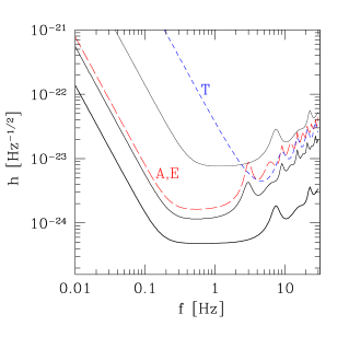
In figure 2 we show some of the results for the three possible BBO configurations (see also Crowder:2005nr ). The $A$ and $E$ modes have the same sensitivity. In the low frequency regime $f\ll f_{*}$ the contribution of the T-mode is negligible to the optimal sensitivity, and we have $h_{opt}(f)\simeq h_{A}(f)/\sqrt{2}$ Prince:2002hp . The currently designed sensitivity of Fabry-Perot type DECIGO is similar to that of BBO-standard kawamura . While the minimum noise floor of DECIGO extends to a higher frequency ($\sim$7.5Hz) than BBO-standard (see figure 2), this difference is not important for observing the inflationary background and we will have similar results for these two cases (in order of magnitude sense). Therefore we do not take up DECIGO separately from BBO-standard.

Figure 2: The optimal sensitivities for BBO-lite (thin solid curve), BBO-standard (solid curve) and BBO-grand (thick solid curve) configurations. The sensitivities for (A,E) modes (long-dashed curve) and T mode (short-dashed curve) are also given for BBO-standard configuration.

III correlation analysis with star-like configurations

Correlation analysis is a powerful approach to detect weak stochastic gravitational wave background Michelson(1987) ; Christensen:1992wi ; Flanagan:1993ix ; Allen:1997ad . If noises of two data streams have no correlation but their responses to gravitational wave background are correlated, we can increase the signal to noise ratio for detection of background by a long term observation. In the case of LISA the orthogonal data streams $A$, $E$ and $T$ do not have correlated responses as mentioned in the last section, and we cannot perform correlation analysis to measure the monopole mode of the background. The situation is different for studying anisotropies of the background, and the correlation between two of the three ($A,E,T$) modes will be useful to extract information of the background generated by Galactic binaries Seto:2004ji ; Kudoh:2004he ; Seto:2004np . For example, we can show that correlation between $A$ and $E$ modes has sensitivity to the hexadecapole mode ($l=4$) under the low frequency approximation. By combining this effect with the time modulation of the signal due to the rotation of the detector, we can get information of low-$l$ moments (e.g. $l=2,4$) of the Galactic gravitational wave background around $\sim 1$mHz that is expected to be highly anisotropic Seto:2004ji ; Kudoh:2004he ; Seto:2004np .

For BBO it is proposed to use another unit for correlation analysis to detect isotropic mode. In figure 1 we show the proposed placement of its two units bbo ; Crowder:2005nr ; Cornish:2001qi . Two units have identical specification. The position of the second unit (dotted lines) is obtained by rotating the first one by $180^{\circ}$ degree with respect to the center of the triangle. We transport the labels of the first one to the second one $(1^{\prime},2^{\prime},3^{\prime},L_{1}^{\prime},L_{2}^{\prime},L_{3}^{\prime})$ with this rotation. For example, the vertex 2’ is at the opposite side of the vertex 2 around the center. The orthogonal TDI variables $A^{\prime},E^{\prime}$ and $T^{\prime}$ of the second unit are defined in the same manner as the first one in the last section.

To discuss the correlated response of two variables $I$ and $J$, we define the overlap reduction function $\gamma_{IJ}(f)$ as Flanagan:1993ix ; Allen:1997ad ; Cornish:2001qi

$$\gamma_{IJ}(f)\equiv 5\left\langle R^{*}_{I}R_{J}\right\rangle_{a}.$$ (17)

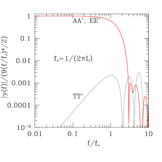
Due to symmetry of the relevant data streams, we have $5\left\langle R^{*}_{I}R_{J}\right\rangle_{a}=5\left\langle R_{I}R^{*}_{J}\right\rangle_{a}$ and the functions $\gamma_{IJ}$ take real numbers. Furthermore, their nonvanishing combinations $\gamma_{IJ}$ $(I\neq J)$ to isotropic mode are only $\gamma_{AA^{\prime}}=\gamma_{EE^{\prime}}$ and $\gamma_{TT^{\prime}}$. Other combinations (e.g. $\gamma_{AE^{\prime}}$, $\gamma_{TA^{\prime}}$) become zero. As in the case of LISA, we can, in principle, study anisotropic components ($l\geq 1$) by correlating two outputs, such as, $(A,E)$ or $(A,E^{\prime})$. However, it would be difficult to observe the cosmological anisotropy of the background around $\sim 1$Hz, considering its expected magnitude $\sim 10^{-5}$ Seto:2004np (see also Kudoh:2005as ). The factor 5 in eq.(17) is the conventional choice Flanagan:1993ix ; Allen:1997ad ; Cornish:2001qi , and we have $\gamma_{IJ}=1$ for two co-aligned detectors at low frequency limit with the simple response function in the large parenthesis of eq.(9). In figure 3 we show these three non-vanishing overlap reduction functions normalized by $9(f/f_{*})^{4}/2$ that comes for the prefactor in eq.(9). These functions are determined purely by the geometry of the placement and scale with the parameter $f_{*}=1/2\pi L$ for any star-like constellation given in figure 1.

Figure 3: The normalized overlap reduction function $\gamma(f)$ for a star-like constellation. These curves have a scaling parameter $f_{*}=c/(2\pi L)$ that is determined by the arm-length.

Now we study correlation analysis in a more detailed manner with Fourier space representation. Each data stream $s_{I}(f)$ is made by gravitational wave signal $H_{I}(f)$ and noise $n_{I}(f)$ as

$$s_{I}(f)=H_{I}(f)+n_{I}(f).$$ (18)

The noise spectrum

$$\left\langle n_{I}^{*}(f)n_{I}(f^{\prime})\right\rangle=\frac{1}{2}\delta(f-f^{\prime})S_{I}(f)$$ (19)

is given in eqs.(12) and (13) for the orthogonal TDI variables $I=\{A,E,T,A^{\prime},E^{\prime},T^{\prime}\}$. We assume that the noises have no correlation (namely $\left\langle n_{I}^{*}n_{J}\right\rangle=0$ for $I\neq J$), and the amplitude of the signal $\left\langle H_{I}(f)^{*}H_{J}(f)\right\rangle$ is much smaller than that of the noise $\left\langle n_{I}(f)^{*}n_{I}(f)\right\rangle$. The latter is the condition where correlation analysis becomes very powerful. We divide the positive Fourier space into frequency segments $F_{i}$ ($i=1,...,N$) with their center frequencies $\{f_{i}\}$ and widths $\{\delta f_{i}\}$. In each segment the width $\delta f_{i}$ is much smaller than $f_{i}$, and the relevant quantities (e.g. $\Omega_{GW}(f)$, $\gamma_{IJ}(f)$) are almost constant. But the width is much larger than the frequency resolution $\Delta f\equiv T_{obs}^{-1}$ ($T_{obs}$: observation period) so that each segment contains Fourier modes as many as $\delta f_{i}/\Delta f\gg 1$.

For correlation analysis we compress the observational data $s_{I}(f)$ by summing up the products $s^{*}_{I}(f)s_{J}(f)$ ($I\neq J$) in each segment $F_{i}$ as

$$\mu_{i}\equiv\sum_{f\in F_{i}}s^{*}_{I}(f)s_{J}(f),$$ (20)

where we omitted the apparent subscript $\{IJ\}$ for the compressed data $\{\mu_{i}\}$ for notational simplicity. As the noises are assumed to be uncorrelated, the statistical mean $\left\langle\mu_{i}\right\rangle$ is arisen by gravitational wave signal. After some calculations with using eqs.(2) (14) and (17) we have a real value

$$\left\langle\mu_{i}\right\rangle=\sum_{f\in F_{i}}\left\langle H_{I}(f)^{*}H_{J}(f)\right\rangle\simeq\frac{3H_{0}^{2}}{20\pi^{2}}f_{i}^{-3}\Omega_{GW}(f_{i})\gamma_{IJ}(f_{i})\frac{\delta f_{i}}{\Delta f}.$$ (21)

The fluctuations around the mean $\left\langle\mu_{i}\right\rangle$ are dominated by the noise under our weak signal approximation, and its variance $\sigma_{i}^{2}$ for the real part of $\mu_{i}$ becomes

$$\sigma_{i}^{2}=S_{I}(f_{i})S_{J}(f_{i})\frac{\delta f_{i}}{8\Delta f}.$$ (22)

As the number of Fourier modes $\delta f_{i}/\Delta f$ in each segment is much larger than unity, the probability distribution function (PDF) for the real part of the measured value $\mu_{i}$ is close to Gaussian distribution due to the central limit theorem as

$$p({\rm Re}[\mu_{i}])\simeq\frac{1}{\sqrt{2\pi\sigma_{i}^{2}}}\exp\left[-\frac{({\rm Re}[\mu_{i}]-\left\langle\mu_{i}\right\rangle)^{2}}{2\sigma_{i}^{2}}\right].$$ (23)

Here we neglected the prior information of the spectrum $\Omega_{GW}(f)$. From eqs.(20) and (21) the signal to noise ratio of each segment becomes

$$SNR^{2}_{i}=\frac{\left\langle\mu_{i}\right\rangle^{2}}{\sigma_{i}^{2}}=\left(\frac{3H_{0}^{2}}{10\pi^{2}}\right)^{2}{T_{obs}}\left[2\delta f_{i}\frac{\gamma_{IJ}(f)^{2}\Omega_{GW}(f)^{2}}{f^{6}S_{I}(f)S_{J}(f)}\right].$$ (24)

Summing up the all the segments quadratically, we get the total signal to noise ratio

$$SNR^{2}=\left(\frac{3H_{0}^{2}}{10\pi^{2}}\right)^{2}T_{obs}\left[2\int_{0}^{\infty}df\frac{\gamma_{IJ}(f)^{2}\Omega_{GW}(f)^{2}}{f^{6}S_{I}(f)S_{J}(f)}\right].$$ (25)

Note that this expression does not depend on the details of the segmentation $\{F_{i}\}$. We can directly obtain the same results by introducing the optimal filter for the product $s_{I}^{*}(f)s_{J}(f)$ to get the highest signal to noise ratio (see e.g. Allen:1997ad ). Eq.(25) is given for a single pair $(I,J)$ of the data streams. As the overlap reduction functions $\gamma_{IJ}$ are “diagonalized” ($\gamma_{IJ}\neq 0$ only for the following combination $(I,J)=(A,A^{\prime}),(E,E^{\prime}),(T,T^{\prime})$ with $I\neq J$), the total signal to noise ratio given by all of these combinations is evaluated by adding their contributions as

$$(SNR)^{2}_{opt}=\left(\frac{3H_{0}^{2}}{10\pi^{2}}\right)^{2}T_{obs}\left[2\sum_{(I,J)}\int_{0}^{\infty}df\frac{\gamma_{IJ}(f)^{2}\Omega_{GW}(f)^{2}}{f^{6}S_{I}(f)S_{J}(f)}\right].$$ (26)

In this paper we mainly study the case with using all these three combinations, unless otherwise stated.

Next we discuss how well we can estimate parameters $\alpha_{m}$ ($m=1,...,M$; $M$: total number of parameters) that characterize the stochastic background spectrum $\Omega_{GW}(f)$. We can apply standard procedure of the maximum likelihood analysis for the compressed data $\{\mu_{i}\}$ with the probability distribution function (23) helstrom . Then the magnitude of the parameter estimation error $\Delta\alpha_{m}$ is evaluated by the Fisher information matrix $\Gamma_{mn}$ that is the inverse of the error covariance matrix $\left\langle\Delta\alpha_{m}\Delta\alpha_{n}\right\rangle$ as

$$\left\langle\Delta\alpha_{m}\Delta\alpha_{n}\right\rangle^{-1}=\Gamma_{mn}=\left(\frac{3H_{0}^{2}}{10\pi^{2}}\right)^{2}T_{obs}\left[2\sum_{(I,J)}\int_{0}^{\infty}df\frac{\gamma_{IJ}(f)^{2}\partial_{\alpha_{m}}\Omega_{GW}(f)\partial_{\alpha_{n}}\Omega_{GW}(f)}{f^{6}S_{I}(f)S_{J}(f)}\right].$$ (27)

The simplest case is the estimation of the amplitude $\Omega_{GW}$ for a flat spectrum $\Omega_{GW}(f)=\Omega_{GW}=const$ in the frequency range relevant for correlation analysis. In this one parameter estimation with $\alpha_{1}=\ln\Omega_{GW}$, the expected error becomes

$$\Delta\alpha_{1}=\frac{\Delta\Omega_{GW}}{\Omega_{GW}}=(SNR)^{-1}.$$ (28)

We can easily confirm this by using eqs.(26) and (27). Actually, the above result (28) holds for the case when we estimate only the overall amplitude of the spectrum $\Omega_{GW}(f)$ with a known frequency dependence.

A more realistic situation is to estimate two parameters, the amplitude $\alpha_{1}=\ln\Omega_{GW,F}$ and the slope $\alpha_{2}=n$, assuming that the spectrum has a power-law form

$$\Omega_{GW}(f)=\Omega_{GW,F}(f/F)^{n}$$ (29)

around a central frequency $F$. In this case we do not have the simple result (28) for the first parameter $\alpha_{1}=\ln\Omega_{GW,F}$, as the two parameters have correlation. The magnitude of the error $\Delta\alpha_{2}$ for the slope does not depend on the choice of the frequency $F$, as we can understand from its geometrical meaning. We can also confirm this directly with using eq.(27). In contrast, the error $\alpha_{1}$ and the correlation coefficient $r\equiv{\left\langle\Delta\alpha_{1}\alpha_{2}\right\rangle}/({\left\langle\Delta\alpha_{1}^{2}\right\rangle\left\langle\Delta\alpha_{2}^{2}\right\rangle})^{1/2}$ depend on the frequency $F$. With a suitable choice of $F$ we can diagonalized the covariance matrix $\left\langle\Delta\alpha_{i}\alpha_{j}\right\rangle$ $(i=1,2)$. Once we get the errors $\Delta\alpha_{i}$ or signal to noise ratio for a specific combination $(\Omega_{GW,F},n)$, we can easily obtain the results for a different amplitude $\Omega_{GW,F}$ (but the same slope $n$) with using scaling relations as

$$SNR\propto\Omega_{GW,F},~{}~{}~{}\Delta\alpha_{i}\propto\Omega_{GW,F}^{-1},~{}~{}~{}r\propto\Omega_{GW,F}^{0}.$$ (30)

It is straightforward to confirm these relations with eqs.(26) and (27).

So far we have assumed the situation (weak-signal approximation) that the detector noise $\{n_{I}(f)\}$ is much larger than the gravitational wave background $\{H_{I}(f)\}$. When the latter becomes comparable to the former, the background $H_{I}(f)$ itself becomes a significant source of the fluctuations for measuring $\left\langle\mu_{i}\right\rangle$ in eq.(21) Allen:1997ad ; Kudoh:2005as . For the strong signal limit, the signal to noise ratio becomes a asymptotic value of order $SNR\sim(T_{obs}f)^{1/2}$ that is $10^{3}\sim 10^{4}$ for BBO band with a reasonable observational time. In a recent paper Kudoh:2005as it is shown that for BBO band ($\gtrsim 0.1$Hz) the weak signal approximation provides a fairly good estimation for SNR smaller than $\sim 200$. On the other hand, the performance of the Fisher matrix approach becomes worse at low SNR. Therefore, our expressions in this section are expected to be reasonable for the background observed with $10\lesssim SNR\lesssim 200$.

IV Numerical results for BBO

In this section we present numerical results for BBO project. Its primary goal is direct detection of the stochastic gravitational wave background generated at inflation. As the standard slow-roll inflation predicts a nearly flat spectrum at BBO band, we first assume that the true spectrum has a simple form: $\Omega_{GW}(f)=\Omega_{GW}=const$. By evaluating eq.(26) numerically, we obtain the signal to noise ratio for three possible BBO configurations as

$$SNR = 1.03\left(\frac{\Omega_{GW}}{10^{-15}}\right)\left(\frac{T_{obs}}{10{\rm yr}}\right)^{1/2}~{}~{}~{}({\rm BBO-lite}),$$ (31)

$$SNR = 25.1\left(\frac{\Omega_{GW}}{10^{-16}}\right)\left(\frac{T_{obs}}{10{\rm yr}}\right)^{1/2}~{}~{}~{}({\rm BBO-standard}),$$ (32)

$$SNR = 251.2\left(\frac{\Omega_{GW}}{10^{-16}}\right)\left(\frac{T_{obs}}{10{\rm yr}}\right)^{1/2}~{}~{}~{}({\rm BBO-grand}).$$ (33)

The magnitude $\Omega_{GW}=10^{-15}$ is close to the upper limit of the amplitude around the BBO band that is consistent with the current CMB observation Turner:1996ck . While specification of BBO-lite is not enough to detect the level $\Omega_{GW}\sim 10^{-15}$ with a sufficient signal to noise ratio, BBO-grand has potential to detect the background close to $\Omega_{GW}\sim 10^{-18}$.

To calculate the above results we simply integrated eq.(26) from $f=0$ to $f=\infty$. This would be too optimistic considering the fact that the frequency below $f\lesssim 0.2$Hz might be significantly contaminated by cosmological white dwarf binaries Farmer:2003pa . Above $\sim 0.2$Hz we still have to clean the foreground produced by the binaries made by neutron stars or black holes Seto:2001qf ; Ungarelli:2000jp . While it is not clear how well we can actually perform this cleaning (see Cutler:2005qq for recent study), we calculate a less optimistic prediction than eqs.(31)(32) and (33) by introducing a lower frequency cut-off $f_{cut}$ at $f_{cut}=0.2$Hz for the integral (26). Then the above relations become

$$SNR = 0.98\left(\frac{\Omega_{GW}}{10^{-15}}\right)\left(\frac{T_{obs}}{10{\rm yr}}\right)^{1/2}~{}~{}~{}({\rm BBO-lite}),$$ (34)

$$SNR = 17.3\left(\frac{\Omega_{GW}}{10^{-16}}\right)\left(\frac{T_{obs}}{10{\rm yr}}\right)^{1/2}~{}~{}~{}({\rm BBO-standard}),$$ (35)

$$SNR = 116.0\left(\frac{\Omega_{GW}}{10^{-16}}\right)\left(\frac{T_{obs}}{10{\rm yr}}\right)^{1/2}~{}~{}~{}({\rm BBO-grand}).$$ (36)

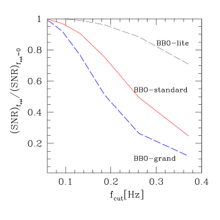
In figure 4 we show how the signal to noise ratio changes with this cut-off frequency. BBO-lite is less sensitive to $f_{cut}$, compared with other two configurations. This is because its minimum of the noise curve is at higher frequency than BBO-standard or BBO-grand, as in figure 2. The upper cut-off frequency is not important for our results, if it is higher than $\sim 1$Hz. Therefore we do not discuss its effects. From figure 2 we can expect that the contribution of T-mode to the total SNR is small. Actually, even if we remove ($T,T^{\prime}$) correlation from eq.(26), the prefactors in eqs.(34)(35) and (33) change less than 1%. We also study the case with completely aligned two units on a single triangle for correlation analysis. The total SNR is obtained by putting $\gamma_{IJ}=5\delta_{IJ}$ and $S_{I}(f)=h_{I}(f)^{2}$ in eq.(26). Here $h_{I}(f)$ is the effective noise curve for $I$-mode given in figure 2. We find that the above prefactors become 0.98, 17.4 and 116.1 respectively, and are very close to the results with the proper transfer functions. Therefore, we can approximately discuss performance of a star-like constellation in a very convenient manner with the effective noise curves that are often used to represent specification of an interfereometer.

Figure 4: Dependence of the signal to noise ratio on the lower cut-off frequency $f_{cut}$.

Figure 5: Error ellipses ($2\sigma$; 86%CL) for two dimensional parameter estimation with different lower cut-off frequencies $f_{cut}$ (dashed curve: $f_{cut}=0$, solid curve: $f_{cut}=0.2$Hz, the dotted curve: $f_{cut}=0.3$Hz). The fisher matrix approach is used. The central frequency $F$ is set at $F=1$Hz that is slightly higher than the optimal sensitivity for measuring the background with above two BBO configurations. The true values of the spectrum $\Omega_{GW}(f)$ are $\Omega_{GW,F}=10^{-16}$ and $n=0$.

Figure 6: Same as figure 5, but with the central frequencies $F$ at $0.26$Hz (BBO-standard) and $0.25$Hz (BBO-grand). The two dimensional covariance matrices are diagonalized with $f_{cut}=0.2$Hz.

Now we move to the case with estimating two parameters $(\alpha_{1},\alpha_{2})=(\ln\Omega_{GW,F},n)$ for the assumed spectrum shape $\Omega_{GW}(f)=\Omega_{GW,F}(f/F)^{n}$. We fix the true values of the parameters at $n=0$ and $\Omega_{GW,F}=10^{-16}$, and set the lower cut-off frequency $f_{cut}$ at 0.2Hz. As we discussed in the last section, the estimation error for the slope $n$ does not depend on the choice of the central frequency $F$, and we get

$$\left\langle\Delta\alpha_{2}^{2}\right\rangle^{1/2}\simeq\Delta n\simeq 0.23~{}~{}~{}(0.039),$$ (37)

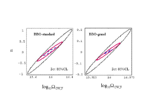
for BBO-standard (BBO-grand, respectively). In contrast, the error $\Delta\alpha_{1}$ for the amplitude $\Omega_{GW,F}$ and the correlation coefficient $r$ depend on the frequency $F$. From observed data we can determine the profile of the spectrum $\Omega_{GW}(f)$ relatively well around the optimal frequency region where the signal to noise ratio accumulates in eq.(26). However, if we take the central frequency $F$ away from this optimal region, the estimated amplitude $\Omega_{GW,F}$ at the frequency $F$ would be strongly affected by the error of the slope $n$. Consequently, the correlation between errors of the two parameters $(\ln\Omega_{GW,F},n)$ becomes strong. In figure 5 we show $2\sigma$-contour map expected for the two parameter fitting. In this figure we take $F=1$Hz that is higher than the optimal frequency region around $0.2\sim 0.4$Hz (see figure 4). We can observe a strong correlation between two fitting parameters, and we have $|r|>0.96$ for the results given in figure 5.

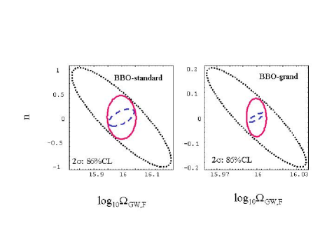
We searched the central frequency $F$ that makes the correlation coefficient $r=0$, and found $F=0.26$Hz (BBO-standard) and 0.25Hz (BBO-grand) for the lower cut-off frequency at 0.2Hz. With these choices for the frequency $F$, the error $\Delta\alpha_{1}$ for the amplitude are given by $SNR^{-1}$ as eq.(28), as the two dimensional variance matrix $\left\langle\Delta\alpha_{i}\Delta\alpha_{j}\right\rangle$ is now diagonalized. In figure 6 we plot the error ellipses with these frequencies $F$. Compared with figure 5, the error for the amplitude $\Omega_{GW,F}$ becomes significantly smaller. We can also understand the direction of the ellipse (or the sign of the coefficient $r$) with an argument similar to the discussion given just after eq.(37).

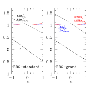
So far we have studied the results mainly for a specific model $\Omega_{GW}(f)=10^{-16}$ at the BBO band. Here we analyze how various quantities depend on the spectral index $n$ for the two dimensional parameter fitting ($\alpha_{1}=\ln\Omega_{GW,F}$, $\alpha_{2}=n$) with assumed spectral form $\Omega_{GW}=\Omega_{GW,F}(f/F)^{n}$. We fix $\Omega_{GW,F}=10^{-16}$, $f_{cut}=0.2$Hz, $F=0.26$ for BBO-standard, 0.25Hz for BBO-grand, but change the slope $n$. Then the signal to noise ratio, the magnitude of errors $(\Delta\alpha_{1},\Delta\alpha_{2})$, and their correlation coefficient $r$ between them are evaluated as functions of the slope $n$. The results are presented in figure 7. Note that the signal to noise ratio and the error for the amplitude $\Omega_{GW,F}$ depend very weakly on the slope. This is because the central frequency $F$ is in the optimal frequency region. With this figure and the numerical results given so far, we can get relevant quantities for various combinations $(\Omega_{GW,F},n)$ by using the scaling relations given in eq.(30).

Figure 7: Dependence of various quantities to the slope $n$. SNR (solid curve) and two errors $\Delta\alpha_{1}$ (dotted curve) and $\Delta\alpha_{2}$ (short-dashed curve) are normalized by their values at $n=0$. The long-dashed curve represent the correlation coefficient $r$. The central frequencies are $F=0.26$Hz (BBO-standard) and $F=0.25$Hz (BBO-grand).

V summary

In this paper we studied prospects for the direct measurement of the stochastic gravitational wave background by correlation analysis. As a concrete example, we explicitly examined the case with possible BBO configurations that use two sets of three spacecrafts to form a star-like constellation. We calculated not only the signal to noise ratio for detection, but also how accurately we can measure the basic parameters that characterize the spectrum $\Omega_{GW}(f)$, such as its amplitude $\Omega_{GW,F}$ or its slope $n$.

While it is difficult to detect a level $\Omega_{GW}\sim 10^{-15}$ with BBO-lite, BBO-grand has potential to detect the background close to $\Omega_{GW}\sim 10^{-18}$ in 10 years. When we try to measure the amplitude and the slope simultaneously for the spectral shape $\Omega_{GW}(f)=\Omega_{GW,F}(f/F)^{n}$, their errors can be highly correlated and the estimation of the amplitude might be degraded, compared with the single parameter fitting for a flat spectrum $\Omega_{GW}(f)=\Omega_{GW}$. If we take the central frequency $F$ around the optimal sensitivity for the correlation analysis, we can nearly diagonalized the two dimensional error covariance matrix.

While we showed the impacts of the low frequency cut-off associated with the potential astrophysical foreground that might be difficult to subtract from the data streams, it is not clear how well we can clean the foreground made by black hole or neutron star binaries above $\sim 0.2$Hz. These aspects, especially in relation to the correlation analysis, must be clarified to properly understand prospects for the measurement of weak stochastic background (e.g. form inflation). In addition we have assumed that the detector noises between combinations $(A,A^{\prime})$, $(E,E^{\prime})$ and $(T,T^{\prime})$ are uncorrelated. In reality they must have correlations to some degree, and estimation of their magnitude is crucial for discussing the sensitivity accessible by correlation analysis Flanagan:1993ix ; Allen:1997ad .