Recollapsing Bianchi I brane worlds

Abstract

We investigate the possibility for a flat Bianchi I brene Universe to recollaps due to the presence of a negative ”dark radiation” and an anisotropic stress in the form of homogeneous magnetic field, localized on the brane.

Sternberg Astronomical Institute, Universitetsky prospekt, 13, Moscow 119899, Russia

^‡ Electronic mail: tpv@xray.sai.msu.ru
^† Electronic mail: lesha@sai.msu.ru

The cosmology of a brane Universe, intensively studied during last several years, has a variety of possible regimes. Some of these are impossible in the standard cosmological scenario. The quadratic stress-energy term in the right-hand side of the effective equation of motion [1, 2] can result in a nonstandard effective equation of state of a brane matter $p=(\gamma-1)\mu$ with $2<\gamma\leq 4$, which is forbidden in the standard cosmology. Another important feature of brane models is the presence of projection of 5-dimensional Weil tensor onto the brane in the equations of motion. This projection can be decomposed into scalar, vector and tensor parts [3]. The scalar part, the only compatible with FRW metric on a brane, also called ”dark radiation”. It can be either positive or negative, violating in the latter case the positive energy condition. Both these features (the quadratic corrections and the presence of the ”dark radiation”) can significantly modify the cosmological dynamics even in the simplest case of an FRW brane. One of the most important modifications alters future asymptotic, because a large enough negative ”dark radiation” can cause a recollaps of a flat brane Universe [4].

The dynamics of a Bianchi I brane also have been studied in detail. In general, as we lift the assumption of spatial isotropy, possible sources of an anisotropic stress should be taken into account. However, the tensor part of the Weil tensor projection onto a brane, being a nonlocal anisotropic stress, has no evolution equation [3]. When some form of nonlocal anysotropic stress is put into equation of motion ”by hand”, the resulting dynamics significantly depends on the ansatz chosen[6, 7]. On the other hand, in the absence of the Weil tensor, a Bianchi I brane with a perfect fluid allows a complete description [8, 9].

The next step in understanding details of brane cosmology have been done in [5], when a Bianchi I brane with a homogeneous magnetic field is studied. Being a source of anisotropic stress, the magnetic field is localized on the brane. The nonlocal anisotropic stress was chosen to be zero (so that the equations of motion can be written in a closed form), the ”dark energy” ${\cal U}$, however, can not vanish identically, because the magnetic field enters as a source term into the evolution equation for ${\cal U}$ (see below). The resulting dynamical system has many stable points and a very complex behavior. Due to this complexity some important issues of magnetic brane evolution remain unclear even after a careful stable point analysis of [5] and require numerical studies.

Denoting the combination of the gravitational constant $G$ and the brane tension $\lambda$ as a new parameter $\chi=(8\pi G\lambda)^{-1}$, one can write the set of equations which governs the evolution of a brane magnetic Universe in the form (see a detailed derivation and a description of the reference frame used in [5])

$$\Theta^{2}=3\rho+\frac{3}{2}\sigma^{2}+\frac{3}{2}h^{2}+\chi(\frac{3}{2}\rho^{2}+\frac{3}{2}\rho h-\frac{3}{4}h^{4})+18\chi{\cal U}$$ (1)

$$\dot{h}=-\frac{2}{3}\Theta h-2\sigma_{+}h$$ (2)

$$\dot{\rho}=-\gamma\Theta\rho$$ (3)

$$\dot{\Theta}=-\frac{1}{3}\Theta^{2}-\sigma^{2}+\frac{1}{2}[(3\gamma-2)\rho+h^{2}]-\frac{\chi}{8}[4(3\gamma-1)\rho^{2}+(6\gamma+4)\rho h^{2}+3h^{4}]-6\chi{\cal U}$$ (4)

$$\dot{\cal U}=-\frac{4}{3}\Theta{\cal U}-\frac{h^{2}}{6}[\theta h^{2}+\frac{5}{3}\sigma_{+}h^{2}-3\gamma\sigma_{+}\rho]$$ (5)

$$\dot{\sigma}_{+}=-\Theta\sigma_{+}-\sigma^{2}_{12}-\sigma^{2}_{13}+\frac{1}{3}h^{2}(1-\frac{\chi}{2}[(3\gamma-2)\rho+\frac{4}{3}h^{2}])$$ (6)

$$\dot{\sigma}_{-}=-\Theta\sigma_{-}-\frac{1}{\sqrt{3}}(\sigma^{2}_{12}-\sigma^{2}_{13})$$ (7)

$$\dot{\sigma}_{23}=-\Theta\sigma_{23}-2\sigma_{12}\sigma_{13}$$ (8)

$$\dot{\sigma}_{12}=-\Theta\sigma_{12}+(3\sigma_{+}+\sqrt{3}\sigma_{-})\sigma_{12}+\sigma_{13}\sigma_{23}$$ (9)

$$\dot{\sigma}_{13}=-\Theta\sigma_{13}+(3\sigma_{+}-\sqrt{3}\sigma_{-})\sigma_{13}+\sigma_{12}\sigma_{23}$$ (10)

Here $\Theta=3H$ is the volume expansion rate, $h$ is the nonvanishing component of the magnetic field (we use the reference frame in which two other components of the magnetic vector vanish), $\sigma_{\mu\nu}$ is the shear tensor. The variables $\sigma_{+}$ and $\sigma_{-}$ are connected with the shear components as follows

$$(\sigma_{11},\sigma_{22},\sigma_{33})=(-2\sigma_{+},\sigma_{+}+\sqrt{3}\sigma_{-},\sigma_{+}-\sqrt{3}\sigma_{-}).$$

Moreover, it is possible to define new shear variables $\sigma_{A}$, $\sigma_{B}$, $\sigma_{C}$ using the transformation

$$\sigma_{12}+i\sigma_{13}=\sigma_{A}e^{i\varphi}$$ (11)

$$\sqrt{3}\sigma_{-}+i\sigma_{23}=(\sigma_{B}+i\sigma_{C})e^{2i\varphi}$$ (12)

Due to symmetries of our dynamical system, the equation of motion for the phase $\varphi$ has the form

$$\dot{\varphi}=\sigma_{C}$$

and the phase decouples from the system. The shear part of the dynamical system takes the form [5]

$$\dot{\sigma}_{+}=-\Theta\sigma_{+}-\sigma_{A}+\frac{1}{3}h^{2}(1-\frac{\chi}{2}[(3\gamma-2)\rho+\frac{4}{3}h^{2}])$$ (13)

$$\dot{\sigma}_{A}=(-\Theta+3\sigma_{+}+\sigma_{B})\sigma_{A}$$ (14)

$$\dot{\sigma}_{B}=-\Theta\sigma_{B}-\sigma^{2}_{A}+2\sigma^{2}_{C}$$ (15)

$$\dot{\sigma}_{C}=(-\Theta-2\sigma_{B})\sigma_{C}$$ (16)

Before describing our numerical results for the general system (1)-(5), (13)-(16) we summarize the conditions for recollaps in simpler models.

If the matter content of the brane Universe is a perfect fluid only (so that $h=0$) , the future recollaps conditions can be found analytically. First of all, we can see from eq.(5) that ${\cal U}$ in this case behaves as radiation, ${\cal U}={\cal U}_{0}/a^{4}$, where $a$ is a mean scale factor. The sign of ${\cal U}$ remains unchanged during the cosmological evolution.

For an isotropic Universe the recollaps conditions have a very simple form. Indeed, for $\gamma>4/3$ the ${\cal U}$ - term in eq.(1) falls less rapidly than the matter terms making the future recollaps inevitable for any initial negative ${\cal U}$.

For $\gamma=4/3$ the first and the last terms in the r.h.s. of (1) are equally important in a low-energy regime, and the condition for collapse is $\rho<-6\chi{\cal U}$. For $2/3<\gamma<4/3$ all three nonzero terms in r.h.s. of (1) are important. Consider, for example, the case of $\gamma=1$. For the dust-like matter $\rho=\rho_{0}/a^{3}$, and assuming that $\rho_{0}$, ${\cal U}_{0}$ are initial values of matter and ”dark radiation” densities, taken when $a_{0}=1$, we can substitut the scale factor dependences of $\rho$, $\rho^{2}$ and ${\cal U}$ into (1). As a result, we obtain that the condition $H=0$ leads to a cubic equation for the scale factor

$$a^{3}+6\chi\frac{{\cal U}_{0}}{\rho_{0}}a^{2}+\frac{\chi\rho_{0}}{2}=0.$$

This equation has positive roots only for $\rho_{0}^{4}<-64\chi^{2}{\cal U}_{0}^{3}$. A root which is bigger than $1$ corresponds to the future of the Universe under consideration and indicates the point of recollaps. A root with $a<1$ describes the past and corresponds to a bounce.

A similar treatment can be performed for any other $\gamma>2/3$. If $\gamma<2/3$, even the quadratic stress-energy correction term, proportional to $\rho^{2}$ falls less rapidly than ${\cal U}$, and the recollaps in the future becomes impossible.

If we add a geometrical anisotropy without an anisotropic stress, the situation does not change significantly. Indeed, the shear scalar $\Sigma=3\sigma_{+}^{2}+\sigma_{A}^{2}+\sigma_{B}^{2}+\sigma_{C}^{2}$ behaves as $\Sigma=\Sigma_{0}/a^{6}$, and we only have an additional term in the equation $H(a)=0$. For example, the system with cosmological constant $\Lambda$ (which corresponds to $\gamma=0$) and shear gives

$$\Sigma_{0}/a^{6}+\Lambda+(\chi/2)\Lambda^{2}+6\chi{\cal U}_{0}/a^{4}=0$$

This gives us the condition for $H=0$ to be possible as $\Lambda^{2}(1+(\chi/2)\Lambda)^{2}<-32\Sigma_{0}\chi^{3}{\cal U}_{0}^{3}$.

In a similar way we can treat other values of $\gamma$. As the shear $\Sigma$ falls more rapidly than the dark radiation ${\cal U}$, it becomes negligible in the low-energy limit, and for $\gamma>4/3$ with ${\cal U}<0$ a recollaps remains inevitable. The condition for $\gamma=4/3$ also remaines unchanged.

If we introduce an anisotropic stress, the shear and ”dark radiation” can no longer be expressed in a simple form as a function of the scale factor due to source terms in eqs.(5)-(6). In particular, now ${\cal U}$ does not proportional to $a^{-4}$ and attribution of the name ”dark radiation” to ${\cal U}$ becomes nothing but tradition. The problem of possible future recollaps of a brane Universe with a homogeneous magnetic field should be therefore investigated numerically. Our main goal in this paper is to describe qualitatively the influence of the magnetic field on the possibility of recollaps, keeping in mind that the non-compactness of our phase space makes it impossible to introduce of a simple reasonable measure on it.

Two main features distinguish the magnetic case from the case without anisotropic stress.

• The $h^{4}$-term in (1) has minus sign, so the recollaps can occur even with nonnegative dark energy ${\cal U}$ if magnetic field $h$ is large enough.

• The sigh of dark energy ${\cal U}$ can change during the cosmological evolution.

The sign change of ${\cal U}$ from positive to negative can lead to a recollaps for positive initial ${\cal U}$ even when $h$ is not large (of course, in this case ${\cal U}<0$ at the maximal expansion point). The opposite change from negative to positive values could in principal enlarge zones in initial condition space which do not lead to collapse. Both these possibilities are allowed by the equations of motion.

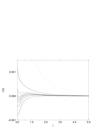
Figure 1: Some trajectories which allow a transition from negative to positive values of ”dark energy”

However, in our numerical studies we have mostly noticed the transition from plus to minus for the sign of ${\cal U}$. Some transitions minus $\to$ plus were constructed using specially adjusted initial conditions, all of them appeared to be part of a zigzag-like behavior and are not important for a general picture (see Fig.1). On the contrary, plus $\to$ minus transitions are in some sense typical. As a result, in all our simulations zones of initial conditions, escaping a recollaps shrink in comparison with similar models without a magnetic field.

Some numerical results are shown in Fig. 2 for $\gamma=4/3$ using $(H,\mu)$ slices of initial condition space. In all plots we put $\chi=1$. White zones represent the initial conditions leading to eternal expansion, gray zones lead to recollaps, while initial conditions from black zones are forbidden by the constraint (1). We can see that the zones, leading to recollaps enlarge and begin to contain some part of ${\cal U}>0$ initial conditions as compared to $H=0$. However, there is still a part of initial state space providing an eternal expansion.

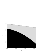
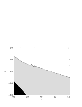
Figure 2: The future fate of a brane magnetic Universe, starting the evolution from $\sigma_{A}=1.3$, $\sigma_{B}=\sigma_{C}=1.1$. Initial $h=0$(left) and $h=2$ (right). White zone corresponds to eternal expansion, gray zone - to recollaps, black zone represent initial condition, forbidden by the constraint equation (1). In this plot $\gamma=4/3$

Similar plots for $\gamma=1$ are shown in Fig.3.

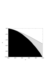
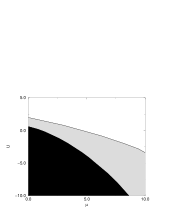
Figure 3: The same as in Fig.2, but for $\gamma=1$

Different plots, using the $(h,\mu)$ slices of the initial condition space with the initial ${\cal U}$ fixed are represented in Fig.4. In particular, we can see how a recollaps being impossible for initial ${\cal U}\geq 0$ without a magnetic field becomes possible for nonzero $h$.

As a result, we can see that a homogenios magnetic field, localized on a brane diminishes the set of initial conditions, which results in a big Universe, resembling our oun. The set of initial conditions, leading to a recollaps, increases. However, this change is not drastic, and we can always find reasonable initial data for an eternally expanding Universe even if initial magnetic field is large.

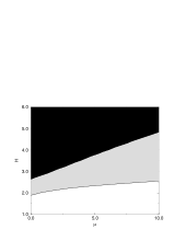
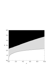
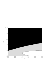
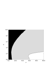
Figure 4: The future fate of a brane magnetic Universe, represented in $(h,\mu)$ slices of the initial condition space. Initial shear values are the same as in Fig.2. Initial values of ” dark energy” are (from left to the right) ${\cal U}=1$, ${\cal U}=0$, ${\cal U}=-1$ and ${\cal U}=-10$. The equation of state parameter $\gamma=4/3$.

References

- [1] Binetruy P, Deffayet C, and Langlois D, Nucl. Phys. B 565, 269 (2000).
- [2] Cline J M, Grojean C and Servant G, Phys. Rev. Lett. 83, 4245 (1999).
- [3] Maartens R, Phys. Rev. D 62, 084023 (2000).
- [4] Santos M G, Vernizzi F and Ferreira P G, Phys. Rev. D 64 063506.
- [5] Barrow J, Hervik S, Class.Quant.Grav. 19, 155 (2002).
- [6] Campos A, Maartens R, Matravers D and Sopuerta C F, Phys. Rev. D 68 103520 (2003).
- [7] A.Fabbri, D.Longlois, D.A.Steer and R.Zegers, JHEP 0409 (2004) 025.
- [8] Campos A, Sopuerta C F, Phys. Rev. D 63 104012 (2001).
- [9] Campos A, Sopuerta C F, Phys. Rev. D 64 104011 (2001).