Cosmological particle production and the precision of the WKB approximation

Abstract

Particle production by slow-changing gravitational fields is usually described using quantum field theory in curved spacetime. Calculations require a definition of the vacuum state, which can be given using the adiabatic (WKB) approximation. I investigate the best attainable precision of the resulting approximate definition of the particle number. The standard WKB ansatz yields a divergent asymptotic series in the adiabatic parameter. I derive a novel formula for the optimal number of terms in that series and demonstrate that the error of the optimally truncated WKB series is exponentially small. This precision is still insufficient to describe particle production from vacuum, which is typically also exponentially small. An adequately precise approximation can be found by improving the WKB ansatz through perturbation theory. I show quantitatively that the fundamentally unavoidable imprecision in the definition of particle number in a time-dependent background is equal to the particle production expected to occur during that epoch. The results are illustrated by analytic and numerical examples.

I Introduction

Particle production by gravity in a slowly expanding universe can be described using quantum field theory in curved spacetime (QFTCS) DeWitt75 ; BirDav82 ; Ful89 ; GriMamMos94 ; For97 ; Jac03 ; MukWin05 . A well-known feature of QFTCS is the absence of an absolute definition of vacuum and particles for quantum fields in arbitrary curved backgrounds (see e.g. Dav84 ). The number of particles detected by an observer depends on the observer’s motion, and there are no preferred observers in a general spacetime. If the universe is sufficiently spatially flat and expands sufficiently slowly so that the four-curvature scale is much larger than the wavelength of a field mode, there is a natural (if approximate) definition of the vacuum state for that mode: the adiabatic vacuum with respect to a given fiducial time $t_{0}$. This is the vacuum state seen by “approximately inertial” observers at $t=t_{0}$. However, an adiabatic vacuum state defined at $t=t_{0}$ is generally an excited state with respect to the vacuum defined at another time $t_{1}\neq t_{0}$. Such field excitations are interpreted as particles produced by gravity. Since there is no single physically preferred vacuum state, we speak of an apparent particle production. The “real” particle content of a given quantum state of the field cannot be unambiguously established without referring to a particular physical experiment where the vacuum state is observed or prepared.

For instance, the most straightforward definition of the vacuum state (the “instantaneous diagonalization” of the Hamiltonian) yields an infinite apparent particle production in some generic cases Ful79 , while the adiabatic vacuum exhibits finite particle densities in the same cases. It has been also proposed Par69 that the vacuum state should be chosen to minimize the apparent particle number observed at a time $t_{0}$. This prescription is physically reasonable and yields a quantum state close to an adiabatic vacuum, but the resulting state will in general depend on the choice of $t_{0}$. A natural and unambiguous definition of the vacuum state is available only in regimes where gravity becomes negligible. So the concept of particles can be used in curved spacetimes only in an approximate sense which becomes more precise in slow-changing, almost flat geometries, and also for high-energy particles. The central theme of this paper is to explicitly analyze the precision of this approximation.

The prescription of the adiabatic vacuum is based on the WKB approximation and has been particularly useful in the context of QFTCS (see e.g. Par69 ; ZelSta71 ; BunChrFul78 ). It is well known that the WKB approximation is applicable to equations such as

$$\frac{d^{2}x}{dt^{2}}+\omega^{2}(t)x=0,$$ (1)

where $\omega(t)>0$ is a time-dependent frequency function. The approximate solutions can be found in the form of an asymptotic series in the adiabatic parameter $T^{-1}$, where $T$ is the characteristic variation timescale of the function $\omega(t)$, which is assumed to be slow-changing BenOrs78 . Using the $n$-th order WKB approximation, one can define adiabatic vacuum states of order $n$ BunChrFul78 . The difference between $n$-th order adiabatic vacua defined at different fiducial times is characterized by apparent particle occupation numbers, which are of order $T^{-1-n}$; this is then the imprecision in the resulting definition of particle numbers. A brief overview of the calculation of cosmological particle production using the adiabatic vacuum prescription is given in Sec. II.2.

It is known that the WKB approximation involves a divergent asymptotic series and thus cannot be used beyond a certain order $n_{\max}$. Therefore, particle occupation numbers computed with respect to an adiabatic vacuum are defined only with a certain fundamentally limited accuracy. If one uses the adiabatic vacuum of the optimal order $n_{\max}$, one obtains particle occupation numbers up to an uncertainty of order $T^{-1-n_{\max}}$, and this accuracy cannot be improved any further.

Since typical particle numbers produced in vacuum by smooth geometries are exponentially small BirDav82 , namely of order $\exp(-\omega T)$, it is a priori unclear whether even the best attainable precision $\sim T^{-1-n_{\max}}$ is adequate for the description of particle production. The exponentially small particle numbers can be calculated if one applies perturbation theory techniques to the WKB ansatz; various such techniques are outlined in Sec. III. I shall summarily refer to these techniques as the perturbatively improved WKB.

Although the WKB expansion, being a power series in $T^{-1}$, necessarily misses any exponentially small terms, the quantity $T^{-n_{\max}}$ can be of order $\exp(-\omega T)$ if $n_{\max}$ is sufficiently large, say of order $T$. The main result of the present work is an explicit estimate of the optimal order $n_{\max}$ and of the resulting optimal precision of the WKB series. The current literature does not appear to offer such direct estimates. It is difficult to analyze the WKB series since there is no closed-form expression for the $n$-th term of that series. To circumvent this difficulty, I use a particular perturbatively improved WKB technique—the so-called Bremmer series (see Sec. III.2). I show in Sec. IV that $n_{\max}=O(\omega T)$ and the error of the optimally truncated series is exponentially small. More precisely, for Eq. (1) with analytic functions $\omega(t)$, the optimal order $n_{\max}$ of the WKB approximation at $t=t_{0}$ is found as

$$n_{\max}=\min_{t_{i}}\left|\int_{t_{0}}^{t_{i}}\omega(t)dt\right|,$$ (2)

where the complex numbers $t_{i}$, $i=1,2,...$ are all the zeros and the poles of $\omega(t)$ in the complex $t$ plane, and the integrals are performed along the paths from $t_{0}$ to $t_{i}$ that give the smallest value to the above integrals. The error of the optimally truncated WKB series is of order

$$n_{\max}^{-1/2}\exp\left(-2n_{\max}\right).$$ (3)

I also show that the smallest attainable uncertainty in the definition of particle numbers during a time-dependent epoch is of the order of the particle production expected to occur within that epoch. These issues are discussed in Sec. IV.3. I illustrate these estimates by analytic and numerical examples in Sec. V.

II Adiabatic approximation in QFTCS

II.1 The WKB approximation

The WKB approximation, also known in the mathematical literature as the phase integral method and the Liouville-Green approximation Hea62 ; Olv74 , applies to equations of the form (1), rewritten as

$$\varepsilon^{2}\frac{d^{2}x}{dt^{2}}+\omega^{2}(t)x=0,$$ (4)

where $\varepsilon$ is a formal parameter (we shall set $\varepsilon=1$ at the end of all calculations). The frequency $\omega(t)$ is assumed to be a sufficiently slow-varying function of time, so that the adiabaticity condition

$$\varepsilon\left|\frac{d\omega}{dt}\right|\ll\omega^{2}$$ (5)

holds for all values of time $t$ to be considered. We shall additionally assume throughout this paper that $\omega^{2}(t)>0$ for all relevant $t$, and that $\omega(t)$ is an analytic function. The well-known WKB ansatz is

$$x_{\textrm{WKB}}(t)=\frac{C}{\sqrt{\omega(t)}}\exp\left(\pm\frac{i}{\varepsilon}\int^{t}\omega(t^{\prime})dt^{\prime}\right).$$ (6)

The error of this approximation is of order $\varepsilon^{2}$ if $\omega(t)$ is a sufficiently well-behaved function Hea62 ; Olv74 . One can generalize the ansatz (6) to an $n$-th order approximation (see e.g. Kul57 ; Cha73 ; BenOrs78 ),

$$x_{\textrm{WKB}}^{(n)}(t)=\frac{C}{\sqrt{W_{n}(t)}}\exp\left(\pm\frac{i}{\varepsilon}\int^{t}W_{n}(t^{\prime})dt^{\prime}\right),$$ (7)

where the auxiliary function $W_{n}(t;\varepsilon)$ is an approximate solution of

$$\frac{1}{2}\frac{W^{\prime\prime}}{W}-\frac{3}{4}\frac{W^{\prime 2}}{W^{2}}=\frac{\omega^{2}-W^{2}}{\varepsilon^{2}}$$ (8)

which is found as a power series in $\varepsilon^{2}$,

$$W_{n} \equiv\sum_{k=0}^{n}\varepsilon^{2k}S_{k}(t)=\omega-\varepsilon^{2}\left(\frac{1}{4}\frac{\ddot{\omega}}{\omega^{2}}-\frac{3}{8}\frac{\dot{\omega}^{2}}{\omega^{3}}\right)$$ (9)

$$\negmedspace+\varepsilon^{4} \negmedspace\left(\frac{1}{16}\frac{\omega^{(4)}}{\omega^{4}}-\frac{5}{8}\frac{\dddot{\omega}\dot{\omega}}{\omega^{5}}-\frac{13}{32}\frac{\ddot{\omega}^{2}}{\omega^{5}}+\frac{99}{32}\frac{\ddot{\omega}\dot{\omega}^{2}}{\omega^{6}}-\frac{297}{128}\frac{\dot{\omega}^{3}}{\omega^{7}}\right)\!+...$$

The approximation $x_{\textrm{WKB}}^{(n)}(t)$ is accurate up to error terms of order $O(\varepsilon^{2n+1})$, so the series (9), whether convergent or not, is an asymptotic expansion at $\varepsilon\rightarrow 0$ BenOrs78 . The consecutive terms of the series (9) can be found iteratively, for instance, by expanding the RHS of the relation

$$W_{n+1}+O\left(\varepsilon^{2n+4}\right)=\sqrt{\omega^{2}-\varepsilon^{2}\left[\frac{1}{2}\frac{W_{n}^{\prime\prime}}{W_{n}}-\frac{3}{4}\frac{W_{n}^{\prime 2}}{W_{n}^{2}}\right]}$$ (10)

in powers of $\varepsilon^{2}$ up to order $O(\varepsilon^{2n+2})$. It is clear that $W_{n}(t;\varepsilon)$ is a rational function of $\omega(t)$ and its derivatives up to the order $2n$. No closed-form expression appears to be available for the $n$-th term $S_{n}(t)$ of the series (9).

The WKB expansion can be equivalently parametrized by the characteristic timescale $T$ of the variation of $\omega(t)$. After rescaling the time variable by $t=T\tau$, the WKB series becomes a power series in $T^{-1}$. However, we shall not use this parametrization.

II.2 Quantum fields in expanding universe

In this section I briefly review the computational procedure for determining the (apparent) particle occupation numbers in QFTCS, following MukWin05 . To be specific, I consider a minimally coupled massive scalar field $\phi(x)$ in a Friedmann-Robertson-Walker universe with flat spatial sections and the line element $d\tau^{2}-a^{2}(\tau)d\mathbf{x}^{2}$, where $a(\tau)$ is the scale factor assumed to be a known function of time $\tau$. It is convenient to pass to the conformal time $t\equiv\int^{\tau}a^{-1}(\tau)d\tau$ (which is denoted by $t$ for consistency with the previous notation) and to rescale the field $\phi$ as $\phi(x)=a^{-1}\chi(x)$. The auxiliary field $\chi(x)$ is quantized using a mode expansion of the form

$$\hat{\chi}(t,\mathbf{x})=\int\frac{d^{3}\mathbf{k}}{\left(2\pi\right)^{3/2}}\frac{1}{\sqrt{2}}\left(\hat{a}_{\mathbf{k}}e^{i\mathbf{k}\cdot\mathbf{x}}v_{k}(t)+H.c.\right),$$ (11)

where $\hat{a}_{\mathbf{k}}$ are the annihilation operators, $v_{k}(t)$ are mode functions for the wavenumber $\mathbf{k}$, and “$H.c.$” denotes the Hermitian conjugate terms. The mode functions $v_{k}(t)$ are complex-valued solutions of the equation

$$v_{k}^{\prime\prime}+\left(k^{2}+m^{2}-\frac{a^{\prime\prime}}{a}\right)v_{k}\equiv v_{k}^{\prime\prime}+\frac{\omega_{k}^{2}(t)}{\varepsilon^{2}}v_{k}=0,$$ (12)

subject to the normalization condition

$$\textrm{Im}\left(v_{k}v_{k}^{*\prime}\right)=1,$$ (13)

where $m$ is the mass of the field $\phi$ and the prime ^′ denotes derivatives with respect to $t$. (In a flat spacetime, we would have $\omega_{k}(t)=\textrm{const}$ and $v_{k}\sim e^{-i\omega_{k}t/\varepsilon}$.) Due to Eq. (13), the creation and annihilation operators satisfy the standard commutation relations, $[\hat{a}_{\mathbf{k}},\hat{a}_{\mathbf{k}^{\prime}}^{\dagger}]=\delta(\mathbf{k}-\mathbf{k}^{\prime})$. The vacuum state $\left|0\right\rangle$ of the field is defined as usual by

$$\hat{a}_{\mathbf{k}}\left|0\right\rangle=0\;\textrm{ for all }\mathbf{k}.$$ (14)

Thus defined, the vacuum state depends on the choice of the mode functions $v_{k}(t)$. Because of the freedom to multiply each mode by a constant phase factor, solutions of Eqs. (12)-(13) may be effectively parametrized by the (complex-valued) ratio $v_{k}^{\prime}/v_{k}$ at a fixed time $t=t_{0}$. Different choices of this ratio yield mode functions $v_{k}(t)$ describing different vacuum states.

We shall now focus on the behavior of one field mode with a fixed $\mathbf{k}$ and hence drop the subscript $k$. The next step is to apply the WKB approximation to Eq. (12). The $n$-th order WKB approximation to the mode function is

$$v_{\textrm{WKB}}(t)=\frac{\sqrt{\varepsilon}}{\sqrt{W_{n}(t)}}\exp\left(-\frac{i}{\varepsilon}\int^{t}W_{n}(t^{\prime})dt^{\prime}\right),$$ (15)

where the factor $\sqrt{\varepsilon}$ ensures that the normalization condition (13) holds. Using the function $v_{\textrm{WKB}}(t)$, one defines the adiabatic vacuum of order $n$ at a fiducial time $t=t_{0}$ by requiring that the mode function $v(t)$ should match the WKB expression at $t=t_{0}$, namely

$$\frac{v^{\prime}(t_{0})}{v(t_{0})}=\frac{v_{\textrm{WKB}}^{\prime}(t_{0})}{v_{\textrm{WKB}}(t_{0})}.$$ (16)

Let us denote the resulting mode function by $v_{0}(t)$. (More generally, one may require that the matching in Eq. (16) should hold only up to terms of order $\varepsilon^{2n+2}$, i.e. up to the precision of the $n$-th order WKB approximant, but we shall not make use of this additional freedom.)

The adiabatic vacuum prescription can be applied at a different fiducial time $t=t_{1}$, yielding another mode function $v_{1}(t)$. These two mode functions are related by a Bogolyubov transformation

$$v_{0}(t)=\alpha v_{1}(t)+\beta v_{1}^{*}(t).$$ (17)

It is well known that the $t=t_{0}$ vacuum appears to have the number density $\left|\beta\right|^{2}$ of particles with respect to the $t=t_{1}$ vacuum. Once the functions $v_{0}(t)$ and $v_{1}(t)$ are found, the Bogolyubov coefficient $\beta$ can be computed as

$$\beta=\frac{v_{0}^{\prime}(t)v_{1}(t)-v_{0}(t)v_{1}^{\prime}(t)}{2i}.$$ (18)

The r.h.s. of Eq. (18) is a time-independent Wronskian and thus can be evaluated at arbitrary $t$, say at $t=t_{1}$. Since the values of $v_{1}(t_{1})$ and $v_{1}^{\prime}(t_{1})$ are known from Eq. (16) after replacing $t_{0}$ by $t_{1}$, it remains to compute $v_{0}(t_{1})$ and $v_{0}^{\prime}(t_{1})$. The latter computation requires solving Eq. (12) through the interval $[t_{0},t_{1}]$ with initial conditions (16). Note that the $n$-th order WKB approximation to $v_{0}(t)$ identically satisfies the condition (16) for all $t$ and thus cannot be used to determine the particle number at $t=t_{1}$. The mode function $v_{0}(t)$ must be computed either by a more accurate analytic method or numerically. In principle, a higher-order WKB approximant could be used if its precision were adequate, but this is not always the case, as we shall show in the next subsection. (The value of $\beta$ obtained from a higher-order WKB approximant would be of order $\varepsilon^{2n+2}$ while the correct answer is usually exponentially small.)

II.3 Super-adiabatic regimes

Let us consider the case where $\omega(t)\approx\textrm{const}$ except for a finite time interval, for instance $\omega\equiv\omega_{0}$ for $t\leq t_{0}$ and $\omega\equiv\omega_{1}$ for $t\geq t_{1}$ (the values $t_{0}$ and $t_{1}$ may be finite or infinite). A possible such function $\omega(t)$ is plotted in Fig. 1. In that case, the vacuum states are naturally and uniquely defined for $t\leq t_{0}$ (the “in” vacuum) and for $t\geq t_{1}$ (the “out” vacuum). We shall refer to this situation as an “in-out” transition, and to the regimes $t\leq t_{0}$ and $t\geq t_{1}$ as super-adiabatic regimes.

\psfrag{omega}{$\omega(t)$}\psfrag{o1}{$\omega_{1}$}\psfrag{o2}{$\omega_{0}$}\psfrag{t1}{$t_{0}$}\psfrag{t2}{$t_{1}$}\psfrag{t}{$t$}\includegraphics[width=216.81pt]{graph-in-out.eps}

Figure 1: A frequency function $\omega(t)$ with two super-adiabatic regimes at $t\leq t_{0}$ and $t\geq t_{1}$.

More precisely, a super-adiabatic regime at $t=t_{0}$ means that the adiabaticity condition (5) becomes an equality,

$$\lim_{t\rightarrow t_{0}}\frac{\dot{\omega}}{\omega^{2}}=0,$$ (19)

and that analogous conditions hold for higher derivatives of $\omega(t)$. In other words, all derivatives of $\omega(t)$ vanish in a super-adiabatic regime. The WKB series is truncated, so that we have

$$W_{n}(t)=\left\{\begin{array}[]{c}\omega_{0}\textrm{ for }t\leq t_{0},\\ \omega_{1}\textrm{ for }t\geq t_{1},\end{array}\right.$$ (20)

because $W_{n}(t)$ is a local function of $\omega(t)$ and its derivatives at a point $t$, as seen from Eq. (9). Thus, within one super-adiabatic regime, the adiabatic vacuum states of all orders coincide and yield a natural definition of the vacuum state and an unambiguous notion of particles. For instance, the result of an “in-out” transition is a well-defined set of particle numbers (the particle density of the “in”-vacuum with respect to the “out”-vacuum). Physically this means that gravity becomes unimportant in a super-adiabatic regime, and all inertial detectors exactly agree on the particle content of any quantum state of the field. Outside of a super-adiabatic regime, adiabatic vacuum states are still well-defined, but there can be only an approximate agreement between adiabatic vacua of different orders or defined at different fiducial times.

If the quantum field is in the “in”-vacuum state, the particle numbers observed at $t>t_{1}$ can be unambiguously predicted using Eq. (18). However, if we used the WKB approximation to compute the function $v_{0}(t)$ at $t=t_{1}$, we would find $v_{0}(t)\propto e^{i\omega_{1}t/\varepsilon}$, the Wronskian involved in Eq. (18) would vanish, and we would obtain an incorrect result $\beta\equiv 0$. It is well known that the particle number is generically nonzero, except for certain special cases when the particle production exactly vanishes.

We conclude that the WKB ansatz approximates the mode function $v_{0}(t)$ insufficiently accurately for calculations of particle numbers. I shall outline some known methods of improving the WKB approximation in Sec. III.

II.4 Divergence of the WKB series

If the function $\omega(t)$ is analytic (or at least $C^{\infty}$) in $t$, we may attempt to sum the series (9) by evaluating the limit $n\rightarrow\infty$ at a fixed $t$. However, the series (9) generally will not converge as $n\rightarrow\infty$. Although the initial terms may decrease, eventually after a large enough $n$ the terms $S_{n}$ will grow without bound. Thus the series (9) can be interpreted only as an asymptotic series, except for certain special choices of $\omega(t)$. Below we shall obtain more precise estimates of the growth of terms in that series, and presently we demonstrate the generic divergence of the WKB series using qualitative arguments.

Let us consider a frequency function $\omega(t)$ that allows an “in-out” transition between $t=t_{0}$ and $t=t_{1}$, with super-adiabatic regimes at $t\leq t_{0}$ and $t\geq t_{1}$. Suppose that the series (9) converges for some $\varepsilon=\varepsilon_{0}$ and for all $t$ within the relevant range $\left[t_{0},t_{1}\right]$. Then this series will converge absolutely for smaller $\left|\varepsilon\right|<\varepsilon_{0}$, yielding a well-defined function

$$W_{\infty}(t;\varepsilon)\equiv\sum_{k=0}^{\infty}\varepsilon^{2k}S_{k}(t).$$ (21)

By construction, the function $W_{\infty}(t;\varepsilon)$ is analytic in $\varepsilon$ at $\varepsilon=0$. We shall now show that $W_{\infty}$ is an exact solution of Eq. (8). Since the partial sums $W_{n}$ were obtained by expanding the recurrence relation (10) to a finite order in $\varepsilon$, we may substitute $W_{\infty}$ instead of $W_{n}$ in the r.h.s. of Eq. (10) and find that

$$W_{n}+O(\varepsilon^{2n+2})=\sqrt{\omega^{2}-\varepsilon^{2}\left[\frac{1}{2}\frac{W_{\infty}^{\prime\prime}}{W_{\infty}}-\frac{3}{4}\frac{W_{\infty}^{\prime 2}}{W_{\infty}^{2}}\right]}$$ (22)

holds for all $n$. Therefore, the relation

$$W_{\infty}=\sqrt{\omega^{2}-\varepsilon^{2}\left[\frac{1}{2}\frac{W_{\infty}^{\prime\prime}}{W_{\infty}}-\frac{3}{4}\frac{W_{\infty}^{\prime 2}}{W_{\infty}^{2}}\right]}$$ (23)

holds as an identity between power series in $\varepsilon$ after both sides are fully expanded. However, the r.h.s. of Eq. (23) can be also viewed as a power series in $\varepsilon$ in which only the square root has been expanded, namely

$$W_{\infty}=\omega-\frac{1}{2\omega}\varepsilon^{2}\left[\frac{1}{2}\frac{W_{\infty}^{\prime\prime}}{W_{\infty}}-\frac{3}{4}\frac{W_{\infty}^{\prime 2}}{W_{\infty}^{2}}\right]+...$$ (24)

Since the l.h.s. of Eq. (23) is an absolutely convergent series, and the terms of such a series can be reordered to form the r.h.s. of Eq. (24), both series specify the same analytic function of $\varepsilon$. Hence, the series on the r.h.s. of Eq. (24) converges and thus the function $W_{\infty}(t;\varepsilon)$ is an exact solution of Eq. (23).

It follows that the “infinite-order” WKB mode function

$$v_{\infty}(t)=\frac{\sqrt{\varepsilon}}{\sqrt{W_{\infty}(t)}}\exp\left(-\frac{i}{\varepsilon}\int^{t}W_{\infty}(t^{\prime})dt^{\prime}\right)$$ (25)

is an exact solution of Eq. (4). Then, from the definition of the adiabatic vacuum state, we see that the mode function $v_{\infty}(t)$ represents the adiabatic vacuum of every order and for all fiducial times $t$ at once. In this uniquely identified adiabatic vacuum state, the particle number is exactly zero at all times and thus there is no (apparent) particle production at any time. This outcome contradicts the fact that particle production in vacuum is present in the generic case. Therefore in general the “infinite-order” WKB solution $v_{\infty}(t)$ cannot exist.

Another way to arrive at the same conclusion is to consider the particle number $\left|\beta(t;\varepsilon)^{2}\right|$ in the second super-adiabatic regime ($t\geq t_{1}$) as a function of $\varepsilon$. We can express $\left|\beta(t;\varepsilon)\right|^{2}$ through the function $W_{\infty}(t;\varepsilon)$; for example, using a zeroth-order adiabatic vacuum, we find

$$\left|\beta(t;\varepsilon)\right|^{2}=\frac{\varepsilon}{4\omega W_{\infty}}\left[\frac{\left(\omega-W_{\infty}\right)^{2}}{\varepsilon^{2}}+\left(\frac{\omega^{\prime}}{2\omega}-\frac{W_{\infty}^{\prime}}{2W_{\infty}}\right)^{2}\right].$$ (26)

Note that the rapidly oscillating phase is absent from $\left|\beta\right|^{2}$ and that $W_{\infty}(t;\varepsilon=0)=\omega(t)$ for all $t$. Thus $\left|\beta(t;\varepsilon)\right|^{2}$ is nonsingular (and equal to zero) at $\varepsilon=0$. On the other hand, the particle number is known to decay faster than any power of $\varepsilon$ if the function $\omega(t)$ is analytic or smooth (of class $C^{\infty}$). Thus the particle number in the second super-adiabatic regime, $\left|\beta(t_{1};\varepsilon)\right|^{2}$, is an analytic function of $\varepsilon$ which decays faster than any power of $\varepsilon$ at $\varepsilon=0$. Such a function must be identically equal to zero. It follows that the particle number $\left|\beta(t_{1};\varepsilon)\right|^{2}$ would be identically zero for all $\left|\varepsilon\right|<\varepsilon_{\max}$, given the convergence assumption (21). We know, however, that generic choices of $\omega(t)$ involving an “in-out” transition will exhibit nonvanishing particle production even for very small $\varepsilon$. We conclude that the WKB series cannot converge for all $t$ within the interval $\left[t_{0},t_{1}\right]$, except for special choices of $\omega(t)$ where the particle production is absent. (Note that the WKB series converges to $\omega(t)$ for $t$ within a super-adiabatic regime since all derivatives of $\omega(t)$ vanish there, but nevertheless it does not yield a solution $x(t)$ valid for all other $t$. We shall later show that in general the WKB series cannot converge even for some special values of $t$ outside of super-adiabatic regimes.)

Finally, let us illustrate the growth of terms $S_{k}$ in the series (9) by performing an estimate of only the highest-order time derivatives of $\omega(t)$ entering the expressions $S_{k}$. This estimate is merely qualitative because in fact the contributions of lower-order derivatives cannot be neglected; we shall obtain more precise results in Sec. IV.

Rewriting the recurrence relation (10) as

$$W_{n+1}=\sqrt{\omega^{2}+\varepsilon^{2}\sqrt{W_{n}}\left(\frac{1}{\sqrt{W_{n}}}\right)^{\prime\prime}},$$ (27)

we find after some algebra that the term $S_{n}$ contains the highest-order derivative of $\omega(t)$ always in the following combination,

$$S_{n}(t)=\frac{\left(-1\right)^{n}\varepsilon^{2n}}{4^{n}\omega^{2n}}\frac{d^{2n}}{dt^{2n}}\frac{1}{\sqrt{\omega(t)}}+(\textrm{lower-order}),$$ (28)

where we have suppressed terms containing lower-order derivatives of $\omega$. Now we need to estimate the growth of derivatives of $1/\sqrt{\omega}$. For a generic analytic function $f(z)$ having some poles in the complex $z$ plane, the growth of derivatives at $z=z_{0}$ can be estimated as

$$\left.\frac{d^{n}f(z)}{dz^{n}}\right|_{z=z_{0}}\sim\frac{n!}{\left(z_{1}-z_{0}\right)^{n+1}},$$ (29)

where $z_{1}$ is the pole of $f(z)$ nearest to $z=z_{0}$ (see Appendix A for a derivation of this formula). In our case, poles of $1/\sqrt{\omega}$ correspond to zeros of $\omega(t)$, i.e. turning points in the complex $t$ plane. Let us suppose that the nearest zero of $\omega(t)$ is at $t=t_{1}$. Under the assumption that the value of $S_{n}$ is of order of the first term in Eq. (28), we find

$$\left|S_{n}(t)\right|\sim\left(\frac{\varepsilon}{2\omega(t)}\right)^{2n}\frac{\left(2n\right)!}{\left|t-t_{1}\right|^{2n+1}}.$$ (30)

It is now straightforward to see that the terms $S_{n}$ may decrease for small $n$ but eventually begin to grow after $n_{*}\sim\varepsilon^{-1}\omega(t)\left|t-t_{1}\right|$. The term $S_{n_{*}}$ is of order

$$\left(\frac{\varepsilon}{2\omega(t)}\right)^{2n_{*}}\frac{\left(2n_{*}\right)!}{\left|t-t_{1}\right|^{2n_{*}+1}}\sim\frac{1}{\sqrt{n_{*}}}\exp\left(-2n_{*}\right).$$ (31)

The above values are roughly correct order-of-magnitude estimates for the optimal number of terms in the WKB series and for the optimal precision, as we show below.

III Perturbative improvement of WKB

The precision of the WKB approximation can be improved by applying a time-dependent perturbation theory to the WKB ansatz. Equivalent and closely related perturbative methods were used e.g. in ZelSta71 ; GriMamMos94 for particle production calculations and in the mathematical literature Hea62 ; Olv74 for precision estimates of the WKB ansatz. A related technique called “quasilinearization” BelKal65 was applied in e.g. DatRam81 ; KriMan04 to obtain improved approximations to bound states of the Schrödinger equation (although the convergence of the method was investigated only numerically). I shall now give a brief overview of these methods.

III.1 Methods based on the Riccati equation

The simplest version of the perturbative improvement technique is intended to determine a small correction to an approximate positive-frequency solution of Eq. (1),

$$x_{+}(t)=C\exp\left[-i\int_{0}^{t}\omega(t^{\prime})dt^{\prime}\right],$$ (32)

in the form

$$x(t)=x_{+}(t)\exp\left[\int_{0}^{t}y(t^{\prime})dt^{\prime}\right].$$ (33)

Thus one introduces a new (complex-valued) dependent variable $y(t)$ via

$$y(t)\equiv\frac{\dot{x}}{x}+i\omega(t).$$ (34)

The equation for $y(t)$ is easily derived and is a Riccati equation,

$$\dot{y}-2i\omega y=i\dot{\omega}-y^{2}.$$ (35)

By assumption, $x(t)$ differs little from $x_{+}(t)$, and so one expects that the value of $y(t)$ is small and that the $y^{2}$ term in Eq. (35) can be treated as a perturbation. Disregarding the $y^{2}$ term and using the natural initial condition $y(0)=0$, one finds the approximate solution

$$y_{(1)}(t)=i\int_{0}^{t}\dot{\omega}(t^{\prime})\exp\left[2i\int_{t^{\prime}}^{t}\omega(t^{\prime\prime})dt^{\prime\prime}\right]dt^{\prime}.$$ (36)

This first approximation $y_{1}(t)$ is already sufficient to compute the leading contribution to the exponentially small particle occupation number in the context of an “in-out” transition. The resulting (approximate) value of $\beta$ is found after some algebra as

$$\beta_{(1)}(t_{1})=\frac{v_{0}(t_{1})}{2i\sqrt{\omega_{1}}}y_{(1)}(t_{1}).$$ (37)

For analytic functions $\omega(t)$, the value of $\beta_{(1)}(t_{1})$ is typically exponentially small due to rapid oscillations of the integrand in Eq. (36).

A variation of this perturbative improvement technique was developed and used in Ref. HonVilWin03 . There the new dependent variable for Eq. (1) was defined by

$$\zeta(t)\equiv\frac{\dot{x}+i\omega x}{\dot{x}-i\omega x}.$$ (38)

The function $\zeta(t)$ satisfies the equation

$$\dot{\zeta}-2i\omega\zeta=-\frac{\dot{\omega}}{2\omega}\left(1-\zeta^{2}\right)$$ (39)

and can be interpreted as the instantaneous squeezing parameter describing the squeezed state of one mode of the quantum field at time $t$ relative to the instantaneous vacuum state at that time. The particle number is found from

$$\left|\beta(t)\right|^{2}=\frac{\left|\zeta(t)\right|^{2}}{1-\left|\zeta(t)\right|^{2}}.$$ (40)

The leading-order solution $\zeta_{(1)}$ of Eq. (39) with the initial condition $\zeta(0)=0$ is obtained by disregarding $\zeta^{2}$,

$$\zeta_{(1)}(t)=-\int_{0}^{t}\frac{\dot{\omega}(t^{\prime})dt^{\prime}}{2\omega(t^{\prime})}\exp\left[2i\int_{t^{\prime}}^{t}\omega(t^{\prime\prime})dt^{\prime\prime}\right].$$ (41)

Further approximations $\zeta_{(n)}(t)$ are found from the recurrence relation

$$\zeta_{(n+1)}(t)=-\!\int_{0}^{t}\frac{\dot{\omega}dt^{\prime}}{2\omega}\!\left[1-\zeta_{(n)}^{2}(t^{\prime})\right]\exp\left[2i\!\int_{t^{\prime}}^{t}\!\omega(t^{\prime\prime})dt^{\prime\prime}\right].$$ (42)

It was shown in Ref. HonVilWin03 that the sequence $\zeta_{(1)}$, $\zeta_{(2)},...$ converges to the solution of Eq. (39) as long as $\left|\zeta_{(n)}(t)\right|<1$. An advantage of using the variable $\zeta(t)$ instead of $y(t)$ is that the values of $\zeta$ are always bounded as long as $\omega(t)\neq 0$, which helps in the analysis. (It is straightforward to verify that Eq. (13) together with $\textrm{Im }\omega=0,\,\omega\neq 0$ yield the bound $\left|\zeta\right|<1$.)

The method of “quasilinearization” BelKal65 uses the ansatz

$$x_{(2)}(t)=C\exp\left[\int_{0}^{t}\left(y_{(2)}(t)+y_{(1)}(t)-i\omega\right)dt^{\prime}\right],$$ (43)

which leads to the easily solvable equation

$$\dot{y}_{(2)}-2\left(i\omega-y_{(1)}\right)y_{(2)}=-y_{(1)}^{2},$$ (44)

where the term quadratic in $y_{(2)}$ has been neglected and $y_{(1)}$ is given by Eq. (36). Further corrections $y_{(3)},y_{(4)},...$ and the corresponding solutions $x_{(3)},x_{(4)},...$ are determined in the same manner. Analytic and numerical studies KriMan04 show that the accuracy of the solution $x_{(n)}(t)$ improves quadratically with $n$, the error being of order $\varepsilon^{2^{n}}$. However, precise conditions for the convergence of this method do not seem to have been investigated.

The methods outlined so far are conceptually simple but lead to nonlinear equations which complicates their analysis. We shall therefore use an equivalent but somewhat more long-winded perturbative technique based on a system of two linear equations. The advantage will be that we shall obtain approximations to the solution $x(t)$ in the form of a series (called the Bremmer series).

III.2 The Bremmer series

In this section I mostly follow Refs. Atk60 ; Kay61 . The usual WKB approximation to solutions of Eq. (4) is

$$x(t)\approx AX_{+}(t)+BX_{-}(t),$$ (45)

where $A,B$ are constants and

$$X_{\pm}(t)\equiv\frac{1}{\sqrt{\omega(t)}}\exp\left[\mp\frac{i}{\varepsilon}\int_{t_{0}}^{t}\omega(t^{\prime})dt^{\prime}\right]$$ (46)

are the two WKB branches (here, $t_{0}$ is an arbitrary initial point). To improve this approximation, one looks for solutions $x(t)$ in the form

$$x(t)=p(t)X_{+}(t)+q(t)X_{-}(t),$$ (47)

where the coefficients $p(t),q(t)$ are now time-dependent. By introducing two unknown functions $p(t),q(t)$ instead of one unknown $x(t)$, we have added a degree of freedom which is canceled by imposing the additional relation

$$\dot{x}(t)=\frac{i}{\varepsilon}\omega(t)\left[-p(t)X_{+}(t)+q(t)X_{-}(t)\right].$$ (48)

This relation signifies that the derivative of $x(t)$ can be computed from Eqs. (46)-(47) by formally treating $p(t)$, $q(t)$, and $\omega(t)$ as constants. It is then straightforward to derive the following simple equations for $p(t)$ and $q(t)$,

$$\dot{p}=\frac{1}{2}\frac{\dot{\omega}}{\omega}\frac{X_{-}}{X_{+}}q,\quad\dot{q}=\frac{1}{2}\frac{\dot{\omega}}{\omega}\frac{X_{+}}{X_{-}}p.$$ (49)

In the context of QFTCS, one is usually looking for small corrections to the positive-frequency WKB solution $x(t)=X_{+}(t)$. Therefore we assume the initial conditions $p(t_{0})=1$, $q(t_{0})=0$, and rewrite Eqs. (49) as the following integral equations,

$$p(t)=1+\frac{1}{2}\int_{t_{0}}^{t}\!\frac{\dot{\omega}}{\omega}\frac{X_{-}}{X_{+}}qdt,\quad q(t)=\frac{1}{2}\int_{t_{0}}^{t}\!\frac{\dot{\omega}}{\omega}\frac{X_{+}}{X_{-}}pdt.$$ (50)

These equations can be solved iteratively, starting from the initial approximation $p(t)\equiv 1$, $q(t)\equiv 0$. The result is conveniently written as a series involving an auxiliary sequence $u_{n}(t)$,

$$p(t) =1+\sum_{n=1}^{\infty}u_{2n}(t),\quad q(t)=\sum_{n=1}^{\infty}u_{2n-1}(t),$$ (51)

where the functions $u_{n}(t)$, $n\geq 0$, are defined recursively starting from $u_{0}(t)\equiv 1$ as

$$u_{2n}(t) =\frac{1}{2}\int_{t_{0}}^{t}\frac{\dot{\omega}}{\omega}\frac{X_{-}}{X_{+}}u_{2n-1}dt,\quad n\geq 1,$$ (52)

$$u_{2n+1}(t) =\frac{1}{2}\int_{t_{0}}^{t}\frac{\dot{\omega}}{\omega}\frac{X_{+}}{X_{-}}u_{2n}dt,\quad n\geq 0.$$ (53)

The resulting infinite series for the solution $x(t)$,

$$x(t)=X_{+}+\sum_{n=1}^{\infty}\left(u_{2n-1}X_{-}+u_{2n}X_{+}\right),$$ (54)

is called the Bremmer series. A physical motivation behind this derivation is given in Lan51 and references therein.

III.3 Convergence of the Bremmer series

The Bremmer series converges to the exact solution $x(t)$ absolutely and uniformly for $t_{0}<t<t_{\max}$ (where $t_{\max}$ may be infinite) under the rather weak restriction

$$\int_{t_{0}}^{t_{\max}}\left|\frac{\dot{\omega}}{\omega}\right|dt<\infty.$$ (55)

The convergence can be demonstrated by the following argument Atk60 ; Kay61 ; KelKel62 . The sequence $u_{n}(t)$ is majorized by the auxiliary sequence $U_{n}(t)$ defined by

$$U_{n+1}(t)=\int_{t_{0}}^{t}\left|\frac{\dot{\omega}}{2\omega}\right|U_{n}dt,\quad U_{0}(t)\equiv 1;$$ (56)

namely $\left|u_{n}(t)\right|\leq U_{n}(t)$ for all $n,t$. Convergence of the majorizing series $\sum_{n=0}^{\infty}U_{n}(t)$ is therefore sufficient for the absolute convergence of the Bremmer series. In turn, the series $\sum_{n=0}^{\infty}U_{n}(t)\equiv U(t)$ can be summed explicitly by deriving a differential equation for $U(t)$,

$$\dot{U}(t)=\left|\frac{\dot{\omega}}{2\omega}\right|U(t),\quad U(t_{0})=1.$$ (57)

The solution is

$$U(t)=\exp\left[\int_{t_{0}}^{t}\left|\frac{\dot{\omega}}{2\omega}\right|dt\right].$$ (58)

Thus the Bremmer series converges as long as the integral in Eq. (58) is finite, which yields the condition (55). The convergence is uniform in $t$ because an upper bound

$$\int_{t_{0}}^{t_{\max}}\left|\frac{\dot{\omega}}{2\omega}\right|dt<M$$ (59)

entails

$$\left|u_{n}(t)\right|\leq U_{n}(t)<\frac{1}{n!}M^{n},\quad t_{0}<t<t_{\max},$$ (60)

and so the number of terms $n$ may be chosen in advance to guarantee a desired precision for all $t<t_{\max}$. Namely, it is straightforwardly seen that a relative precision $e^{-P}$ will be achieved by computing $n=O(P/\ln P)$ terms.

IV Precision of the WKB approximation

IV.1 The adiabatic expansion

The WKB series (9) entails an adiabatic expansion of the WKB solution

$$x_{\textrm{WKB}}(t)=\frac{1}{\sqrt{W_{n}(t)}}\exp\left[-\frac{i}{\varepsilon}\int_{t_{0}}^{t}W_{n}(t^{\prime})dt^{\prime}\right]$$ (61)

in powers of the adiabatic parameter $\varepsilon$,

$$x_{\textrm{WKB}}(t)=X_{+}(t) \left[1+\frac{i\varepsilon}{4}\int_{t_{0}}^{t}\left(\frac{\ddot{\omega}}{\omega^{2}}-\frac{3}{2}\frac{\dot{\omega}^{2}}{\omega^{3}}\right)dt^{\prime}\right.$$

$$\,\left.+\frac{\varepsilon^{2}}{8}\left(\frac{\ddot{\omega}}{\omega^{2}}-\frac{3}{2}\frac{\dot{\omega}^{2}}{\omega^{3}}\right)+...\right],$$ (62)

where $X_{+}(t)$ is defined by Eq. (46). The series in brackets above contains terms produced by expanding the denominator $1/\sqrt{W_{n}}$ as well as by expanding the exponential. Therefore we expect that the series in Eq. (62) is again a divergent asymptotic series. We shall now analyze this series to determine the optimal number of terms and the best attainable precision.

The main idea of this analysis is to represent the exact solution $x(t)$ by the (convergent) Bremmer series and to compare the latter with the WKB series (62). However, the structure of the Bremmer series differs from that of the WKB series in two aspects. Firstly, the Bremmer series involves both positive- and negative-frequency branches while the WKB ansatz (62) contains only the positive-frequency branch. Secondly, the Bremmer series is not a power series in $\varepsilon$, but instead it involves oscillating integrals containing $\varepsilon^{-1}$ under exponentials. Thus we need to obtain an asymptotic expansion of the Bremmer series ansatz (47) in powers of $\varepsilon$, of the form

$$p(t)X_{+}+q(t)X_{-}=X_{+}\sum_{k=0}^{\infty}A_{k}\varepsilon^{k}+X_{-}\sum_{k=0}^{\infty}B_{k}\varepsilon^{k},$$ (63)

where $A_{k}$ and $B_{k}$ are some time-dependent coefficients. The positive-frequency part ($X_{+}\sum_{k}A_{k}\varepsilon^{k}$) of the above expansion will coincide with the expansion (62) because the asymptotic expansion in power series is unique Din73 . Note that the split between positive- and negative-frequency branches in the expansion in the r.h.s. of Eq. (63) is well-defined CosDupKru04 , but nevertheless $\sum_{k}A_{k}\varepsilon^{k}$ is not an expansion of $p(t)$, and neither is $\sum_{k}B_{k}\varepsilon^{k}$ an expansion of $q(t)$. We shall now derive an asymptotic expansion of the form (63) from Eqs. (52)-(53). It will turn out that only the positive-frequency branch survives in the asymptotic expansion, i.e. $B_{k}\equiv 0$, which makes the correspondence with the WKB series immediate.

Let us pass from the time variable $t$ to the dimensionless “phase” variable $\theta$,

$$t\rightarrow\theta(t)\equiv\int_{t_{0}}^{t}\omega(t^{\prime})dt^{\prime}.$$ (64)

This is a well-defined transformation as long as $\omega(t)$ remains real and nonzero in the relevant range of $t$, and in that case $\omega(t)$ remains an analytic function of $\theta$. Equations (52)-(53) are then rewritten as

$$u_{2n}(\theta) =\int_{0}^{\theta}e^{2i\theta^{\prime}/\varepsilon}\alpha(\theta^{\prime})u_{2n-1}(\theta^{\prime})d\theta^{\prime},\quad n\geq 1,$$ (65)

$$u_{2n+1}(\theta) =\int_{0}^{\theta}e^{-2i\theta^{\prime}/\varepsilon}\alpha(\theta^{\prime})u_{2n}(\theta^{\prime})d\theta^{\prime},\quad n\geq 0,$$ (66)

where for convenience we have introduced the dimensionless function

$$\alpha(\theta)\equiv\left.\frac{1}{2\omega^{2}}\frac{d\omega}{dt}\right|_{t\rightarrow\theta}.$$ (67)

Note that $\varepsilon\alpha(\theta)\ll 1$ under the adiabaticity condition (5).

Starting from Eqs. (65)-(66) with $u_{0}(\theta)\equiv 1$, we shall first obtain expansions for $u_{1}(\theta)$ and $u_{2}(\theta)$, which will make further calculations more transparent. To expand $u_{1}(\theta)$ in powers of $\varepsilon$, we repeatedly apply integration by parts to Eq. (66) with $n=0$ and find

$$u_{1}(\theta)=-\left.\left[e^{-2i\theta^{\prime}/\epsilon}\left(\frac{\varepsilon\alpha}{2i}+\frac{\varepsilon^{2}\alpha^{\prime}}{\left(2i\right)^{2}}+\frac{\varepsilon^{3}\alpha^{\prime\prime}}{\left(2i\right)^{3}}+...\right)\right]\right|_{\theta^{\prime}=0}^{\theta^{\prime}=\theta},$$ (68)

where the prime denotes derivatives with respect to $\theta$. We further assume that the point $\theta=0$ ($t=t_{0}$) is located within a super-adiabatic regime where $\alpha(\theta)$ and all its derivatives vanish. Then Eq. (68) simplifies to

$$u_{1}(\theta)=-\frac{\varepsilon}{2i}e^{-2i\theta/\varepsilon}\sum_{k=0}^{\infty}\frac{\varepsilon^{k}}{\left(2i\right)^{k}}\frac{d^{k}\alpha(\theta)}{d\theta^{k}}.$$ (69)

The expansion for $u_{2}(\theta)$ is found from Eq. (65) as

$$u_{2}(\theta)=-\frac{\varepsilon}{2i}\sum_{k=0}^{\infty}\frac{\varepsilon^{k}}{\left(2i\right)^{k}}\int_{0}^{\theta}\alpha(\theta^{\prime})\frac{d^{k}\alpha(\theta^{\prime})}{d\theta^{\prime k}}d\theta^{\prime};$$ (70)

note the absence of the quickly oscillating exponential. Hence, the initial terms of the expansion (63) are

$$X_{+}(1+u_{2})+X_{-}u_{1}=X_{+}\!\left[1+\frac{i\varepsilon}{4}{\textstyle\int}\big{(}\frac{\ddot{\omega}}{\omega^{3}}-\frac{3}{2}\frac{\dot{\omega}^{2}}{\omega^{4}}\big{)}dt+...\right],$$ (71)

which reproduces the initial terms of Eq. (62). The negative-frequency branch is absent due to the factor $\exp(-2i\theta/\varepsilon)$ in $u_{1}$. It is easy to see that further terms $u_{n}$ of the Bremmer series have expansions of the same form: namely, the odd-numbered terms $u_{2n+1}$ contain the oscillating factor while the even-numbered terms $u_{2n}$ do not. For convenience, we separate these factors explicitly and define the auxiliary functions $\lambda_{n}(\theta)$ and $\mu_{n}(\theta)$ by

$$u_{2n-1}(\theta) \equiv\left(-\frac{\varepsilon}{2i}\right)^{n}e^{-2i\theta/\varepsilon}\lambda_{n}(\theta),\quad n\geq 1;$$ (72)

$$u_{2n}(\theta) \equiv\left(-\frac{\varepsilon}{2i}\right)^{n}\mu_{n}(\theta),\quad n\geq 0.$$ (73)

The functions $\lambda_{n},\mu_{n}$ are (formal) series in $\varepsilon$ that satisfy the following recurrence relations,

$$\lambda_{n+1}(\theta) =\sum_{k=0}^{\infty}\left(\frac{\varepsilon}{2i}\right)^{k}\frac{d^{k}}{d\theta^{k}}\left[\alpha(\theta)\mu_{n}(\theta)\right],\quad n\geq 0;$$ (74)

$$\mu_{n}(\theta) =\int_{0}^{\theta}\alpha(\theta^{\prime})\lambda_{n}(\theta^{\prime})d\theta^{\prime},\quad n\geq 1;\quad\mu_{0}\equiv 1.$$ (75)

In terms of these functions, the asymptotic expansion of the Bremmer series can be expressed as

$$p(\theta)X_{+}(\theta)+q(\theta)X_{-}(\theta) \equiv X_{+}(\theta)\sum_{k=0}^{\infty}A_{k}\varepsilon^{k}$$

$$=X_{+}(\theta)\sum_{k=0}^{\infty}\left(-\frac{\varepsilon}{2i}\right)^{k}\left(\lambda_{k}+\mu_{k}\right),$$ (76)

where we have formally defined $\lambda_{0}\equiv 0$. Since the r.h.s. of Eq. (76) will coincide with the WKB series (62) after $\lambda_{k}$ and $\mu_{k}$ are fully expanded in powers of $\varepsilon$, it is sufficient to analyze the convergence of these latter expansions. Note that the $n$-th order WKB approximation corresponds to retaining the terms of the series (76) up to $k=2n$.

IV.2 Precision of the asymptotic expansion

The goal of this section is to derive the optimal truncation of the asymptotic series (76). We begin by analyzing just the first two terms of that expansion, namely

$$(u_{0}+u_{2})X_{+}+u_{1}X_{-}=X_{+}\left[1-\frac{\varepsilon}{2i}\left(\lambda_{1}+\mu_{1}\right)\right].$$ (77)

Subsequently we shall examine the convergence of the terms $\lambda_{k},\mu_{k}$ with $k>1$.

We find from Eqs. (69) and (70) that the quantities $\lambda_{1}$ and $\mu_{1}$ are expressed by the series

$$\lambda_{1}(\theta) =\sum_{k=0}^{\infty}\frac{\varepsilon^{k}}{\left(2i\right)^{k}}\frac{d^{k}\alpha(\theta)}{d\theta^{k}},$$ (78)

$$\mu_{1}(\theta) =\sum_{k=0}^{\infty}\frac{\varepsilon^{k}}{\left(2i\right)^{k}}\int_{0}^{\theta}\alpha(\theta^{\prime})\frac{d^{k}\alpha(\theta^{\prime})}{d\theta^{\prime k}}d\theta^{\prime}.$$ (79)

These series are typically divergent because derivatives $d^{k}\alpha/d\theta^{k}$ of an analytic function $\alpha(\theta)$ grow as $k!$ with $k\rightarrow\infty$. The growth of such derivatives is determined by the location of the singularities of $\alpha(\theta)$ in the complex $\theta$ plane (see Appendix A for more details). For instance, if the singularity of $\alpha(\theta)$ nearest to the point $\theta$ is a simple pole at $\theta_{1}$ with residue $-c_{1}$, then for large $k$ there is an asymptotic estimate

$$\frac{d^{k}\alpha(\theta)}{d\theta^{k}}\approx\frac{c_{1}k!}{\left(\theta_{1}-\theta\right)^{k+1}}.$$ (80)

In the present case, the function $\alpha(\theta)$ defined by Eq. (67) has simple poles at the locations $\theta_{1},\theta_{2},...$ corresponding to zeros $t_{1},t_{2},...$ of $\omega(t)$, namely

$$\theta_{j}=\int_{t_{0}}^{t_{j}}\omega(t)dt,\quad j=1,2,...;\quad\omega(t_{j})=0.$$ (81)

A pole of $\omega(t)$ corresponds to $\theta=\infty$ and typically will not be the nearest singularity of $\alpha(\theta)$. If $\omega(t)$ has a zero of $\nu$-th order at $t=t_{j}$, i.e. $\omega(t)\sim(t-t_{j})^{\nu}$, the corresponding residue of the simple pole of $\alpha(\theta)$ will be

$$-c_{j}=\frac{1}{2}\frac{\nu}{\nu+1}.$$ (82)

Assuming that $\theta_{1}$ is the nearest pole of $\alpha(\theta)$, it is straightforward to find that the terms of the series (69) will start growing after

$$k>k_{*}(\theta;\varepsilon)\equiv 2\varepsilon^{-1}\left|\theta_{1}-\theta\right|=2\varepsilon^{-1}\left|\int_{t}^{t_{1}}\omega(t^{\prime})dt^{\prime}\right|.$$ (83)

If there is any ambiguity in the choice of the complex integration contours in Eqs. (81) and (83), the contours should be such as to yield the smallest value of $\left|\theta_{1}-\theta\right|$ since we require $\theta_{1}$ to be the nearest singularity to $\theta$.

The best attainable precision $\delta u_{1}$ is of order of the smallest retained term, which can be estimated using Eq. (80) and Stirling’s formula, $k!\approx\sqrt{2\pi k}e^{-k}k^{k}$, as

$$\delta u_{1}=\left(\frac{\varepsilon}{2}\right)^{k_{*}+1}\left|\frac{d^{k_{*}}\alpha(\theta)}{d\theta^{k_{*}}}\right|\approx\left|c_{1}\right|\sqrt{\frac{2\pi}{k_{*}}}e^{-k_{*}}.$$ (84)

We shall show below that higher terms $u_{k}$, $k\geq 3$, of the Bremmer series have better convergence behavior and their error is dominated by that given in Eq. (84). Thus the formulae (83)-(84) are the central result of the present paper. The order $n$ of the WKB approximation, as defined in Sec. II.1, is related to the order $k$ of the corresponding Bremmer series by

$$n_{\max}=\frac{1}{2}k_{*}(t;\varepsilon)=\varepsilon^{-1}\left|\int_{t}^{t_{1}}\omega(t^{\prime})dt^{\prime}\right|.$$ (85)

Hence, the optimal order of the WKB approximation and the optimal precision are given by Eqs. (2) and (3), where we have set $\varepsilon\equiv 1$. The prefactor $c_{1}$ is of order unity and will be relatively unimportant for our considerations.

Let us now analyze the convergence of the series (70). After repeated integration by parts, we have

$$\int\alpha\alpha^{(k)}d\theta=\alpha\alpha^{(k-1)}-\alpha^{\prime}\alpha^{(k-2)}+...,$$ (86)

and the first term dominates for large $k$. Thus we find the following estimate for large $k$,

$$\int_{0}^{\theta}\alpha\alpha^{(k)}d\theta^{\prime}\approx\alpha(\theta)\alpha^{(k-1)}(\theta)\approx\alpha(\theta)\frac{c_{1}\left(k-1\right)!}{\left(\theta_{1}-\theta\right)^{k}}.$$ (87)

Hence, the asymptotic series (70) starts to diverge after $k>1+k_{*}(\theta;\varepsilon)$, i.e. one term later than the series for $u_{1}$, and the best attainable precision $\delta u_{2}$ is

$$\delta u_{2}=\left(\frac{\varepsilon}{2}\right)^{k_{*}+2}\alpha(\theta)\left|\frac{d^{k_{*}}\alpha(\theta)}{d\theta^{k_{*}}}\right|\approx\frac{\varepsilon\alpha(\theta)}{2}c_{1}\sqrt{\frac{2\pi}{k_{*}}}e^{-k_{*}}.$$ (88)

Note that $\delta u_{2}=\left(\varepsilon\alpha/2\right)\delta u_{1}$, while $\varepsilon\alpha\ll 1$ due to the adiabaticity condition, hence $\delta u_{2}\ll\delta u_{1}$. We find that the precision of the partial asymptotic series $\lambda_{1}+\mu_{1}$ is limited by the error in $\lambda_{1}$, which is estimated by Eq. (84).

It remains to analyze the behavior of the higher-order terms in the expansion (76). It follows from Eq. (74) that the series for $\lambda_{n}$ is always a sum of several series of the form

$$\sum_{k=0}^{\infty}\left(\frac{\varepsilon}{2i}\right)^{k}\frac{d^{k}}{d\theta^{k}}f(\theta),$$ (89)

where $f(\theta)$ is some analytic function expressed through $\alpha(\theta)$ and its derivatives. The functions $f(\theta)$ will have singularities at the same points in the complex $\theta$ plane as the function $\alpha(\theta)$. Thus each series of the form (89) will have essentially the same convergence properties as the series for $\lambda_{1}(\theta)$ analyzed above; namely, the series will start diverging after $k_{*}$ terms and have an exponentially small error term. However, in the expansion (76) the series $\lambda_{n}$ is multiplied by $\varepsilon^{n}$. Thus, the series for $u_{2n-1}$, where $n>1$, always converges better (i.e. it starts to diverge at a later term) than the series (69) for $u_{1}$, and the lowest error in $u_{2n-1}$ is always smaller than that of $u_{1}$. The same considerations can be seen to apply to the series for $\mu_{n}$, $n>1$, and hence for the terms $u_{2n}$, $n>1$, of the Bremmer series. Therefore, the optimal truncation of the expansion (76) is the same as the optimal truncation of the series $\lambda_{1}(\theta)$, as given by Eq. (83), and the lowest error is dominated by the error in $\lambda_{1}$, as estimated by Eq. (84). This argument concludes the derivation of Eqs. (2)-(3).

IV.3 Particle production and the definition of vacuum

We have seen that the WKB series diverges unless there is exactly no particle production. Furthermore, we shall now show that the ambiguity in the definition of vacuum is quantitatively related to the presence of particle production.

Let us consider an “in-out” transition between two super-adiabatic epochs and assume that there is nonzero particle creation, as there will be in the generic case. Intuitively one expects that most of the particles are created during the epoch where gravity is most significant (the “active” epoch). However, the adiabatic vacuum during the active epoch is defined only up to the precision of the WKB approximation which is fundamentally limited. The precision is improved as we move away from the active epoch, but so does the expected rate of particle production. We shall now derive some estimates that illustrate this connection.

As we have seen, the optimal precision of the WKB approximation is of the order $\exp(-2n_{\max})$, where $n_{\max}$ depends on the time at which the WKB approximation is applied. We shall use the variable $\theta$ defined by Eq. (64) as the time variable. If the active epoch corresponds to values around $\theta=\theta_{0}$, then, according to Eq. (85),

$$n_{\max}(\theta_{0})=\epsilon^{-1}\left|\theta_{0}-\theta_{1}\right|,$$ (90)

where $\theta_{1}$ is the pole of $\alpha(\theta)$ closest to $\theta=\theta_{0}$ in the complex $\theta$ plane, and the function $\alpha(\theta)$ is defined by Eq. (67). Now consider the total particle number produced during the active epoch. As reviewed in Sec. III, the leading contribution to this particle number is exponentially small in the adiabatic parameter and can be computed from a perturbatively improved WKB approximation. For instance, using Eqs. (40) and (41) yields

$$\beta\sim\int_{-\infty}^{+\infty}e^{-2i\theta/\varepsilon}\alpha(\theta)d\theta.$$ (91)

Since by assumption the function $\alpha(\theta)$ is analytic, the integral involved in Eq. (91) can be transformed into a contour integral in the lower half-plane. The latter integral contains contributions from all poles $\theta_{j}$ of $\alpha(\theta)$, weighted by $e^{-2i\theta_{j}/\varepsilon}$. The dominant contribution comes from the pole which is closest to the real line, say $\theta_{1}$. Heuristically, this pole will be also the closest to the active epoch around $\theta=\theta_{0}$. Hence

$$\beta\sim\exp\left(-2\varepsilon^{-1}\textrm{Im}\left(\theta_{0}-\theta_{1}\right)\right),$$ (92)

which is of the same order as $\exp\left(-2n_{\max}(\theta_{0})\right)$. The precision of the WKB approximation away from $\theta=\theta_{0}$ will be better than $\exp(-2n_{\max}(\theta_{0}))$, however, the particle production will also decrease. We conclude that the uncertainty inherent in the definition of particles during an “active epoch” is quantitatively the same as the intensity of particle production at that time.

V Examples

In this section we shall investigate the precision of the WKB approximation for particular functions $\omega(t)$. We use the formalism developed in the previous sections and set $\varepsilon=1$.

The first example is

$$\omega(t)=\omega_{0}\left(1+A\tanh\frac{t}{T}\right),$$ (93)

where $\omega_{0},A$ and $T$ are constants. There are two super-adiabatic regimes at $t\rightarrow\pm\infty$. Let us compute the optimal order $n_{\max}$ for the WKB approximation $x_{\textrm{WKB}}^{(n)}(t_{0})$ at some intermediate time $t_{0}$. The function $\omega(t)$ has zeros at

$$t=t_{*}+i\pi kT,\quad k\in\mathbb{Z};\quad t_{*}\equiv\frac{i\pi}{2}T-\frac{T}{2}\ln\frac{1+A}{1-A}.$$ (94)

The closest zeros to a real point $t_{0}$ will be $\pm t_{*}$. Then the optimal order of the WKB series is found as

$$n_{\max}=\left|\int_{t_{0}}^{t_{*}}\omega(t)dt\right|=\omega_{0}\left|t_{*}-t_{0}+AT\ln\frac{\cosh\frac{t_{*}}{T}}{\cosh\frac{t_{0}}{T}}\right|,$$ (95)

which grows linearly with $t_{0}$ for $t_{0}\rightarrow\pm\infty$, namely

$$n_{\max}\approx\omega_{0}\left|t_{0}\right|\left(1\pm A\right)=\omega(t_{0})\left|t_{0}\right|,\quad t_{0}\rightarrow\pm\infty.$$ (96)

The smallest term of the series is estimated as

$$S_{n_{\max}}\sim\sqrt{\frac{\pi}{n_{\max}}}\exp\left(-2n_{\max}\right).$$ (97)

The worst precision is found near $t_{0}\approx 0$ where we have (for $A\ll 1$)

$$n_{\max}=\omega_{0}\left|t_{*}+AT\ln\cosh\frac{t_{*}}{T}\right|\approx\frac{\pi\omega_{0}T}{2}.$$ (98)

For the purposes of numerical calculation, we chose $\omega_{0}=3$, $A=2$, and $T=3/2$. The magnitudes of the first 10 terms $S_{1}$, …, $S_{10}$ of the WKB series (9) are plotted in Fig. 2, together with the error estimates (see Table 1 for numerical values). It is clear from the plot that the terms $S_{n}$ indeed start to grow after about $n=n_{\max}$, and that the error estimate agrees with the numerically obtained smallest terms of the series.

\psfrag{t1}{1}\psfrag{t2}{2}\psfrag{t3}{3}\psfrag{t4}{4}\psfrag{t5}{5}\psfrag{t6}{6}\psfrag{t7}{7}\psfrag{t8}{8}\psfrag{sss}{$|S_{n}|/S_{0}$}\psfrag{nnn}{$n$}\includegraphics[width=180.67499pt]{terms2.eps}

Figure 2: Magnitudes of first 10 terms $S_{n}$, $n=1,...,10$, of the WKB series for $\omega(t)$ given by Eq. (93) and different values of $t_{0}$. The values $S_{n}$ are normalized to $S_{0}$ and shown in logarithmic scale. The curves are labeled 1-8 according to the consecutive values of $t_{0}$ in Table 1. Crosses indicate the error estimates; abscissas of crosses are set to the predicted values of $n_{\max}(t_{0})$. The crosses are close to the lowest-error terms on the corresponding curves, indicating a good agreement between the predicted and the numerically obtained values.

$t_{0}$	$-2.0$	$-1.5$	$-1.0$	$-0.5$	$0.0$	$0.5$	$1.0$	$1.5$
$n_{\max}$	$1.5$	1.2	1.0	1.2	2.0	3.7	6.0	8.4
$\frac{S_{n_{\max}}}{S_{0}}$	0.06	0.12	0.17	0.08	0.007	$10^{-4}$	$10^{-6}$	6$\cdot$1$0^{-9}$

Table 1: Numerical values of the predicted optimal truncation order $n_{\max}$ and error estimates $S_{n_{\max}}$ (see Fig. 2). The predicted values of $n_{\max}$ are not integer since they are computed from Eq. (95).

For comparison, let us approximately compute the particle occupation number after the “in-out” transition from $t=-\infty$ to $t=+\infty$. The leading-order contribution to the particle number is proportional to the term $u_{1}$ of the Bremmer series. It follows from Eq. (53) that

$$\lim_{t\rightarrow+\infty}u_{1}(t)=\int_{-\infty}^{+\infty}dt\frac{\dot{\omega}}{2\omega}\exp\left(-2i\int_{0}^{t}\omega(t^{\prime})dt^{\prime}\right).$$ (99)

The integral can be evaluated as a sum of residues of the integrand over its complex poles at

$$t=t_{*}-i\pi kT,\quad k=0,1,2,...$$ (100)

Only the simple poles in the lower half-plane need to be accounted for. (The function $\omega(t)$ also has poles at $t=\left(i\pi/2+i\pi k\right)T$, which do not contribute to the integral.) After some algebra, the result is found to be

$$\lim_{t\rightarrow+\infty}u_{1}(t)=\frac{\pi}{2\sinh\left[\pi\omega_{0}T(1-A)\right]}.$$ (101)

Thus the particle number is of the same order as the worst precision of the WKB series, $\sim\exp(-2n_{\max})$, where $n_{\max}$ is estimated by Eq. (98) for $A\ll 1$. This confirms the general conclusions of Sec. IV.3.

The second example is

$$\omega(t)=\omega_{0}\left(1+\frac{t^{4}}{T^{4}}\right).$$ (102)

The four complex roots of $\omega(t)$ are

$$t_{k}=T\exp\left(\frac{i\pi}{4}+\frac{i\pi k}{2}\right),\quad k=0,1,2,3.$$ (103)

The optimal truncation order is estimated as the smallest of the following four numbers,

$$n_{\max}=\min_{k}\left|\int_{t_{0}}^{t_{k}}\negmedspace\omega(t)dt\right|=\omega_{0}\min_{k}\left|t_{k}-t_{0}+\frac{\left(t_{k}-t_{0}\right)^{5}}{5T^{4}}\right|.$$ (104)

For $t_{0}>0$, the value of $n_{\max}$ is determined by the closest roots $\pm T\exp(i\pi/4)$. For instance, at $t_{0}=0$ we have $n_{\max}\approx\frac{6}{5}\omega_{0}T$, while for large $t_{0}\gg T$ we get $n_{\max}\approx\frac{1}{5}\omega_{0}t_{0}^{5}T^{-4}$. The rapid growth of the allowed number of terms for $t_{0}\rightarrow\infty$ indicates a super-adiabatic regime.

For the numerical calculation, we chose $\omega_{0}=1$ and $T=2$. The results are shown in Fig. 3 and Table 2.

\psfrag{t1}{1}\psfrag{t2}{2}\psfrag{t3}{3}\psfrag{t4}{4}\psfrag{t5}{5}\psfrag{t6}{6}\psfrag{t7}{7}\psfrag{t8}{8}\psfrag{sss}{$|S_{n}|/S_{0}$}\psfrag{nnn}{$n$}\includegraphics[width=180.67499pt]{terms3.eps}

Figure 3: Analogous plot as in Fig. 2 for the function $\omega(t)$ given by Eq. (102). The curves are labeled 1-8 according to the consecutive values of $t_{0}$ in Table 2.

$t_{0}$	0.0	$0.5$	$1.0$	$1.5$	$2.0$	$2.5$	$3.0$	$3.5$
$n_{\max}$	1.6	1.3	1.1	1.2	1.7	2.8	5.0	9.0
$\frac{S_{n_{\max}}}{S_{0}}$	0.06	0.1	0.16	0.10	0.02	$10^{-3}$	5$\cdot$1$0^{-6}$	1$0^{-9}$

Table 2: Numerical values of the predicted optimal truncation order and error for Fig. 3.

The final example involves the function

$$\omega(t)=\left\{\begin{array}[]{l}\omega_{0}\left[1+A\exp\left(-\frac{T^{2}}{T^{2}-t^{2}}\right)\right],\quad\left|t\right|<T;\\ \omega(t)=\omega_{0},\quad\left|t\right|\geq T,\end{array}\right.$$ (105)

which exhibits super-adiabatic regimes at $t\leq-T$ and $t\geq T$. We shall assume that $\left|A\right|\ll 1$. The function $\omega(t)$ has zeros at

$$t_{k}=\pm T\sqrt{1+\frac{1}{i\pi-\ln A+2i\pi k}},\quad k\in\mathbb{Z},$$ (106)

which form sequences converging to the essential singularities at $t=\pm T$ (see Fig. 4). Thus the nearest singularity to a point $t_{0}$ on the real line is effectively the point $t=T$. Then the estimate (2) gives

$$n_{\max}=\left|\int_{t_{0}}^{T}\omega(t)dt\right|\approx\omega_{0}\left(T-t_{0}\right),\quad 0\leq t_{0}\leq T.$$ (107)

However, this estimate was derived only for functions with simple isolated zeros, while in the present case there exist infinitely many zeros in any neighborhood of $t=\pm T$. So we do not expect a close agreement with the numerically obtained values of $n_{\max}$.

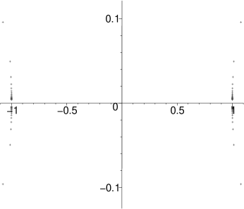
Figure 4: Roots of the function $\omega(t)$ given by Eq. (105); here $t$ is measured in units of $T$. The roots form sequences that accumulate around $t=\pm T$ and curve away from $t=0$ if $\left|A\right|<1$.

For the numerical calculation, we chose $\omega_{0}=1$, $T=8$, and $A=0.1$. The results are given in Fig. 5 and Table 3. The computed values show that a few first terms of the WKB series can be used near $t_{0}=T$; the estimate $n_{\max}\approx 0$ is invalid in that regime.

\psfrag{t1}{1}\psfrag{t2}{2}\psfrag{t3}{3}\psfrag{t4}{4}\psfrag{t5}{5}\psfrag{t6}{6}\psfrag{t7}{7}\psfrag{sss}{$|S_{n}|/S_{0}$}\psfrag{nnn}{$n$}\includegraphics[width=180.67499pt]{terms4.eps}

Figure 5: Analogous plot as in Fig. 2 for the function $\omega(t)$ given by Eq. (105). The curves are labeled 1-7 according to the consecutive values of $t_{0}$ in Table 3. Relatively poor agreement between crosses (the estimated values of $n_{\max}$) and the numerically obtained values is due to the presence of essential singularities in $\omega(t)$.

$t_{0}$	0.0	$2.0$	$4.0$	$5.0$	$6.0$	$7.0$	$7.5$
$n_{\max}$	8.2	6.1	4.0	3.0	2.0	1.0	0.5
$\frac{S_{n_{\max}}}{S_{0}}$	5$\cdot$1$0^{-8}$	3$\cdot$1$0^{-6}$	2$\cdot$1$0^{-4}$	0.002	0.02	$0.24$	0.9

Table 3: Numerical values of the optimal truncation order and error for Fig. 5.

VI Summary

In this paper I have reviewed some aspects of the adiabatic approximation and its application to cosmological particle creation, and presented new results. It is well known that there exists a fundamental limit on the accuracy of the notion of particles in curved spacetimes, due to Heisenberg uncertainty relations BirDav82 . A quantitative investigation of this accuracy is the main focus of the present paper. I showed that the best attainable precision in the definition of particles is exponentially small and of the same order as the typical particle production expected during the same epoch. The conclusion is that the ambiguity inherent in the definition of particles is precisely due to the possibility of particle production.

The main technical issue was to obtain an explicit estimate of the highest attainable precision of the WKB approximation. I have demonstrated that the WKB approximation involves a divergent series and derived a novel formula (2) for the optimal truncation order $n_{\max}$ of that series. I also estimated the error of the optimally truncated WKB series [Eq. (3)]. The error is exponentially small since typical values of $n_{\max}$ will be large if the adiabaticity condition (5) holds. Physically, the value of $n_{\max}$ is determined by the number of oscillation periods during the time of appreciable change in the frequency $\omega(t)$. Finally, I have presented analytic and numerical examples illustrating the validity of these estimates.

Appendix A Growth of derivatives of analytic functions

Here I derive some formulae used in Sec. II.4 and IV.

By definition, an analytic function $w(\theta)$ can be represented by a Taylor series at a regular point $\theta_{0}$,

$$w(\theta_{0}+z)=\sum_{n=0}^{\infty}\frac{z^{n}}{n!}w^{(n)}(\theta_{0}),$$ (108)

and it is well known that this series converges absolutely within a circle $\left|z-\theta_{0}\right|<R_{1}$, where $R_{1}$ is the distance between the point $\theta_{0}$ and the nearest singularity of $w(\theta)$ in the complex $\theta$ plane. Suppose for simplicity that the function $w(\theta)$ has simple poles at $\theta=\theta_{j}$ with residues $-c_{j}$, and that $\theta_{1}$ is the pole nearest to $\theta_{0}$. Then we may express $w(\theta)$ as

$$w(\theta)=\frac{c_{1}}{\theta_{1}-\theta}+w_{2}(\theta),$$ (109)

where the auxiliary function $w_{2}(\theta)$ is analytic within a larger circle $\left|z-\theta_{0}\right|<R_{2}$, $R_{2}>R_{1}$. The $n$-th derivative of $w(\theta)$ is therefore

$$w^{(n)}(\theta_{0})=\frac{n!c_{1}}{\left(\theta_{1}-\theta_{0}\right)^{n+1}}+w_{2}^{(n)}(\theta_{0}).$$ (110)

The same reasoning may be applied to the function $w_{2}(\theta)$ and the result is the following asymptotic estimate for the growth of derivatives,

$$w^{(n)}(\theta_{0}) =n!\left[\frac{c_{1}}{\left(\theta_{1}-\theta_{0}\right)^{n+1}}+\frac{c_{2}}{\left(\theta_{2}-\theta_{0}\right)^{n+1}}+...\right]$$

$$\sim\frac{n!}{R_{1}^{n+1}}c_{1}\left[1+O\left(\left(R_{2}/R_{1}\right)^{n}\right)\right].$$ (111)

The estimate (111) is straightforwardly generalized to the case when $w(\theta)$ has poles of higher order, e.g.

$$w(\theta)=\frac{b_{1}}{\left(\theta_{1}-\theta\right)^{2}}+\frac{c_{1}}{\theta_{1}-\theta}+w_{2}(\theta),$$

in which case we have

$$w^{(n)}(\theta_{0})\sim\frac{n!}{R_{1}^{n}}\left((n+1)\frac{b_{1}}{R_{1}}+c_{1}\right)\left[1+O\left(\left(R_{1}/R_{2}\right)^{n}\right)\right].$$

Similar estimates can be easily obtained for the case when $w(\theta)$ has more than one pole at the same distance from the initial point $\theta_{0}$.

References

- (1) B. S. DeWitt, Phys. Rep. 19, 295 (1975).
- (2) N. Birrell and P. C. W. Davies, Quantum fields in curved space (Cambridge University Press, Cambridge, 1982).
- (3) S. A. Fulling, Aspects of quantum field theory in curved spacetime (Cambridge University Press, Cambridge, 1989).
- (4) A. A. Grib, S. G. Mamayev, and V. M. Mostepanenko, Vacuum quantum effects in strong fields (Friedmann Laboratory Publishing, St. Petersburg, 1994).
- (5) L. H. Ford, Quantum Field Theory in Curved Spacetime, Proc. IXth Jorge André Swieca Summer School, Campos do Jordão-SP, Brasil, 1997, ed. by J. C. A. Barata, A. P. C. Malbouisson, and S. F. Novaes (World Scientific, Singapore, 1998), preprint gr-qc/9707062.
- (6) T. A. Jacobson, Lectures on quantum fields in curved spacetime and the Hawking effect, Proc. summer school, Valdivia (Chile, 2002), preprint gr-qc/0308048.
- (7) V. F. Mukhanov and S. Winitzki, Introduction to quantum fields in classical backgrounds, 2004 (draft version at www.theorie.physik.uni-muenchen.de/~serge/T6/).
- (8) P. C. W. Davies, “Particles do not exist,” in Quantum theory of gravity, ed. by S. M. Christensen, p. 66 (Hilger, Bristol, 1984).
- (9) S. A. Fulling, Gen. Rel. Grav. 10, 807 (1979).
- (10) L. Parker, Phys. Rev. 183, 1057 (1969).
- (11) Ya. B. Zel’dovich and A. A. Starobinskiĭ, Sov. Phys. JETP 34, 1159 (1972), Russian original: Zh. Eksp. Teor. Fiz. 61, 2161 (1971).
- (12) T. S. Bunch, S. M. Christensen, and S. A. Fulling, Phys. Rev. D 18, 4435 (1978).
- (13) C. M. Bender, S. A. Orszag, Advanced mathematical methods for scientists and engineers (McGraw-Hill, Auckland, 1978).
- (14) O. Costin, L. Dupaigne, and M. D. Kruskal, Nonlinearity 17, 1509 (2004).
- (15) G. Dunne and T. Hall, Phys. Rev. D 60, 065002 (1999).
- (16) J. Heading, Introduction to phase integral methods (Methuen, London, 1962).
- (17) F. W. J. Olver, Asymptotics and special functions (Academic Press, New York, 1974).
- (18) R. M. Kulsrud, Phys. Rev. 106, 205 (1957).
- (19) B. Chakraborty, J. Math. Phys. 14, 188 (1973).
- (20) C. M. Bender, K. Olaussen, and P. S. Wang, Phys. Rev. D 16, 1740 (1977).
- (21) M. Robnik and V. G. Romanovski, J. Phys. A: Math. Gen. 33, 5093 (2000).
- (22) V. V. Kudryashov and Y. V. Vanne, J. Appl. Math. 2, 265 (2002).
- (23) A. Joye and C-.E. Pfister, Comm. Math. Phys. 140, 15 (1991).
- (24) J. R. Ray, J. Phys. A: Math. Gen. 13, 1969 (1980).
- (25) N. Fröman and P. O. Fröman, JWKB approximation: contributions to the theory (North-Holland, Amsterdam, 1965).
- (26) M. Robnik and L. Salasnich, J. Phys. A: Math. Gen. 30, 1719 (1997); L. Salasnich and F. Sattin, J. Phys. A: Math. Gen. 30, 7597 (1997).
- (27) R. Bellman and R. Kalaba, Quasilinearization and nonlinear boundary-value problems (Elsevier, New York, 1965).
- (28) R. Krivec, V. B. Mandelzweig, and F. Tabakin, Few-Body Systems 34, 57 (2004); R. Krivec and V. B. Mandelzweig, preprint math-ph/0406023.
- (29) K. Datta and A. Rampal, Phys. Rev. D 23, 2875 (1981).
- (30) J. Hong, A. Vilenkin, and S. Winitzki, Phys. Rev. D 68, 023520 (2003); Phys. Rev. D 68, 023521 (2003).
- (31) F. V. Atkinson, J. Math. Anal. Appl. 1, 255 (1960).
- (32) I. Kay, J. Math. Anal. Appl. 3, 40 (1961).
- (33) R. Landauer, Phys. Rev. 82, 80 (1951).
- (34) H. B. Keller and J. B. Keller, J. SIAM 10, 246 (1962).
- (35) R. B. Dingle, Asymptotic expansions: their derivation and interpretation (Academic Press, New York, 1973).