Search for gravitational waves from binary black hole inspirals in LIGO data

Abstract

We report on a search for gravitational waves from binary black hole inspirals in the data from the second science run of the LIGO interferometers. The search focused on binary systems with component masses between 3 and 20 $M_{\odot}$. Optimally oriented binaries with distances up to 1 Mpc could be detected with efficiency of at least 90%. We found no events that could be identified as gravitational waves in the 385.6 hours of data that we searched.

I Introduction

The Laser Interferometric Gravitational Wave Observatory (LIGO) Abramovici et al. (1992) consists of three Fabry-Perot-Michelson interferometers, which are sensitive to the minute changes that would be induced in the relative lengths of their orthogonal arms by a passing gravitational wave. These interferometers are nearing the end of their commissioning phase and were close to design sensitivity as of March 2005. During the four science runs that have been completed until now (first (S1) during 2002, second (S2) and third (S3) during 2003 and fourth (S4) during 2005) all three LIGO interferometers were operated stably and in coincidence. Although these science runs were performed during the commissioning phase they each represent the best broad-band sensitivity to gravitational waves that had been achieved up to that date.

In this paper we report the results of a search for gravitational waves from the inspiral phase of stellar mass binary black hole (BBH) systems, using the data from the second science run of the LIGO interferometers. These BBH systems are expected to emit gravitational waves at frequencies detectable by LIGO during the final stages of inspiral (decay of the orbit due to energy radiated as gravitational waves), the merger (rapid infall) and the subsequent ringdown of the quasi-normal modes of the resulting single black hole.

The rate of BBH coalescences in the Universe is highly uncertain. In contrast to searches for gravitational waves from the inspiral phase of binary neutron star (BNS) systems Abbott et al. (2005), it is not possible to set a reliable upper limit on astrophysical BBH coalescences. That is because the distribution of the sources in space, in the component mass space and in the spin angular momentum space is not reliably known. Additionally, the gravitational waveforms for the inspiral phase of stellar-mass BBH systems which merge in the frequency band of the LIGO interferometers are not known with precision. We perform a search that aims at detection of BBH inspirals. In the absence of a detection, we use a specific nominal model for the BBH population in the Universe and the gravitational waveforms given in the literature to calculate an upper limit for the rate of BBH coalescences.

The rest of the paper is organized as follows. Sec. II provides a short description of the data that was used for the search. In Sec. III we discuss the target sources of the search and we explain the motivation for using a family of phenomenological templates to search the data. In Sec. IV we give a detailed discussion of the templates and the filtering methods. In Sec. V.1 we provide information on various data quality checks that we performed, in Sec. V.2 we describe in detail the analysis method that we used and in Sec. V.3 we provide details on the parameter tuning. In Sec. VI we describe the estimation of the background and in Sec. VII we present the results of the search. We finally show the calculation of the rate upper limit on BBH coalescences in Sec. VIII and we provide a brief summary of the results in Sec. IX.

II Data sample

During the second science run, the three LIGO interferometers were operating in science mode (see Sec. V.1). The three interferometers are based at two observatories. We refer to the observatory at Livingston, LA, as LLO and the observatory at Hanford, WA as LHO. A total of 536 hours of data from the LLO 4 km interferometer (hereafter L1), 1044 hours of data from the LHO 4 km (hereafter H1) interferometer, and 822 hours of data from the LHO 2 km (hereafter H2) interferometer was obtained. The data was subjected to several quality checks. In this search, we used only data from times when the L1 interferometer was running in coincidence with at least one of H1 and H2, and we only used continuous data of duration longer than 2048 s (see Sec. V.2). After the data quality cuts, there was a total of 101.7 hours of L1-H1 double coincident data (when both L1 and H1 but not H2 were operating), 33.3 hours of L1-H2 double coincident data (when both L1 and H2 but not H1 were operating) and 250.6 hours of L1-H1-H2 triple coincident data (when all three interferometers were operating) from the S2 data set, for a total of 385.6 hours of data.

A fraction (approximately 9%) of this data (chosen to be representative of the whole run) was set aside as “playground” data where the various parameters of the analysis could be tuned and where vetoes effective in eliminating spurious noise events could be identified. The fact that the tuning was performed using this subset of data does not exclude the possibility that a detection could be made in this subset. However, to avoid biasing the upper limit, those times were excluded from the upper limit calculation.

As with earlier analyses of LIGO data, the output of the antisymmetric port of the interferometer was calibrated to obtain a measure of the relative strain $\Delta L/L$ of the interferometer arms, where $\Delta L=L_{x}-L_{y}$ is the difference in length between the $x$ arm and the $y$ arm and $L$ is the average arm length. The calibration was measured by applying known forces to the end mirrors of the interferometers before, after and occasionally during the science run. In the frequency band between $100$ Hz and $1500$ Hz, the calibration accuracy was within 10% in amplitude and $10^{\circ}$ of phase.

III Target Sources

The target sources for the search described in this paper are binary systems that consist of two black holes with component masses between 3 and 20 $M_{\odot}$, in the last seconds before coalescence. Coalescences of binary systems consist of three phases: the inspiral, the merger and the ringdown. We performed the search by matched filtering the data using templates for the inspiral phase of the evolution of the binaries. The exact duration of the inspiral signal depends on the masses of the binary. Given the low-frequency cutoff of $100$ Hz that needed to be imposed on the data (see Sec. V.2) the expected duration of the inspiral signals in the S2 LIGO band as predicted by post-Newtonian calculations varies from 0.607 s for a $3-3\ M_{\odot}$ binary to 0.013 s for a $20-20\ M_{\odot}$ binary.

The gravitational wave signal is dominated by the merger phase which potentially may be computed using numerical solutions to Einstein’s equations. Searching exclusively for the merger using matched-filter techniques is not appropriate until the merger waveforms are known. BBH mergers are usually searched for by using techniques developed for detection of unmodeled gravitational wave bursts Abbott et al. (2004a). However, for reasons that will be explained below, it is possible that the search described in this paper was also sensitive to at least part of the merger of the BBH systems of interest. Certain re-summation techniques have been applied to model the late time evolution of BBH systems which makes it possible to evolve those systems beyond the inspiral and into the merger phase Damour et al. (1998); Buonanno and Damour (1999, 2000); Damour et al. (2000, 2001, 2003); Blanchet et al. (2004) and the templates that we used for matched filtering incorporate the early merger features (in addition to the inspiral phase) of those waveforms.

The frequencies of the ringdown radiation from BBH systems with component masses between 3 and 20 $M_{\odot}$ range from 295 Hz to 1966 Hz Echeverria (1989); Leaver (1985); Creighton (1999) and the gravitational wave forms are known. Based on the frequencies of these signals, some of the signals are in the S2 LIGO frequency band of good sensitivity and some are not. At the time of the search presented in this paper, the matched-filtering tools necessary to search for the ringdown phase of BBH were being developed. In future searches we will look for ringdown signals associated with inspiral candidates.

Finally, we have verified through simulations that the presence of the merger and the ringdown phases of the gravitational wave signal in the data does not degrade our ability to detect the inspiral phase, when we use matched filter techniques.

III.1 Characteristics of BNS and BBH inspirals

We use the standard convention $c=G=1$ in the remainder of this paper.

The standard approach to solving the BBH evolution problem uses the post-Newtonian (PN) expansion Blanchet et al. (2004) of the Einstein equations to compute the binding energy $E$ of the binary and the flux $F$ of the radiation at infinity, both as series expansions in the invariant velocity $v$ (or the orbital frequency) of the system. This is supplemented with the energy balance equation ($dE/dt=-F$) which in turn gives the evolution of the orbital phase and hence the gravitational wave phase which, to the dominant order, is twice the orbital phase. This method works well when the velocities in the system are much smaller compared to the speed of light, $v\ll 1$. Moreover, the post-Newtonian expansion is now complete to order $v^{7}$ giving us the dynamics and orbital phasing to a high accuracy Blanchet et al. (2002); Blanchet (2002). Whether the waveform predicted by the model to such high orders in the post-Newtonian expansion is reliable for use as a matched filter depends on how relativistic the system is in the LIGO band. For the second science run of LIGO, the interferometers had very good sensitivity between 100 and 800 Hz so we calculate how relativistic BNS and BBH systems are at those two frequencies.

The velocity in a binary system of total mass M is related to the frequency $f$ of the gravitational waves by

$$v=(\pi Mf)^{1/3}.$$ (1)

When a BNS system that consists of two $1.4\,M_{\odot}$ components enters the S2 LIGO band, the velocity in the system is $v\simeq 0.16$; when it leaves the S2 LIGO band at 800 Hz, it is $v\simeq 0.33$ and the system is mildly relativistic. Thus, relativistic corrections are not too important for the inspiral phase of BNS.

BBH systems of high mass, however, would be quite relativistic in the S2 LIGO band. For instance, when a $10-10\,M_{\odot}$ BBH enters the S2 LIGO band the velocity would be $v\simeq 0.31$. At a frequency of 200 Hz (smaller than the frequency of the innermost stable circular orbit, explained below, which is 220 Hz according to the test-mass approximation) the velocity would be $v\simeq 0.40$. Such a binary is expected to merge producing gravitational waves within the LIGO frequency band. Therefore LIGO would observe BBH systems in the most non-linear regime of their evolution and thereby witness highly relativistic phenomena for which the perturbative expansion is unreliable.

Numerical relativity is not yet in a position to fully solve the late time phasing of BBH systems. For this reason, in recent years, (non-perturbative) analytical resummation techniques of the post-Newtonian series have been developed to speed up its convergence and obtain information on the late stages of the inspiral and the merger Blanchet et al. (1996). These resummation techniques have been applied to the post-Newtonian expanded conservative and non-conservative part of the dynamics and are called effective-one-body (EOB) and P-approximants (also referred to as Padé approximants) Damour et al. (1998); Buonanno and Damour (1999, 2000); Damour et al. (2000, 2001, 2003). Some insights into the merger problem have been also provided in Baker et al. (2002a, b) by combining numerical and perturbative approximation schemes.

The amplitude and the phase of the standard post-Newtonian (TaylorT3, Blanchet et al. (1996)), EOB, and Padé waveforms, evaluated at different post-Newtonian orders, differ from each other in the last stages of inspiral, close to the innermost stable circular orbit (ISCO, Blanchet et al. (1996)). The TaylorT3 and Padé waveforms are derived assuming that the two black holes move along a quasi-stationary sequence of circular orbits. The EOB waveforms, extending beyond the ISCO, contain features of the merger dynamics. All those model-based waveforms are characterized by different ending frequencies. For the quasi-stationary two-body models the ending frequency is determined by the minimum of the energy. For the models that extend beyond the ISCO, the ending frequency is fixed by the light-ring Buonanno and Damour (2000); Buonanno et al. (2003a) of the two-body dynamics.

We could construct matched filters using waveforms from each of these families to search for BBH inspirals but yet the true gravitational wave signal might be “in between” the models we search for. In order not to miss the true gravitational wave signal it is desirable to search a space that encompasses all the different families and to also search the space “in between” them.

III.2 Scope of the search

Recent work by Buonanno, Chen and Vallisneri Buonanno et al. (2003a) (hereafter BCV) has unified the different approximation schemes into one family of phenomenological waveforms by introducing two new parameters, one of which is an amplitude correction factor and the other a variable frequency cutoff, in order to model the different post-Newtonian approximations and their variations. Additionally, in order to achieve high signal-matching performance, they introduced unphysical parameters in the phase evolution of the waveform.

In this work we used a specific implementation of the phenomenological templates. As these phenomenological waveforms are not guaranteed to have a good overlap with the true gravitational wave signal it is less meaningful to set upper limits on either the strength of gravitational waves observed during our search or on the coalescence rate of BBH in the Universe than it was for the BNS search in the S2 data Abbott et al. (2005). However, in order to give an interpretation of the result of our search, we did calculate an upper limit on the coalescence rate of BBH systems, based on two assumptions: (1) that the model-based waveforms that exist in the literature have good overlap with a true gravitational wave signal and (2) that the phenomenological templates used have a good overlap with the majority of the model-based BBH inspiral waveforms proposed in the literature Buonanno et al. (2003a).

To set the stage for later discussion we plot in Fig. 1 the distance at which a binary of two components of equal mass that is optimally oriented (positioned directly above the interferometer and with its orbital plane perpendicular to the line of sight from the interferometer to the binary) would produce a signal-to-noise ratio (SNR, see Sec. IV) of $8$ in the LIGO interferometers during the second science run. We refer to this distance as “range” of the interferometers. The solid line shows the range of the LIGO interferometers for matched filtering performed with the standard post-Newtonian (TaylorT3) waveforms, which predict the evolution of the system up to the ISCO Blanchet et al. (1996), at a gravitational wave frequency of $f_{\rm GW}\sim 110\left(M/40M_{\odot}\right)^{-1}$ Hz. The dashed line shows the range of the interferometers for matched filtering performed with the EOB waveforms, which predict the evolution of the system up to the light ring orbit Buonanno and Damour (2000); Buonanno et al. (2003a), at a gravitational wave frequency of $f_{\rm GW}\sim 218\left(M/40M_{\odot}\right)^{-1}$ Hz (notice that both these equations for $f_{\rm GW}$ are for binaries of equal component masses). Since the EOB waveforms extend beyond the ISCO, they have longer duration and greater energy in the LIGO band which explains why the range for the EOB waveforms is greater than the range for the TaylorT3 or Padé waveforms (calculations performed with the Padé waveforms result in ranges similar to those given by the TaylorT3 waveforms).

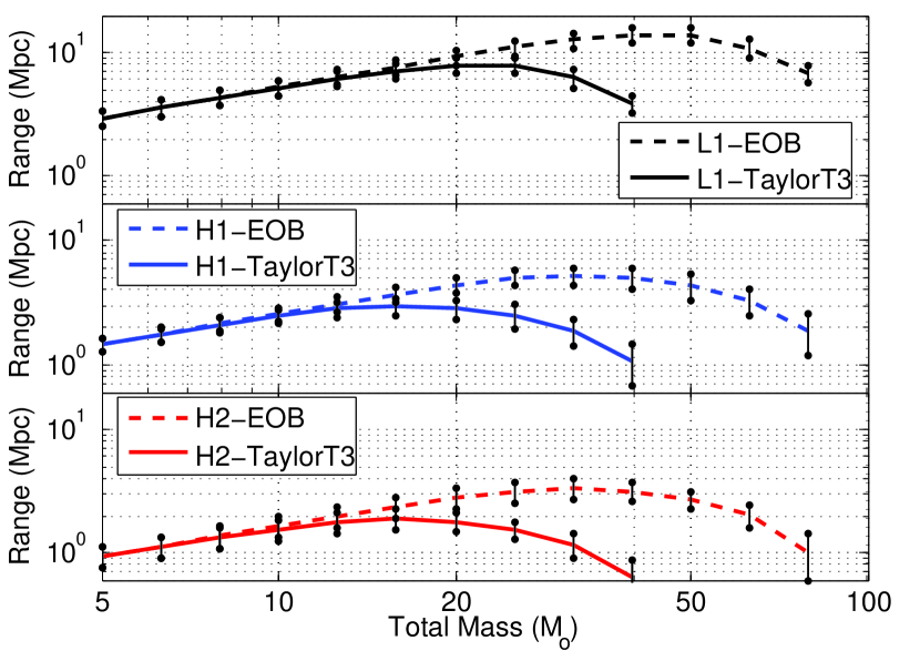
Figure 1: Range (distance at which an optimally oriented inspiraling binary of given total mass would produce a signal-to-noise ratio of $8$) of the LIGO interferometers during S2. The error bars are calculated from the fluctuations of the noise in the LIGO interferometers during S2.

During S2 the L1 interferometer was the most sensitive with a range of $7$ Mpc for a $10-10\,M_{\odot}$ binary (calculated using the TaylorT3 waveform). However, since for the search described in this paper we demanded that our candidate events are seen in coincidence between the two LIGO observatories (as described in Sec. V.2) the overall range of the search was determined by the less sensitive LHO interferometers and thus was smaller than this maximum.

IV Filtering

IV.1 Detection template family

As was mentioned in Sec. III, the gravitational wave signal from inspiraling black hole binaries of high masses enters the LIGO frequency sensitivity band in the later stages, when the post-Newtonian approximation is beginning to lose validity and different versions of the approximation are beginning to substantially differ from each other. In order to detect these inspiral signals we need to use filters based on phenomenological waveforms (instead of model-based waveforms) that cover the function space spanned by different versions of the late-inspiral post-Newtonian approximation.

It must be emphasized at this point that black hole binaries with small component masses (corresponding to total mass up to 10 $M_{\odot}$) enter the S2 LIGO sensitivity band at an early enough stage of the inspiral that the signal can be adequately approximated by the stationary phase approximation to the standard post-Newtonian approximation. For those binaries it is not necessary to use phenomenological templates for the matched filtering; the standard post-Newtonian waveforms can be used as in the search for BNS inspirals. However, using the phenomenological waveforms for those binaries does not limit the efficiency of the search Buonanno et al. (2003a). In this search, in order to treat all black hole binaries uniformly, we chose to use the BCV templates with parameters that span the component mass range from 3 to 20 $M_{\odot}$.

The phenomenological templates introduced in Buonanno et al. (2003a) match very well most physical waveform models that have been suggested in the literature for BBH coalescences. Even though they are not derived by calculations based on a specific physical model they are inspired by the standard post-Newtonian inspiral waveforms. In the frequency domain, they are

$$\tilde{h}(f)\equiv\mathcal{A}(f)e^{i\psi(f)},\;f>0,$$ (2)

where the amplitude $\mathcal{A}(f)$ is

$$\mathcal{A}(f)\equiv f^{-7/6}\left(1-\alpha f^{2/3}\right)\theta\left(f_{\textrm{cut}}-f\right)$$ (3)

and the phase $\psi(f)$ is

$$\psi(f)\equiv\phi_{0}+2\pi ft_{0}+f^{-5/3}\sum_{n=0}^{\infty}f^{n/3}\psi_{n}.$$ (4)

In Eq. (3) $\theta$ is the Heaviside step function and in Eq. (4) $t_{0}$ and $\phi_{0}$ are offsets on the time of arrival and on the phase of the signal respectively. Also, $\alpha$, $f_{\mathrm{cut}}$ and $\psi_{n}$ are parameters of the phenomenological waveforms.

Two components can be identified in the amplitude part of the BCV templates. The $f^{-7/6}$ term comes from the restricted-Newtonian amplitude in the Stationary Phase Approximation (SPA) Droz et al. (1999); Thorne (1987); Sathyaprakash and Dhurandhar (1991). The term $\alpha f^{2/3}\times f^{-7/6}=\alpha f^{-1/2}$ is introduced to capture any post-Newtonian amplitude corrections and to give high overlaps between the BCV templates and the various models that evolve the binary past the ISCO frequency. Additionally, in order to obtain high matches with the various post-Newtonian models that predict different terminating frequencies, a cutoff frequency $f_{\mathrm{cut}}$ is imposed to terminate the waveform.

It has been shown Buonanno et al. (2003a) that in order to achieve high matches with the various model-derived BBH inspiral waveforms it is in fact sufficient to use only the parameters $\psi_{0}$ and $\psi_{3}$ in the phase expression in Eq. (4), if those two parameters are allowed to take unphysical values. Thus, we set all other $\psi_{n}$ coefficients equal to 0 and simplify the phase to

$$\psi(f) = \phi_{0}+2\pi ft_{0}+f^{-5/3}(\psi_{0}+\psi_{3}f)$$ (5)

$$\equiv \phi_{0}+\psi_{s}(f)$$ (6)

where the subscript $s$ stands for “simplified”.

For the filtering of the data, a bank of BCV templates was constructed over the parameters $f_{\text{cut}}$, $\psi_{0}$ and $\psi_{3}$ (intrinsic template parameters). For details on how the templates in the bank were chosen see Sec. V.2. For each template, the signal-to-noise ratio (defined in Sec. IV.2) is maximized over the parameters $t_{0}$, $\phi_{0}$ and $\alpha$ (extrinsic template parameters).

IV.2 Filtering and signal-to-noise ratio maximization

For a signal $s$, the signal-to-noise ratio (SNR) resulting from matched-filtering with a template $h$ is

$$\rho(h)=\frac{\left<s,h\right>}{\sqrt{\left<h,h\right>}},$$ (7)

with the inner product $\left<s,h\right>$ being

$$\left<s,h\right>=2\int_{-\infty}^{\infty}\frac{\tilde{s}(f)\tilde{h}^{\ast}(f)}{S_{h}(|f|)}df=4\Re\int_{0}^{\infty}\frac{\tilde{s}(f)\tilde{h}^{\ast}(f)}{S_{h}(f)}df$$ (8)

and $S_{h}(f)$ being the one-sided noise power spectral density.

Various manipulations (given in detail in App. A) give the expression for the SNR (maximized over the extrinsic parameters $\phi_{0}$, $\alpha$ and $t_{0}$) that was used in this search. That expression is

$$\rho_{\mathrm{maximized}} =\frac{1}{2}\sqrt{|F_{1}|^{2}+|F_{2}|^{2}+2\Im(F_{1}F_{2}^{\ast})}$$

$$+\frac{1}{2}\sqrt{|F_{1}|^{2}+|F_{2}|^{2}-2\Im(F_{1}F_{2}^{\ast})}.$$

where

$$F_{1}=\int_{0}^{f_{\mathrm{cut}}}\frac{4\tilde{s}(f)a_{1}f^{-\frac{7}{6}}}{S_{h}(f)}e^{-i\psi_{s}(f)}df$$ (10)

$$F_{2}=\int_{0}^{f_{\mathrm{cut}}}\frac{4\tilde{s}(f)(b_{1}f^{-\frac{7}{6}}+b_{2}f^{-\frac{1}{2}})}{S_{h}(f)}e^{-i\psi_{s}(f)}df.$$ (11)

The quantities $a_{1}$, $b_{1}$ and $b_{2}$ are dependent on the noise and the cutoff frequency $f_{\mathrm{cut}}$ and are defined in App. A. The original suggestion of Buonanno, Chen and Vallisneri was that for the SNR maximization over the parameter $\alpha$ the values of $(\alpha\times f_{\mathrm{cut}}^{2/3})$ should be restricted within the range $[0,\ 1]$, for reasons that will be explained in Sec. V.3.1. However, in order to be able to perform various investigations on the values of $\alpha$ we leave its value unconstrained in this maximization procedure. More details on this can be found in Sec. V.3.1.

V Search for events

V.1 Data quality and veto study

The matched filtering algorithm is optimal for data with a known calibrated noise spectrum that is Gaussian and stationary over the time scale of the data blocks analyzed ($2048$ s, described in Section V.2), which requires stable, well-characterized interferometer performance. In practice, the performance is influenced by non-stationary optical alignment, servo control settings, and environmental conditions. We used two strategies to avoid problematic data. The first strategy was to evaluate data quality over relatively long time intervals using several different tests. As in the BNS search, time intervals identified as being unsuitable for analysis were skipped when filtering the data. The second strategy was to look for signatures in environmental monitoring channels and auxiliary interferometer channels that would indicate an environmental disturbance or instrumental transient, allowing us to veto any candidate events recorded at that time.

The most promising candidate for a veto channel was L1:LSC-POB_I (hereafter referred to as “POBI”), an auxiliary channel measuring signals proportional to the length fluctuations of the power recycling cavity. This channel was found to have highly variable noise at $70$ Hz which coupled into the gravitational wave channel. Transients found in this channel were used as vetoes for the BNS search in the S2 data Abbott et al. (2005). Hardware injections of simulated inspiral signals Fairhurst et al. (2004) were used to prove that signals in POBI would not veto true inspiral gravitational waves present in the data.

Investigations showed that using the correlations between POBI and the gravitational wave channel to veto candidate events would be less efficacious than it was in the BNS search. Therefore POBI was not used a an a-priori veto. However, the fact that correlations were proven to exist between the POBI signals and the BBH inspiral signals made it worthwhile to follow-up the BBH inspiral events that resulted at the end of our analysis and check if they were correlated with POBI signals (see Sec. VII.2).

As in the BNS search in the S2 data, no instrumental vetoes were found for H1 and H2. A more extensive discussion of the LIGO S2 binary inspiral veto studies can be found in Christensen et al. (2004).

V.2 Analysis Pipeline

In order to increase the confidence that a candidate event coming out of our analysis is a true gravitational wave and not due to environmental or instrumental noise we demanded the candidate event to be present in the L1 interferometer and at least one of the LHO interferometers. Such an event would then be characterized as a potential inspiral event and be subject to thorough examination.

The analysis pipeline that was used to perform the BNS search (and was described in detail in Abbott et al. (2005)) was the starting structure for constructing the pipeline used in the BBH inspiral search described in this paper. However, due to the different nature of the search, the details of some components of the pipeline needed to be modified. In order to highlight the differences of the two pipelines and to explain the reasons for those, we describe our pipeline below.

First, various data quality cuts were applied on the data and the segments of good data for each interferometer were indentified. The times when each interferometer was in stable operation (called science segments) were used to construct three data sets corresponding to: (1) times when all three interferometers were operating (L1-H1-H2 triple coincident data), (2) times when only the L1 and H1 (and not the H2) interferometers were operating (L1-H1 double coincident data) and (3) times when only the L1 and H2 (and not the H1) interferometers were operating (L1-H2 double coincident data). The analysis pipeline produced a list of coincident triggers (times and template parameters for which the SNR threshold was exceeded and all cuts mentioned below were passed) for each of the three data sets.

The science segments were analyzed in blocks of 2048 s using the findchirp implementation Allen et al. (2005) of matched filtering for inspiral signals in the LIGO Algorithm library LAL . The original version of findchirp had been coded for the BNS search and thus had to be modified to allow filtering of the data with the BCV templates described in Sec. IV.

The data for each 2048 s block was first down-sampled from 16384 Hz to 4096 Hz. It was subsequently high-pass filtered at 90 Hz in the time domain and a low frequency cutoff of 100 Hz was imposed in the frequency domain. The instrumental response for the block was calculated using the average value of the calibration (measured every minute) over the duration of the block.

The breaking up of each segment for power spectrum estimation and for matched-filtering was identical to the BNS search Abbott et al. (2005) and is briefly mentioned here so that the terminology is established for the pipeline description that follows.

Triggers were not searched for within the first and last $64$ s of a given block, so subsequent blocks were overlapped by $128$ s to ensure that all of the data in a continuous science segment (except for the first and last 64 s) was searched. Any science segments shorter than $2048$ s were ignored. If a science segment could not be exactly divided into overlapping blocks (as was usually the case) the remainder of the segment was covered by a special $2048$ s block which overlapped with the previous block as much as necessary to allow it to reach the end of the segment. For this final block, a parameter was set to restrict the inspiral search to the time interval not covered by any previous block, as shown in Fig. 2.

Each block was further split into 15 analysis segments of length 256 s overlapped at the beginning and at the end by 64 s. The average power spectrum $S_{h}(f)$ for the 2048 s of data was estimated by taking the median of the power spectra of the 15 segments. We used the median instead of the mean to avoid biased estimates due to large outliers, produced by non-stationary data. The calibration was applied to the data in each analysis segment.

In order to avoid end-effects due to wraparound of the discrete Fourier transform when performing the matched filter, the frequency-weighting factor $1/S_{h}(f)$ was truncated in the time domain so that its inverse Fourier transform had a maximum duration of $\pm 16$ s. The output of the matched filter near the beginning and end of each segment was corrupted by end-effects due to the finite duration of the power spectrum weighting and the template. By ignoring the filter output within 64 s of the beginning and end of each segment, we ensured that only uncorrupted filter output is searched for inspiral triggers. This necessitated the overlapping of segments and blocks described above.

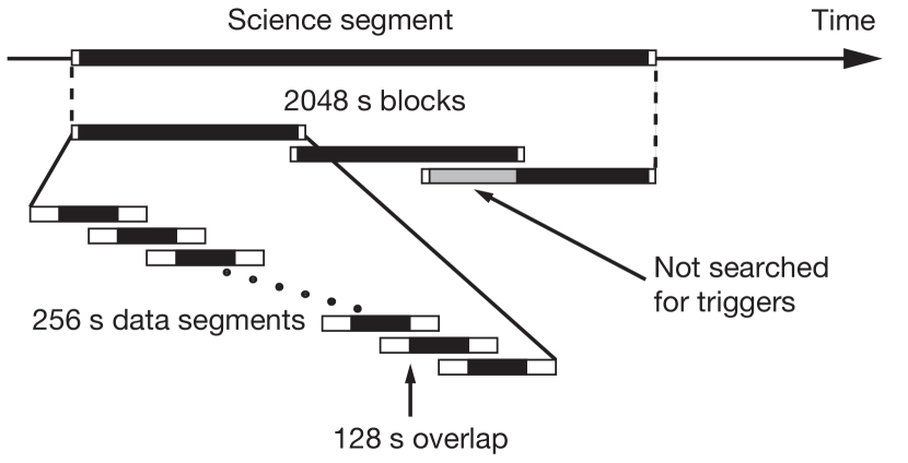
Figure 2: The algorithm used to divide science segments into data analysis segments. Science segments are divided into $2048$ s blocks overlapped by $128$ s. (Science segments shorter than $2048$ s are ignored.) An additional block with a larger overlap is added to cover any remaining data at the end of a science segment. Each block is divided into $15$ analysis sesgments of length $256$ s for filtering. The first and last $64$ s of each analysis segment are ignored, so the segments overlap by $128$ s. Areas shaded black are searched for triggers by the search pipeline. The gray area in the last block of the science segment is not searched for triggers as this time is covered by the preceding block, although these data points are used in estimating the noise power spectral density for the final block.

The single-sided power spectral density (PSD) of the noise $S_{h}(f)$ in the L1 interferometer was estimated independently for each L1 block that was coincident with operation of at least one LHO interferometer. The PSD was used to construct a template bank for filtering that block. The bank was constructed over the parameters $\psi_{0}$ and $\psi_{3}$ so that there was no less than $95\%$ overlap (defined in the sense of Eq. (A) between two neighboring (in $\{\psi_{0},\ \psi_{3},\ f_{\mathrm{cut}}\}$ parameter space) templates, if the value of $\alpha$ of those templates was equal to 0. The $\psi_{0}-\psi_{3}$ space was tiled using a square grid based on the metric in Eq. (117) of Buonanno et al. (2003a). For each pair of $\psi_{0}$ and $\psi_{3}$, three values of the cutoff frequency $f_{\mathrm{cut}}$ were generated. This process gave the three intrinsic parameters for each template. Details on the exact values of the parameters used are given in Sec. V.3.1. The number of templates in the bank varied with the PSD. For this search the number of templates ranged between 741 and 1296 templates per 2048 s L1 analysis block, with the average number being 958.

The data from the L1 interferometer for the block was then matched-filtered, as described previously, against the bank of templates, with a SNR threshold $\rho_{\mathrm{L}}^{\mathrm{thresh}}$ to produce a list of triggers. As will be explained below, the $\chi^{2}$-veto Allen (2005) that was used for the BNS search was not used in this search. For each block in the LHO interferometers, a triggered bank was created consisting of every template that produced at least one trigger in the L1 data during the time of the LHO block. This triggered bank was used to matched-filter the data from the LHO interferometers. For times when only the H2 interferometer was operating in coincidence with L1, the triggered bank was used to matched-filter the H2 blocks that overlapped with L1 data. For all other times, all H1 data that overlapped with L1 data was matched-filtered using the triggered bank for that block. For H1 triggers produced during times when all three interferometers were operating, a second triggered bank was produced for each H2 block. This triggered bank consisted of every template which produced at least one trigger found in coincidence in L1 and H1 during the time of the H2 block. The H2 block was matched-filtered with this bank.

Before any triggers were tested for coincidence, all triggers with $(\alpha\times f_{\text{cut}}^{2/3})$ greater than a threshold $\alpha_{F}^{\text{thresh}}$ were rejected. The reason for this veto will be explained in Sec. V.3.

For triggers to be considered coincident between two interferometers they had to be observed in both interferometers within a time window that allowed for the error in measurement of the time of the trigger. If the interferometers were not co-located, this parameter was increased by the light travel time between the two LIGO observatories ($10$ ms). We then ensured that the triggers had consistent waveform parameters by demanding that the two parameters $\psi_{0}$ and $\psi_{3}$ for the template were exactly equal to each other.

Triggers that were generated from the triple coincident data were required to be found in coincidence in the L1 and H1 interferometers. We searched the H2 data from these triple coincident times but did not reject L1-H1 coincident triggers that were not found in the H2 data, even if, based on the SNR observed in H1 they would be expected to be found in H2. This was a looser rejection algorithm than the one used for the BNS search Abbott et al. (2005) and could potentially increase the number of false alarms in the triple coincident data. The reason for using this algorithm in the BBH search is explained in Sec. V.3.2, where the coincidence parameter tuning is discussed.

The last step of the pipeline was the clustering of the triggers. The clustering is necessary because both large astrophysical signals and instrumental noise bursts can produce many triggers with coalescence times within a few ms of each other and with different template parameters. Triggers separated by more than 0.25 s were considered distinct. This time was approximately half of the duration of the longest signal that we could detect in this search. We chose the trigger with the largest combined SNR from each cluster, where the combined SNR is defined in Sec. VI.

To perform the search on the full data set, a Directed Acyclic Graph (DAG) was constructed to describe the work flow, and execution of the pipeline tasks was managed by Condor Tannenbaum et al. (2001) on the various Beowulf clusters of the LIGO Scientific Collaboration. The software to perform all steps of the analysis pipeline and construct the DAG is available in the package lalapps LAL .

V.3 Parameter Tuning

An important part of the analysis was to decide on the values of the various parameters of the search, such as the SNR thresholds and the coincidence parameters. The parameters were chosen so as to compromise between increasing the detection efficiency and lowering the number of false alarms.

The tuning of all the parameters was done by studying the playground data only. In order to tune the parameters we performed a number of Monte-Carlo simulations, in which we added simulated BBH inspiral signals in the data and searched for them with our pipeline. While we used the phenomenological detection templates to perform the matched filtering, we used various model-based waveforms for the simulated signals that we added in the data. Specifically, we chose to inject effective-one-body (EOB, Damour et al. (1998); Buonanno and Damour (1999, 2000); Damour et al. (2001)), Padé (PadéT1, Damour et al. (1998)) and standard post-Newtonian waveforms (TaylorT3, Blanchet et al. (1996)), all of second post-Newtonian order. Injecting waveforms from different families allowed us to additionally test the efficiency of the BCV templates for recovering signals predicted by different models.

In contrast to neutron stars, there are no observation-based predictions about the population of BBH systems in the Universe. For the purpose of tuning the parameters of our pipeline we decided to draw the signals to be added in the data from a population with distances between 10 kpc and 20 Mpc from the Earth. The random sky positions and orientations of the binaries resulted in some signals having much larger effective distances (distance from which the binary would give the same signal in the data if it were optimally oriented). It was determined that using a uniform-distance or uniform-volume distribution for the binaries would overpopulate the larger distances (for which the LIGO interferometers were not very sensitive during S2) and only give a small number of signals in the small-distance region, which would be insufficient for the parameter tuning. For that reason we decided to draw the signals from a population that was uniform in $\log$(distance). For the mass distribution, we limited each component mass between 3 and 20 $M_{\odot}$. Populations with uniform distribution of total mass were injected for the tuning part of the analysis.

There were two sets of parameters that we could tune in the pipeline: the single interferometer parameters, which were used in the matched filtering to generate inspiral triggers in each interferometer, and the parameters which were used to determine if triggers from different interferometers were coincident. The single interferometer parameters that needed to be tuned were the ranges of values for $\psi_{0}$ and $\psi_{3}$ in the template bank, the number of $f_{\mathrm{cut}}$ frequencies for each pair of $\{\psi_{0},\psi_{3}\}$ in the template bank and the SNR threshold $\rho^{\mathrm{thresh}}$. The coincidence parameters were the time coincidence window for triggers from different interferometers, $\delta t$, and the coincidence window for the template parameters $\psi_{0}$ and $\psi_{3}$. Due to the nature of the triggered search pipeline, parameter tuning was carried out in two stages. We first tuned the single interferometer parameters for the primary interferometer (L1). We then used the triggered template banks (generated from the L1 triggers) to explore the single interferometer parameters for the less sensitive LHO interferometers. Finally the parameters of the coincidence test were tuned.

V.3.1 Single interferometer tuning

Based on the playground injection analysis it was determined that the range of values for $\psi_{0}$ had to be $[10,\ 550000]\ \mathrm{Hz}^{5/3}$ and the range of values for $\psi_{3}$ had to be $[-4000,\ -10]\ \mathrm{Hz}^{2/3}$ in order to have high detection efficiency for binaries of total mass between 6 and 40 $M_{\odot}$.

Our numerical studies showed that using between 3 and 5 cutoff frequencies per $\{\psi_{0},\ \psi_{3}\}$ pair would yield very high detection efficiency. Consideration of the computational cost of the search led us to use 3 cutoff frequencies per pair, thus reducing the number of templates in each bank by 40% compared to a template bank with 5 cutoff frequencies per $\{\psi_{0},\ \psi_{3}\}$ pair.

Our Monte-Carlo simulations showed that, in order to be able to distinguish an inspiral signal from an instrumental or environmental noise event in the data, the minimum requirement should be that the trigger has SNR of at least $7$ in each interferometer. A threshold of 6 (that was used in the BNS search) resulted in a very large number of noise triggers that needlessly complicated the data handling and post-pipeline processing.

A standard part of the matched-filtering process is the $\chi^{2}$-veto Allen (2005). The $\chi^{2}$-veto compares the SNR accumulated in each of a number of frequency bands of equal inspiral template power to the expected amount in each band. Gravitational waves from inspiraling binaries give small $\chi^{2}$ values while instrumental artifacts give high $\chi^{2}$ values. Thus, the triggers resulting from instrumental artifacts can be vetoed by requiring the value of $\chi^{2}$ for a trigger to be below a threshold. The test is very efficient at distinguishing BNS inspiral signals from loud non-Gaussian noise events in the data and was used in the BNS inspiral search Abbott et al. (2005) in the S2 data. However, we found that the $\chi^{2}$-veto was not suitable for the search for gravitational waves from BBH inspirals in the S2 data. The expected short duration, low bandwidth and small number of cycles in the S2 LIGO frequency band for many of the possible BBH inspiral signals made such a test unreliable unless a very high threshold on the values of $\chi^{2}$ were to be set. A high threshold, on the other hand, resulted in only a minimal reduction in the number of noise events picked up. Additionally the $\chi^{2}$-veto is computationally very costly. We thus decided to not use it in this search.

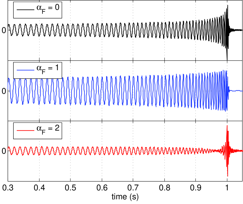
Figure 3: Time domain plots of BCV waveforms for different values of $\alpha_{F}$. The top plot is for $\alpha_{F}=0$, the middle is for $\alpha_{F}=1$ and the bottom is for $\alpha_{F}=2$. For all three waveforms $\psi_{0}=150000\ \mathrm{Hz}^{5/3}$, $\psi_{3}=-1500\ \mathrm{Hz}^{2/3}$ and $f_{\mathrm{cut}}=500$ Hz. It can be seen that the behavior is not that of a typical inspiral waveform for $\alpha_{F}=2$.

As mentioned earlier, the SNR calculated using the BCV templates was maximized over the template parameter $\alpha$. For every value of $\alpha$, there is a frequency $f_{0}$ for which the amplitude factor $(1-\alpha f^{2/3})$ becomes zero:

$$f_{0}=\alpha^{-3/2}.$$ (12)

If the value of $\alpha$ associated with a trigger is such that the frequency $f_{0}$ is greater than the cutoff frequency $f_{\mathrm{cut}}$ of the template (and consequently $\alpha\ f_{\mathrm{cut}}^{2/3}\leq 1$), then the high-frequency behavior of the phenomenological template is as expected for an inspiral gravitational waveform. If the value of $\alpha$ is such that $f_{0}$ is smaller than the cutoff frequency $f_{\mathrm{cut}}$ (and consequently $\alpha\ f_{\mathrm{cut}}^{2/3}>1$), the amplitude of the phenomenological waveform becomes zero before the cutoff frequency is reached. For such a waveform, the high-frequency behavior does not resemble that of a typical inspiral gravitational waveform. For simplicity we define

$$\alpha_{F}\equiv\alpha f_{\mathrm{cut}}^{2/3}.$$ (13)

The behavior of the BCV waveforms for three different values of $\alpha_{F}$ is shown in Fig. 3, where it can be seen that for the case of $\alpha_{F}=2$ the amplitude becomes zero and then increases again.

Despite that fact, many of the simulated signals that we added in the data were in fact recovered with values of $\alpha_{F}>1$, with a higher SNR than the SNR they would have been recovered with, had we imposed a restriction on $\alpha$. Additionally some signals gave SNR smaller than the threshold for all values of $\alpha$ that gave $\alpha_{F}\leq 1$. Multiple studies showed that this was due to the fact that we only had a limited number of cutoff frequencies in our template bank and in many cases the lack of the appropriate ending frequency was compensated for by a value of $\alpha$ that corresponded to an untypical inspiral gravitational waveform.

We performed various investigations which showed that rejecting triggers with $\alpha_{F}>1$ allowed us to still have a very high efficiency in detecting BBH inspiral signals (although not as high as if we did not impose that cut) and the cut primarily affected signals that were recovered with SNR close to the threshold. It was also proven that such a cut reduced the number of noise triggers significantly, so that the false-alarm probability was significantly reduced as well. The result was that such a cut provided a clearer distinction between the noise triggers that resulted from our pipeline and the triggers that came from simulated signals injected in the data. In order to increase our confidence in the triggers that came out of the pipeline being BBH inspiral signals, we rejected all triggers with $\alpha_{F}>1$ in this search.

As mentioned in Sec. IV, the initial suggestion of Buonanno, Chen and Vallisneri was that the parameter $\alpha_{F}$ be constrained from below to not take values less than zero. This suggestion was based on the fact that for values of $\alpha<0$, the amplitude factor $(1-\alpha f_{\mathrm{cut}}^{2/3})$ can substantially deviate from the predictions of the post-Newtonian theory at high frequencies. Investigations similar to those described for the cut $\alpha_{F}\leq 1$ did not justify rejecting the triggers with $\alpha_{F}<0$, so we set no low threshold for $\alpha_{F}$.

V.3.2 Coincidence parameter tuning

After the single interferometer parameters had been selected, the coincidence parameters were tuned using the triggers from the single interferometers.

The time of arrival of a simulated signal at an interferometer could be measured within $\pm 10$ ms. Since the H1 and H2 interferometers are co-located, $\delta t$ was chosen to be $10$ ms for H1-H2 coincidence. Since the light-travel time between the two LIGO observatories is $10$ ms, $\delta t$ was chosen to be $20$ ms for LHO-LLO coincidence.

Because we performed a triggered search, the data from all three LIGO interferometers was filtered with the same templates for each 2048 s segment. That led us to set the values for the template coincidence parameters $\Delta\psi_{0}$ and $\Delta\psi_{3}$ equal to $0$. We found that that was sufficient for the simulated BBH inspiral signals to be recovered in coincidence.

The slight misalignment of the L1 interferometer with respect to the LHO interferometers led us to choose to not impose an amplitude cut in triggers that came from the two different observatories. This choice was identical to the choice made for the BNS search Abbott et al. (2005).

We considered imposing an amplitude cut on the triggers that came from triple coincident data and were otherwise coincident between H1 and H2. A similar cut was imposed on the equivalent triggers in the BNS search. The cut relied on the calculation of the “BNS range” for H1 and H2. The BNS range is defined as the distance at which an optimally oriented neutron star binary, consisting of two components each of 1.4 $M_{\odot}$, would be detected with a SNR of 8 in the data. The value of the range depends on the PSD. For binary neutron stars the value of the range can be calculated for the 1.4-1.4 $M_{\odot}$ binary and then be rescaled for all masses. That is because the BNS inspiral signals always terminate at frequencies above 733 Hz (ISCO frequency for a 3-3 $M_{\odot}$ binary, according to the test-mass approximation) and thus for BNS the larger part of the SNR comes from the high-sensitivity band of LIGO. For black hole binaries, on the other hand, the ending frequency of the inspiral varies from 110 Hz for a 20-20 $M_{\odot}$ binary up to 733 Hz for a 3-3 $M_{\odot}$ binary (according to the test-mass approximation). That means that the range depends not only on the PSD but also on the binary that is used to calculate it. That can make a cut based on the range very unreliable and force rejection of triggers that should not be rejected. In order to be sure that we would not miss any BBH inspiral signals, we decided to not impose the amplitude consistency cut between H1 and H2.

VI Background Estimation

We estimated the rate of accidental coincidences (also known as background rate) for this search by introducing an artificial time shift $\Delta t$ to the triggers coming from the L1 interferometer relative to the LHO interferometers. The time-shift triggers were fed into the coincidence steps of the pipeline and, for the triple coincident data, to the step of the filtering of the H2 data and the H1-H2 coincidence. By choosing a shift larger than 20 ms (the time coincidence window between the two observatories), we ensured that a true gravitational wave could never produce coincident triggers in the time-shifted data streams. To avoid correlations, we used shifts longer than the duration of the longest waveform that we could detect (0.607 s given the low-frequency cutoff imposed, as explained in Sec. III). We chose to not time-shift the data from the two LHO interferometers relative to one another since there could be true correlations producing accidental coincidence triggers due to environmental disturbances affecting both of them. The resulting time-shift triggers corresponded only to accidental coincidences of noise triggers. For a given time shift, the triggers that emerged from the pipeline were considered as one single trial representation of an output from a search if no signals were present in the data.

A total of 80 time-shifts were performed and analyzed in order to estimate the background. The time shifts ranged from $\Delta t=-407\;s$ up to $\Delta t=+407\;s$ in increments of $10\;s$. The time shifts of $\pm 7s$ were not performed.

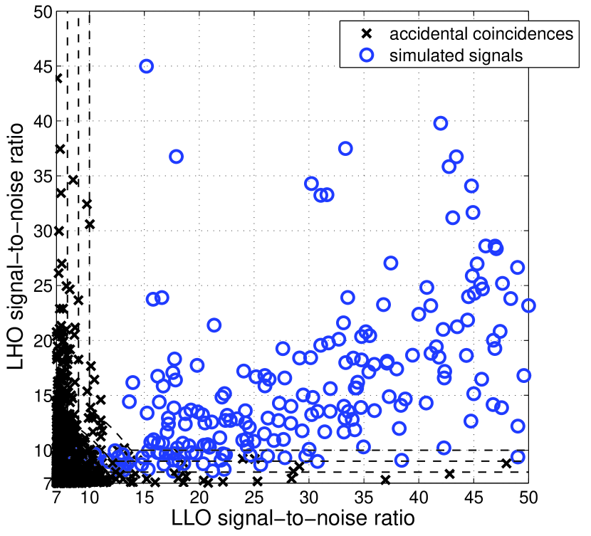
Figure 4: The LLO and LHO SNRs of the accidental coincidences from the time-shifted triggers (crosses) and the triggers from the simulated signal injections (circles) are shown. The dashed lines show the equal false-alarm contours.

VI.1 Distribution of background events

Fig. 4 shows the time shift triggers that resulted from our pipeline (crosses) in the LHO SNR $(\rho_{\mathrm{H}})$ versus the LLO SNR $(\rho_{\mathrm{L}})$ plane. There were only double coincident triggers in both the double and triple coincident data. Specifically, all the triggers present in the triple coincident data were L1-H1 coincident and were not seen in H2. Thus, $\rho_{\mathrm{H}}$ is defined as the SNR of either H1 or H2, depending on which of the three S2 data sets described in Sec. V.2 the trigger came from.

There is a group of triggers at the lower left corner of the plot, which correspond to coincidences with SNR of no more than $15$ in each observatory. There are also long “tails” of triggers which have high SNR (above 15) in one of the interferometers and low SNR (below 10) in the other. The distribution is quite different from the equivalent distribution that was observed in the BNS search Abbott et al. (2005). The presence of the tails (and their absence from the corresponding distribution in the BNS search) can be attributed to the fact that the $\chi^{2}$-veto was not applied in this search and thus some of the loud noise events that would have been eliminated by that test have instead survived.

For comparison, the triggers from some recovered injected signals are also plotted in Fig. 4 (circles). The distribution of those triggers is quite different from the distribution of the triggers resulting from accidental coincidences of noise events. The noise triggers are concentrated along the two axes of the ($\rho_{L},\ \rho_{H}$) plane and the injection triggers are spread in the region below the equal-SNR diagonal line of the same plane. This distribution of the injection triggers is due to the fact that during the second science run the L1 interferometer was more sensitive than the LHO interferometers. Consequently, a true gravitational wave signal that had comparable LLO and LHO effective distances would be observed with higher SNR in LLO than in LHO. The few injections that produced triggers above the diagonal of the graph correspond to BBH systems that are better oriented for the LHO interferometers than for the L1 interferometer, and thus have higher SNR at LHO than at LLO.

VI.2 Combined SNR

We define a “combined SNR” for the coincident triggers that come out of the time-shift analysis. The combined SNR is a statistic based on the accidental coincidences and is defined so that the higher it is for a trigger, the less likely it is that the trigger is due to an accidental coincidence of single-interferometer uncorrelated noise triggers. Looking at the plot of the $\rho_{\mathrm{H}}$ versus the $\rho_{\mathrm{L}}$ of the background triggers we notice that the appropriate contours for the triggers at the lower left corner of the plot are concentric circles with the center at the origin. However, for the tails along the axes the appropriate contours are “L” shaped. The combination of those two kinds of contours gives the contours plotted with dashed lines in Fig. 4. Based on these contours, we define the combined SNR of a trigger to be

$$\rho_{\mathrm{C}}=\min\{\sqrt{\rho_{\mathrm{L}}^{2}+\rho_{\mathrm{H}}^{2}},\;2\rho_{\mathrm{H}}-3,\;2\rho_{\mathrm{L}}-3\}.$$ (14)

After the combined SNR is assigned to each pair of triggers, the triggers are clustered by keeping the one with the highest combined SNR within 0.25 s, thus keeping the “highest confidence” trigger for each event.

VII Results

In this section we present the results of the search in the S2 data with the pipeline described in Sec. V.2. The combined SNR was assigned to the candidate events according to Eq. (14).

VII.1 Comparison of the unshifted triggers to the background

There were 25 distinct candidate events that survived all the analysis cuts. Of those, 7 were in the L1-H1 double coincident data, 10 were in the L1-H2 double coincident data and 8 were in the L1-H1-H2 triple coincident data. Those 8 events appeared only in the L1 and H1 data streams and even though they were not seen in H2 they were still kept, according to the procedure described in Sec. V.2.

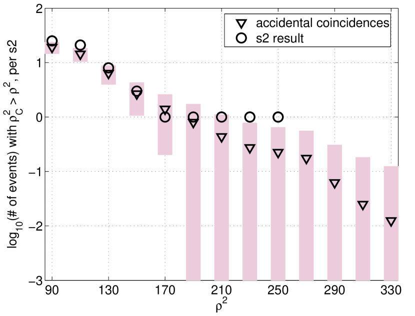
Figure 5: Expected accidental coincidences per S2 (triangles) with one standard deviation bars. The number of events in the S2 (circles) is overlayed.

In order to determine if there was an excess of candidate events above the background in the S2 data, we compared the number of zero-shift events to the expected number of accidental coincidences in S2, as predicted by the time-shift analysis described in Sec. VI. Fig. 5 shows the mean cumulative number of accidental coincidences (triangles) versus the combined SNR squared of those accidental coincidences. The bars indicate one standard deviation. The cumulative number of candidate events in the zero-shift S2 data is overlayed (circles). It is clear that the candidate events are consistent with the background.

VII.2 Investigations of the zero-shift candidate events

Even though the zero-shift candidate events are consistent with the background, we investigated them carefully. We first looked at the possibility of those candidate events being correlated with events in the POBI channel, for the reasons described in Sec. V.1.

It was determined that the loudest candidate event and three of the remaining candidate events that resulted from our analysis were coincident with noise transients in POBI. That led us to believe that the source of these candidate events was instrumental and that they were not due to gravitational waves. The rest of the candidate events were indistinguishable from the background events.

VII.3 Results of the Monte-Carlo simulations

As mentioned in Sec. V.2, the Monte-Carlo simulations allow us not only to tune the parameters of the pipeline, but also to measure the efficiency of our search method. In this section we look in detail at the results of Monte-Carlo simulations in the full data set of the second science run.

Due to the lack of observation-based predictions for the population of BBH systems in the Universe, the inspiral signals that we injected were uniformly distributed in $\log$(distance), with distance varying from 10 kpc to 20 Mpc and uniformly distributed in component mass (this mass distribution was proposed by Belczynski et al. (2002)), with each component mass varying between 3 and 20 $M_{\odot}$.

Fig. 6 shows the efficiency of recovering the injected signals (number of found injections of a given effective distance divided by the total number of injections of that effective distance) versus the injected LHO-effective distance. We chose to plot the efficiency versus the LHO-effective distance rather than versus the LLO-effective distance since H1 and H2 were less sensitive than L1 during S2.

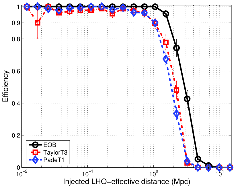
Figure 6: The efficiency versus the LHO-effective distance for the different families of injected waveforms is shown. The dashed line represents the efficiency for PadéT1 injections, the dotted line represents the efficiency for standard post-Newtonian time-domain waveforms and the solid line represents the efficiency for effective-one-body waveforms. All injected waveforms were of second post-Newtonian order. Binomial error bars are shown.

Our analysis method had efficiency of at least $90\%$ for recovering BBH inspiral signals with LHO-effective distance less than 1 Mpc for the mass range we were exploring. It should be noted how the efficiency of our pipeline varied for different injected waveforms. It is clear from Fig. 6 that the efficiency for recovering EOB waveforms was higher than that for TaylorT3 or PadéT1 waveforms for all distances. This is expected because the EOB waveforms have more power (longer duration and larger number of cycles) in the LIGO frequency band compared to the PadéT1 and TaylorT3 waveforms.

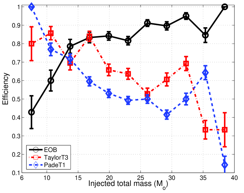
Figure 7: The efficiency versus the injected total mass of all injected signals with LHO-effective distance between 1 and 3 Mpc for the different families of injected waveforms is shown. The dashed line represents the efficiency for PadéT1 injections, the dotted line represents the efficiency for standard post-Newtonian time-domain waveforms and the solid line represents the efficiency for effective-one-body waveforms. All injected waveforms were of second post-Newtonian order. Binomial error bars are shown.

Even though the main determining factor of whether a simulated signal is recovered or not is its effective distance in the least sensitive interferometer, it is worth investigating the efficiency of recovering injections as a function of the injected total mass. In order to limit the effect of the distance in the efficiency, we chose all the injections with LHO-effective distance between 1 and 3 Mpc and plotted the efficiency versus total mass in Fig. 7. The plot shows a decrease in the detection efficiency as the total mass increases, for the TaylorT3 and the PadéT1 waveforms, but not for the EOB waveforms. The reason for this is the same as the one mentioned previously. For the TaylorT3 and the PadéT1 waveforms, the higher the total mass of the binary system, the fewer the cycles in the LIGO band. That leads to the reduction in efficiency for those waveforms. The EOB waveforms, on the other hand, extend beyond the ISCO and thus have more cycles in the LIGO band than the TaylorT3 or the PadiéT1 waveforms. The power of the signal in band is sufficient for those waveforms to be detected with an approximately equal probability for the higher masses.

VIII Upper limit on the rate of BBH inspirals

As was mentioned previously, a reliable upper limit cannot be calculated for the rate of BBH inspirals as was calculated for the rate of BNS inspirals. The reason for this is two-fold. Firstly, the characteristics of the BBH population (such as spatial, mass and spin distributions) are not known, since no BBH systems have ever been observed. In addition, the BCV templates are not guaranteed to have a good overlap with the true BBH inspiral gravitational wave signals. However, work by various groups has given insights on the possible spatial distribution and mass distribution of BBH systems Belczynski et al. (2002). Assuming that the model-based inspiral waveforms proposed in the literature have good overlap with a true inspiral gravitational wave signal and because the BCV templates have a good overlap with those model-based BBH inspiral waveforms, we used some of those predictions to give an interpretation of the result of our search.

VIII.1 Upper limit calculation

Following the notation used in Abbott et al. (2004b), let $\mathcal{R}$ indicate the rate of BBH coalescences per year per Milky Way Equivalent Galaxy (MWEG) and $N_{\mathrm{G}}(\rho^{\ast})$ indicate the number of MWEGs which our search probes at $\rho\geq\rho^{\ast}$. The probability of observing an inspiral signal with $\rho>\rho^{\ast}$ in an observation time $T$ is

$$P(\rho>\rho^{\ast};{\mathcal{R}})=1-e^{-{\mathcal{R}}TN_{\mathrm{G}}(\rho^{\ast})}.$$ (15)

A trigger can arise from either an inspiral signal in the data or from background. If $P_{b}$ denotes the probability that all background triggers have SNR less than $\rho^{\ast}$, then the probability of observing one or more triggers with $\rho>\rho^{\ast}$ is

$$P(\rho>\rho^{\ast};{\mathcal{R}},b)=1-P_{b}e^{-{\mathcal{R}}TN_{\mathrm{G}}(\rho^{\ast})}.$$ (16)

Given the probability $P_{b}$, the total observation time $T$, the SNR of the loudest event $\rho_{\mathrm{max}}$, and the number of MWEGs $N_{\mathrm{G}}(\rho_{\mathrm{max}})$ to which the search is sensitive, we find that a frequentist upper limit, at 90% confidence level, is

$${\cal R}<{\cal R}_{90\%}=\frac{2.303+\ln P_{b}}{TN_{\mathrm{G}}(\rho_{\mathrm{max}})}.$$ (17)

For ${\mathcal{R}}>{\mathcal{R}}_{90\%}$, there is more than $90\%$ probability that at least one event would be observed with SNR greater than $\rho_{\mathrm{max}}$. Details of this method of determining an upper limit can be found in Brady et al. (2004). In particular, one obtains a conservative upper limit by setting $P_{b}=1$. We adopt this approach below because of uncertainties in our background estimate.

During the 350.4 hours of non-playground data used in this search, the highest combined SNR that was observed was 16.056. The number $N_{\mathrm{G}}$ can be calculated, as in the BNS search Abbott et al. (2005), using the Monte-Carlo simulations that were performed. The difference from the BNS search is that the injected signals were not drawn from an astrophysical population, but from a population that assumes a uniform $\log$(distance) distribution. The way this difference is handled is explained below.

Our model for the BBH population carried the following assumptions:

(1) Black holes of mass between 3 and 20 $M_{\odot}$ result exclusively from the evolution of stars, so that our BBH sources are present only in galaxies.

(2) The field population of BBHs is distributed amongst galaxies in proportion to the galaxies’ blue light (as was assumed for BNS systems Abbott et al. (2005)).

(3) The component mass distribution is uniform, with values ranging from 3 to 20 $M_{\odot}$ Belczynski et al. (2002); Bulik et al. (2004).

(4) The component spins are negligibly small.

(5) The waveforms are an equal mixture of EOB, PadéT1 and TaylorT3 waveforms.

(6) The sidereal times of the coalescences are distributed uniformly throughout the S2 run.

Assumption (4) was made because the BCV templates used in this search were not intended to capture the amplitude modulations of the gravitational waveforms expected to result from BBH systems with spinning components. However, studies performed by BCV Buonanno et al. (2003b) showed that the BCV templates do have high overlaps (90% on average, the average taken over one thousand initial spin orientations) with waveforms of spinning BBH systems of comparable component masses. Templates that are more suitable for detection of spinning BBH have been developed Buonanno et al. (2003b) (BCV2) and are being used in a search for the inspiral of such binaries in the S3 LIGO data.

Assumption (5) was probably the most ad-hoc assumption in our upper limit calculation. Since this calculation was primarily intended to be illustrative of how our results can be used to set an upper limit, the mix of the waveforms was chosen for simplicity. It should be apparent how to modify the calculation to fit a different population model.

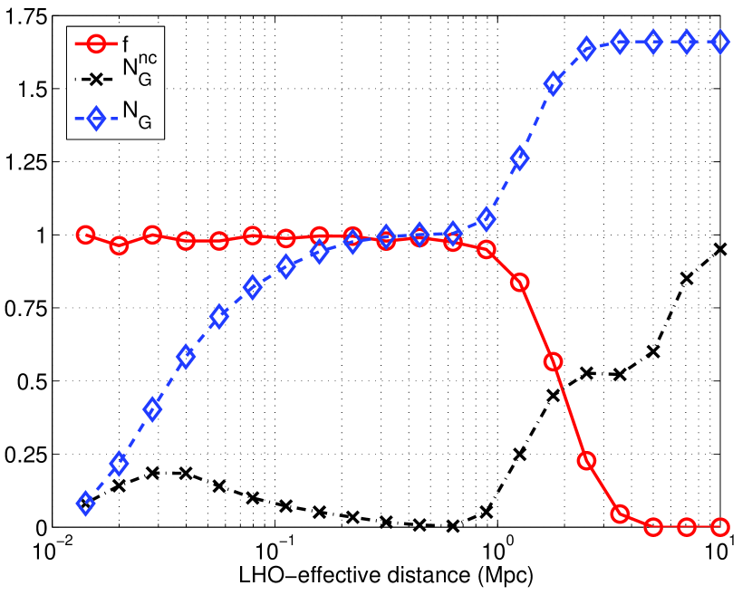
Figure 8: The number of Milky Way equivalent galaxies (crosses) and the efficiency of the search (circles) as calculated by Eq. (VIII.1) versus the LHO-effective distance (in Mpc) are shown. The cumulative number of MWEGs $N_{\mathrm{G}}$ (diamonds) versus LHO effective distance is overlayed. The horizontal axis has a logarithmic scale, in accordance with the uniform-$\log$ distance distribution of the injected BBH inspiral signals. No units are given for the vertical axis because it corresponds to three different quantities plotted against LHO-effective distance.

With assumptions (1) and (2) we determined the number of MWEGs in each logarithmic bin of LHO-effective distance ($N_{\mathrm{G}}^{\mathrm{nc}}$, crosses in Fig. 8). We used our Monte-Carlo simulations to determine the efficiency for detection of a source at LHO-effective distance $d$ with combined SNR $\rho_{\mathrm{C}}>\rho_{\mathrm{max}}$, $\rho_{\mathrm{max}}$ being the combined SNR of the loudest event observed in our search. Specifically, we define

$$f(d;\rho_{\mathrm{max}}) =\frac{1}{3}\Big{[}\frac{N_{\mathrm{f}}(d;\rho_{\mathrm{max}})}{N_{\mathrm{inj}}(d)}\Big{]}_{\mathrm{TaylorT3}}$$

$$+\frac{1}{3}\Big{[}\frac{N_{\mathrm{f}}(d;\rho_{\mathrm{max}})}{N_{\mathrm{inj}}(d)}\Big{]}_{\mathrm{EOB}}+\frac{1}{3}\Big{[}\frac{N_{\mathrm{f}}(d;\rho_{\mathrm{max}})}{N_{\mathrm{inj}(d)}}\Big{]}_{\mathrm{PT1}}$$

and that is also plotted in Fig. 8 (circles). The efficiencies for each waveform family individually are given in Table 1. Finally, $N_{\mathrm{G}}(\rho_{\mathrm{max}})$ was calculated as

$$N_{\mathrm{G}}(\rho_{\mathrm{max}})=\sum_{d=0}^{\infty}f(d;\rho_{\mathrm{max}})\times N_{\mathrm{G}}^{\mathrm{nc}}(d).$$ (19)

Evaluating that sum we obtained $N_{\mathrm{G}}=1.6603$. Using Eq. (17) we obtained $\mathcal{R}_{90\%}=35\ \mathrm{year}^{-1}\ \mathrm{MWEG}^{-1}$.

Table 1: Efficiencies of recovering simulated BBH inspiral signals from three different waveform families for each LHO-effective distance bin.

	LHO-Effective Distance Range (Mpc)	MWEGs	Detected with $\rho>16.056$ versus Injected			$N_{\mathrm{G}}$
			EOB	TaylorT3	PadéT1
	0.0100 - 0.0141	0.0814	1 / 1	2 / 2	2 / 2	0.0814
	0.0141 - 0.0200	0.1415	5 / 5	8 / 9	25 / 25	0.2177
	0.0200 - 0.0282	0.1850	30 / 30	21 / 21	57 / 57	0.4027
	0.0282 - 0.0398	0.1844	44 / 44	37 / 39	85 / 86	0.5832
	0.0398 - 0.0562	0.1404	58 / 58	58 / 60	100 / 103	0.7207
	0.0562 - 0.0794	0.0999	81 / 81	77 / 77	117 / 118	0.8203
	0.0794 - 0.1122	0.0722	61 / 61	78 / 81	146 / 146	0.8916
	0.1122 - 0.1585	0.0515	64 / 64	81 / 82	155 / 155	0.9429
	0.1585 - 0.2239	0.0338	68 / 68	76 / 77	144 / 144	0.9766
	0.2239 - 0.3162	0.0172	83 / 83	64 / 67	152 / 155	0.9934
	0.3162 - 0.4467	0.0075	82 / 82	66 / 67	150 / 152	1.0009
	0.4467 - 0.6310	0.0038	77 / 77	90 / 92	126 / 133	1.0046
	0.6310 - 0.8913	0.0516	74 / 74	61 / 64	148 / 165	1.0536
	0.8913 - 1.2589	0.2490	53 / 55	81 / 101	115 / 154	1.2622
	1.2589 - 1.7783	0.4505	68 / 85	38 / 75	61 / 156	1.5171
	1.7783 - 2.5119	0.5267	28 / 67	14 / 74	11 / 147	1.6368
	2.5119 - 3.5481	0.5222	10 / 83	1 / 69	0 / 133	1.6603
	3.5481 - 5.0119	0.6005	0 / 88	0 / 67	0 /156	1.6603
	5.0119 - 7.0795	0.8510	0 / 83	0 / 65	0 /170	1.6603
	7.0795 - 10.000	0.9507	0 / 71	0 / 65	0 /150	1.6603

VIII.2 Error analysis

A detailed error analysis is necessary and was carefully done for the rate upper limit calculated for BNS inspirals in Abbott et al. (2005). For the upper limit calculated here, such a detailed analysis was not possible due to the lack of a reliable BBH population. However, we estimated the errors coming from calibration uncertainties and the errors due to the limited number of injections performed.

The effect of the calibration uncertainties was calculated as was done in Sec. IX A 2 of Abbott et al. (2005). In principle, those uncertainties affect the combined SNR $\rho_{\mathrm{C}}$ as

$$\delta\rho_{\mathrm{C}}\leq\max\Big{\{}\Big{[}\frac{\rho_{\mathrm{L}}^{2}}{\rho_{\mathrm{C}}^{2}}(\delta\rho_{\mathrm{L}})^{2}+\frac{\rho_{\mathrm{H}}^{2}}{\rho_{\mathrm{C}}^{2}}(\delta\rho_{\mathrm{H}})^{2}\Big{]}^{1/2},\ 2(\delta\rho_{\mathrm{H}}),\ 2(\delta\rho_{\mathrm{L}})\Big{\}}$$ (20)

where we modified Eq. (23) of Abbott et al. (2005) based on our Eq. (14) for the combined SNR. However, for the calculation of the effect of this error on the rate upper limit, we were interested in how the calibration uncertainties would affect the combined SNR of the loudest event. Careful examination of the combined SNR of the loudest event showed that for that event the minimum of the three possible values in Eq. (14) was the value $(\rho_{\mathrm{L}}^{2}+\rho_{\mathrm{H}}^{2})^{1/2}$, so we calculated the error due to calibration uncertainties by

$$\delta\rho_{\mathrm{C}}\leq\Big{[}\frac{\rho_{\mathrm{L}}^{2}}{\rho_{\mathrm{C}}^{2}}(\delta\rho_{\mathrm{L}})^{2}+\frac{\rho_{\mathrm{H}}^{2}}{\rho_{\mathrm{C}}^{2}}(\delta\rho_{\mathrm{H}})^{2}\Big{]}^{1/2}.$$ (21)

We simplified the calculation by being more conservative and using

$$\delta\rho_{\mathrm{C}}\leq\Big{[}(\delta\rho_{\mathrm{L}})^{2}+(\delta\rho_{\mathrm{H}})^{2}\Big{]}^{1/2}.$$ (22)

We also used the fact that the maximum calibration errors at each site were $8.5\%$ for L1 and $4.5\%$ for LHO (as explained in Abbott et al. (2005)) to obtain

$$\delta\rho_{\mathrm{C}}\leq\Big{[}(0.085\ \rho_{\mathrm{L}}^{\mathrm{max}})^{2}+(0.045\rho_{\mathrm{H}}^{\mathrm{max}})^{2}\Big{]}^{1/2}.$$ (23)

The resulting error in $N_{\mathrm{G}}$ was

$$\delta N_{\mathrm{G}}|_{\mathrm{cal}}=\pm 0.0859\ \mathrm{MWEG}.$$ (24)

The errors due to the limited number of injections in our Monte-Carlo simulations had to be calculated for each logarithmic distance bin and the resulting errors to be combined in quadrature. Specifically,

$$\delta N_{\mathrm{G}}|_{\mathrm{MC}}=\Big{\{}\sum_{d=0}^{\infty}\Big{[}\delta f(d;\rho_{\mathrm{max}})\times N_{\mathrm{G}}^{\mathrm{nc}}(d)\Big{]}^{2}\Big{\}}^{1/2}.$$ (25)

Because $f$ was calculated using the 3 different waveform families, the error $\delta f(d;\rho_{\mathrm{max}})$ is

$$\delta f(d;\rho_{\mathrm{max}})=\Big{[}\sum_{\mathrm{appr}}\frac{N_{\mathrm{f}}(d;\rho_{\mathrm{max}})(N_{\mathrm{inj}}(d)-N_{\mathrm{f}}(d;\rho_{\mathrm{max}}))}{3^{2}\ [N_{\mathrm{inj}}(d)]^{3}}\Big{]}^{1/2}$$ (26)

where the sum was calculated over the three waveform families: EOB, PadéT1 and TaylorT3. This gave

$$\delta N_{\mathrm{G}}|_{\mathrm{MC}}=\pm 0.0211\ \mathrm{MWEG}.$$ (27)

Finally we added the errors in $N_{\mathrm{G}}$ in quadrature and obtained

$$\delta N_{\mathrm{G}}=\pm 0.0885\ \mathrm{MWEG}.$$ (28)

Both contributions to this error can be thought of a 1-$\sigma$ variations. In order to calculate the 90% level of the systematic errors we multiplied $\delta N_{\mathrm{G}}$ by 1.6, so

$$\delta N_{\mathrm{G}}|_{90\%}=\pm 0.1415\ \mathrm{MWEG}.$$ (29)

To be conservative, we assumed a downward excursion $N_{\mathrm{G}}=(1.6603-0.1415)\ \mathrm{MWEG}=1.5188\ \mathrm{MWEG}$. When substituted into the rate upper limit equation this gave

$${\cal R}_{90\%}=38\ \mathrm{year}^{-1}\ \mathrm{MWEG}^{-1}.$$ (30)

IX Conclusions and future prospects

We performed the first search for binary black hole inspiral signals in data from the LIGO interferometers. This search, even though similar in some ways to the binary neutron star inspiral search, has some significant differences and presents unique challenges. There were no events that could be indentified as gravitational waves.

The fact that the performance and sensitivity of the LIGO interferometers is improving and the frequency sensitivity band is being extended to lower frequencies makes us hopeful that the first detection of gravitational waves from the inspiral phase of binary black hole coalescences may happen in the near future. In the absense of a detection, astrophysically interesting results can be expected by LIGO very soon. The current most optimistic rates for BBH coalescences are of the order of $10^{-4}\;\mathrm{year}^{-1}\;\mathrm{MWEG}^{-1}$ O’Shaughnessy et al. (2005). It is estimated that at design sensitivity the LIGO interferometers will be able to detect binary black hole inspirals in at least 5600 MWEGs with the most optimistic calculations giving up to 13600 MWEGs Nutzman et al. (2004). A science run of two years at design sensitivity is expected to give BBH coalescence rate upper limits of less than $10^{-4}\;\mathrm{year}^{-1}\;\mathrm{MWEG}^{-1}$.

Appendix A Filtering details

The amplitude part of the BCV templates $\tilde{h}(f)$ can be decomposed into two pieces, which are linear combinations of $f^{-7/6}$ and $f^{-1/2}$. Those expressions can be used to construct an orthogonal basis ${\hat{h}_{j}}$ for the 4-dimensional linear subspace of templates with $\phi_{0}\in\left[0,2\pi\right)$ and $\alpha\in\left(-\infty,+\infty\right)$. Specifically, we want the basis vectors to satisfy

$$\left<\hat{h}_{k},\hat{h}_{j}\right>=\delta_{kj}.$$ (31)

To do this we construct two real functions $A_{1}(f)$ and $A_{2}(f)$, linear combinations of $f^{-7/6}$ and $f^{-1/2}$, which are related to the four basis vectors via:

$$\hat{h}_{1,2}(f) = A_{1,2}(f)\>e^{i\psi_{s}(f)}$$ (32)

$$\hat{h}_{3,4}(f) = A_{1,2}(f)\>i\>e^{i\psi_{s}(f)}.$$ (33)

Then, Eq. (31) becomes:

$$4\Re\int_{0}^{\infty}\frac{A_{k}(f)A_{j}(f)}{S_{h}(f)}df=\delta_{kj}.$$ (34)

Since the templates have to be normalized, $A_{1}(f)$ and $A_{2}(f)$ must satisfy

$$\left[\begin{array}[]{c}A_{1}(f)\\ A_{2}(f)\end{array}\right]=\left[\begin{array}[]{cc}a_{1}&0\\ b_{1}&b_{2}\end{array}\right]\left[\begin{array}[]{c}f^{-7/6}\\ f^{-1/2}\end{array}\right].$$

Imposing condition (34) gives the numerical values of the normalization factors. Those are

$$a_{1} = I_{7/3}^{-1/2},$$ (35)

$$b_{1} = -\frac{I_{5/3}}{I_{7/3}}\big{(}I_{1}-\frac{I_{5/3}^{2}}{I_{7/3}}\big{)}^{-1/2},$$ (36)

$$b_{2} = \big{(}I_{1}-\frac{I_{5/3}^{2}}{I_{7/3}}\big{)}^{-1/2},$$ (37)

where the integrals $I_{k}$ are

$$I_{k}=4\int_{0}^{f_{\mathrm{cut}}}\frac{df}{f^{k}S_{h}(f)}.$$ (39)

The next step is to write the normalized template in terms of the 4 basis vectors

$$\hat{h}(f)=c_{1}\hat{h}_{1}(f)+c_{2}\hat{h}_{2}(f)+c_{3}\hat{h}_{3}(f)+c_{4}\hat{h}_{4}(f)$$ (40)

with

$$c_{1} = \cos\phi_{0}\cos\omega,$$ (41)

$$c_{2} = \cos\phi_{0}\sin\omega,$$ (42)

$$c_{3} = \sin\phi_{0}\cos\omega,$$ (43)

$$c_{4} = \sin\phi_{0}\sin\omega,$$ (44)

where $\omega$ is related to $\alpha$ by

$$\tan\omega=-\frac{a_{1}\alpha}{b_{2}+b_{1}\alpha}.$$ (45)

Once the filters are designed, the overlap is calculated and is equal to

$$\rho=\left<{s},\hat{h}\right> = K_{1}\cos\omega\cos\phi_{0}+K_{2}\sin\omega\cos\phi_{0}$$

$$+K_{3}\cos\omega\sin\phi_{0}+K_{4}\sin\omega\sin\phi_{0}$$

where $K_{j}=\left<{s},\hat{h}_{j}\right>,k=1,2,3,4$ are the four integrals that are necessary, namely

$$K_{1}=\Re\int_{0}^{f_{\mathrm{cut}}}\frac{4\tilde{s}(f)a_{1}f^{-7/6}}{S_{h}(f)}e^{-i\psi_{s}(f)}df,$$ (47)

$$K_{2}=\Re\int_{0}^{f_{\mathrm{cut}}}\frac{4\tilde{s}(f)(b_{1}f^{-7/6}+b_{2}f^{-1/2})}{S_{h}(f)}e^{-i\psi_{s}(f)}df,$$ (48)

$$K_{3}=-\Im\int_{0}^{f_{\mathrm{cut}}}\frac{4\tilde{s}(f)a_{1}f^{-7/6}}{S_{h}(f)}e^{-i\psi_{s}(f)}df,$$ (49)

$$K_{4}=-\Im\int_{0}^{f_{\mathrm{cut}}}\frac{4\tilde{s}(f)(b_{1}f^{-7/6}+b_{2}f^{-1/2})}{S_{h}(f)}e^{-i\psi_{s}(f)}df.$$ (50)

Maximizing the SNR over $\phi_{0}$ and $\omega$ we get

$$\rho_{\mathrm{maximized}} =\frac{1}{2}\sqrt{(K_{1}+K_{4})^{2}+(K_{2}-K_{3})^{2}}$$ (51)

$$+ \frac{1}{2}\sqrt{(K_{1}-K_{4})^{2}+(K_{2}+K_{3})^{2}}.$$

The values of $\phi_{0}$ and $\alpha$ that give the maximized SNR are

$$\phi_{0}^{\mathrm{max}}=\frac{1}{2}\arctan{\frac{K_{2}+K_{3}}{K_{1}-K_{4}}}-\frac{1}{2}\arctan{\frac{K_{2}-K_{3}}{K_{1}+K_{4}}},$$ (52)

$$\alpha^{\mathrm{max}}=-\frac{b_{2}\tan{\omega^{\mathrm{max}}}}{a_{1}+b_{1}\tan{\omega^{\mathrm{max}}}},$$ (53)

where

$$\omega^{\mathrm{max}}=\frac{1}{2}\arctan{\frac{K_{2}-K_{3}}{K_{1}+K_{4}}}+\frac{1}{2}\arctan{\frac{K_{2}+K_{3}}{K_{1}-K_{4}}}.$$ (54)

An extensive discussion on the values of $\alpha$ is provided in Sec. V.3.1.

An equivalent expression for the SNR, which is computationally less costly, can be produced if we define

$$F_{1}=K_{1}-iK_{3},$$ (55)

$$F_{2}=K_{2}-iK_{4}.$$

Eq. A can then be written as

$$\rho_{\mathrm{maximized}} =\frac{1}{2}\sqrt{|F_{1}|^{2}+|F_{2}|^{2}+2\Im(F_{1}F_{2}^{\ast})}$$

$$+\frac{1}{2}\sqrt{|F_{1}|^{2}+|F_{2}|^{2}-2\Im(F_{1}F_{2}^{\ast})}.$$