Using FEMLAB for Gravitational problems: numerical simulations for all.

Abstract

We discuss the possibility to solve Modern Numerical Relativity problems using finite element methods (FEM). Adopting a ”user friendly” software for handling totally general systems of nonlinear partial differential equations, FEMLAB, we model and numerically solve in a short time a Gowdy vacuum spacetime, representing an inhomogeneous cosmology. Results agree perfectly with existing simulations in the recent literature based not of FEMs but on finite differences methods. Possible applications for non relativistic Astrophysics, General Relativity, elementary particle physics and more general theories of gravitation like EMDA and branes are discussed.

I Introduction

General Relativity (GR) deals with dynamical deformations of space and time, massively using, as it happens for continuum mechanics, tensor calculus. Mathematically, General Relativity is described by a very large number of coupled strongly nonlinear PDEs. The extraordinary developments of Numerical Relativity of the last ten years, due to rapid developments of large scale computational resources, have shown that some tools developed in the past by mechanical engineers, and in particular Finite Elements techniques, can be fruitfully adopted in this field too. The spontaneous formation of event horizons, Cauchy horizons and infinite curvature singularities, still poses serious problems both at theoretical and numerical level. For this reason Numerical Relativity is today a branch of theoretical physics which is growing up in complexity, requiring knowledge of both high level GR theoretical background as well as purely numerical one. Numerics in particular still represents a terrible obstacle for those scientists which want to enter such a stimulating new area. In this article we show that FEMLAB , a user friendly software developed for solving general systems of nonlinear partial differential equations from zero (ODEs) up to three dimensions, with or without time dependence, in general as well as in weak form, can be usefully applied to gravitational physics problems. In CH1 ; CH2 FEMLAB was used for studying the scattering on a sonic black hole, applying standard procedures developed for analyzing wave fields around Kerr black hole, i.e. a $3+1$ constrained evolution scheme and excision in horizon penetrating coordinatesTEUK . Although the problem was linear, the presence of an event horizon required an extremely accurate use of FEMLAB due to necessity of very high resolution and precision in order to numerically keep all the perturbations confined inside the black hole once they have crossed its event horizon and avoid constraint violations. Here instead, we attack an exact nonlinear problem, i.e. we study a $1+1$ set of Einstein’s vacuum field equations describing a Gowdy inhomogenous cosmology, showing how to model in less then ten minutes the problem with FEMLAB. Other ten minutes of running on a standard laptop pc are required in order to be ready to compare the results of the simulation with existing literature based on standard and advanced finite differences methods. It appears clear that FEMLAB is able to solve perfectly the problem capturing the fine structure (the spikes) characteristic of this class of universes. This application suggests that FEMLAB can become for sure a necessary tool for those scientists and mathematicians working in the field of full GR analysis as well as in partial differential equations present in non relativistic astrophysics, elementary particle physics, statistical mechanics as well as extended theories of gravitation (Brans-Dicke, branes, EMDA, etc…).

II Field Equations

In this section we introduce the mathematical framework for our FEMLAB simulations. We follow reference Garfinkle (and references therein) for derivation of the field equations and comparison of numerical solutions. The Gowdy spacetime on ${T^{3}}\times R$ has the form

$$ds^{2}=\frac{e^{\frac{\lambda}{2}}}{\sqrt{t}}(-dt^{2}+dx^{2})+t[e^{P}(dy+Qdz)^{2}+e^{-P}dz^{2}]$$ (1)

where $P,Q$ and $\lambda$ are functions of $t$ and $x$. The $T^{3}$ spatial topology is imposed by having $0\leq x,y,z\leq 2\pi$ and being $P,Q$ and $\lambda$ periodic functions of $x$. We introduce the coordinate $\tau\equiv-\ln t$ such that the singularity is approached as $\tau\to\infty$. In terms of this coordinate, vacuum Einstein field equations split into first order evolution equations in divergence form (comma denotes ordinary derivation)

$$P_{,\tau}=R\,\,\,,$$

$$Q_{,\tau}=S\,\,\,,$$

$${R_{,\tau}}-{e^{-2\tau}}{P_{,xx}}=-{e^{2(P-\tau)}}{Q_{,x}^{2}}+{e^{2P}}{S^{2}}\,\,\,,$$

$${S_{,\tau}}-{e^{-2\tau}}{Q_{,xx}}=2{e^{-2\tau}}{P_{,x}}{Q_{,x}}-2{RS}\,\,\,,$$ (2)

and constraint equations

$$\lambda_{,x}=-2P_{,x}R-2{e^{2P}}Q_{,x}S\,\,,$$

$$\lambda_{,\tau}=-{e^{-2\tau}}P_{,x}^{2}-{e^{2(P-\tau)}}Q_{,x}^{2}-{e^{2P}}S^{2}-R^{2}\,\,,$$ (3)

which trivially determine $\lambda$ once $P$ and $Q$ are known. For this reason we will not be interested in this second set of equations which does not influence the evolution set once a proper initial data satisfying the constraints is chosen. In particular, a meaningful initial data at $\tau=0$ is $P=0,\,R={v_{0}}\cos x,\,Q=\cos x,S=0$ (where $v_{0}=5$ in our simulations). Periodic boundary conditions are imposed at $x=0$ and $x=2\pi$, i.e. $P(\tau,0)=P(\tau,2\pi),\,\tau\geq 0$ and similarly for $Q,R$ and $S$, while “cusps”are avoided by imposing zero flux Neumann boundary conditions at both ends, i.e. $Q_{,x}=P_{,x}=0$ only (in fact $R_{,x}$ and $S_{,x}=0$ do not appear in the field equations (2) for the evolution). This is a delicate point and must be clarified, because periodicity would require to equate gradients at both ends without specifying their value (as we did in our case of zero flux instead). Initial data however is symmetric with respect to $x=\pi$ and field equations, naively, “do not prefer”right or left directions (change $x\leftrightarrow-x$ in equations (2) and (3)), consequently evolution must be symmetric on both sides. Matching solutions at both ends, we can avoid cusps only if gradient is zero there (no flux). Clearly this naive statement can be formalized rigorously by using the evolution equations (2) cast in null coordinates and characteristic variablesGarfinkle . Due to these symmetries, the simple zero flux conditions generate a smooth matching on both ends, so in this sense the initial request of periodicity for $(P,Q,R,S)$ has become useless. We will continue to require such a condition only to show how FEMLAB can handle periodic boundary conditions. We can now start our finite element modelling, pointing out that an excellent introduction to the involved mathematical theory of Finite Elements can be found in the first chapters of ref.HUGES

III Building the model

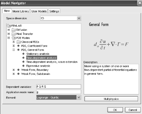
In figure (1) we start selecting the dimensionality of the problem (1D), the type of problem (time dependent in general form), the variables $(P,Q,R,S)$ and the element (Lagrange quintic). We adopted the highest nonlinear element in order to get the best results, although a quadratic Lagrange element leads practically the same results (with smaller computational time).

Figure 1: Choosing the model properties.

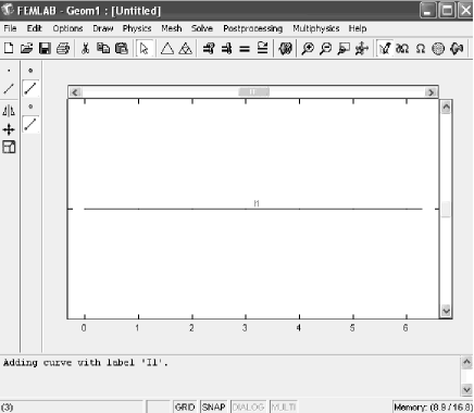
In figure (2) we draw the domain, i.e. a line starting at $x=0$ and ending at $x=2\pi$.

Figure 2: Drawing the spatial domain.

In figures (3)-(5) we insert the field equations in divergence form while in figure (6) we enter the initial data.

Figure 3: Entering field equations (first part).

Figure 4: Entering field equations (second part).

Figure 5: Entering field equations (third part).

Figure 6: Entering initial data.

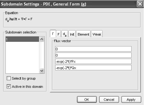
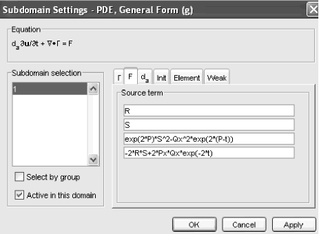
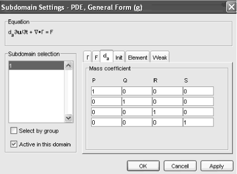
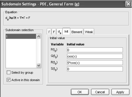
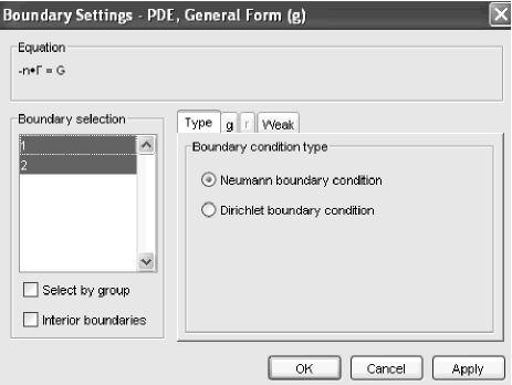
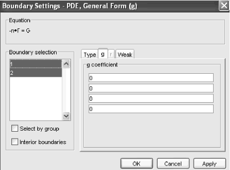
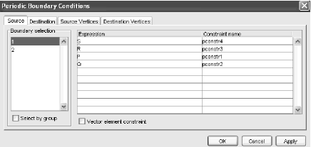
In these FEMLAB modeling pictures as well as in the forthcoming text and figures, time $t$ has always to be intended as scaled time $\tau$ of equations (2). In figures (7) and (8) instead we chose zero flux Neumann boundary conditions at both ends of the domain, while in figure (9) one enters the periodic boundary conditions (which as described before, are automatically implied by zero flux ones). We show one figure only because the entire procedure would take several slides due to the fact that one has to make the value of the various field coincide at both ends (vertices). The procedure is very simple, although takes few minutes and is well explained in the online manual with several examples so we refer to it for this part of the model.

Figure 7: Selecting zero flux conditions (first part).

Figure 8: Selecting zero flux conditions (second part).

Figure 9: Selecting periodic boundary conditions (see text).

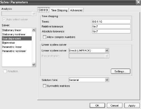
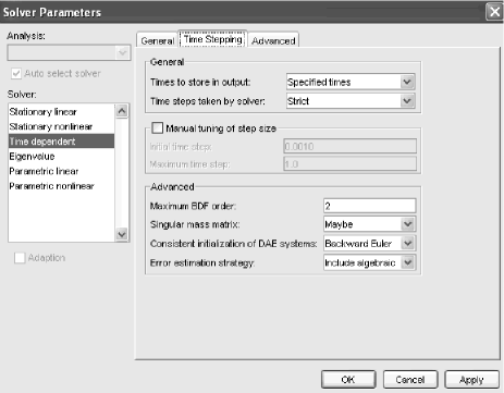
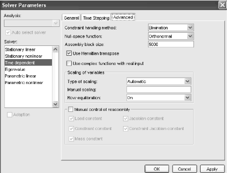
In figures (10)-(12) we select the numerics of the problem. A direct solver (UMFPACK) is chosen, time integration starts at $t=0$ and ends at $t=10$, saving on hard disk the simulation results at every $0.1$ time step. Other options are chosen in order to have the most precise settings for the simulation. Time stepping is automatically chosen by the solver which refines it when necessary (although one can always set it up manually). Concerning numerical accuracy, we have selected relative and absolute tolerance thresholds of $10^{-7}$. This choice will be sufficient to get high quality results.

Figure 10: Selecting numeric properties (first part).

Figure 11: Selecting numeric properties (second part).

Figure 12: Selecting numeric properties (third part).

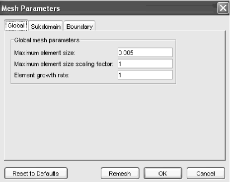
In figure (13) we select the meshing of the domain, which is uniform and has a spacing of $\Delta x=0.005$. While FEMLAB can handle adaptive mesh refinement, we prefer to use such a very fine constantly spaced meshing here.

Figure 13: Selecting meshing properties.

IV Results

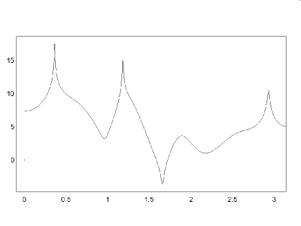
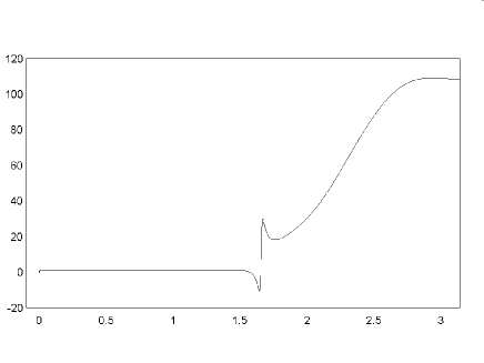
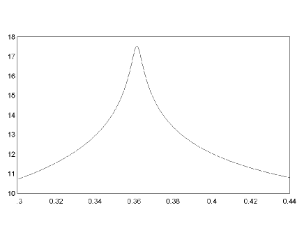
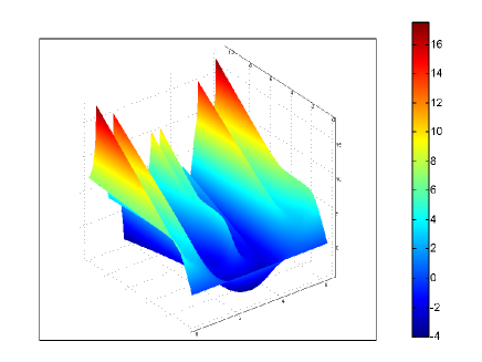
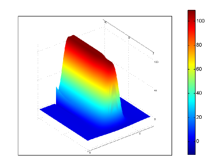
As anticipated before, simulation takes approximately ten minutes to run on a Pentium $4$ running at $1.7$GHz. In figure (14) we show $P$ at $t=10$, in the interval $0\leq x\leq\pi$, while figure (15) is a plot of $Q$ with same conditions. Figure (16) shows a detail (a spike) of figure (14). These three figures are exactly coincident with figures $1,2$, and $3$ of reference Garfinkle , i.e. FEMLAB produced the same results of finite differences simulations using finite elements instead. In figures (17) and (18) we show the time evolution in the entire spatial domain of $P$ and $Q$ respectively. This visualization clearly shows the generation and subsequent development of these Gowdy spikes. The initial data for $Q$, i.e. $\cos x$ is not evident in figure (18) due to the very large change of scale, which has passed from $1$ to around $100$ in ten time units.

Figure 14: Plot of $P$ at $t=10$ (read $\tau$) for $0\leq x\leq\pi$.

Figure 15: Plot of $Q$ at $t=10$ (read $\tau$) for $0\leq x\leq\pi$.

Figure 16: Detail of the plot for $P$ at $t=10$ (read $\tau$) around $x=0.36$.

Figure 17: Time evolution of $P$ in the interval $0\leq x\leq 2\pi$.

Figure 18: Time evolution of $Q$ in the interval $0\leq x\leq 2\pi$.

V Discussion

The simulation presented in this article and the comparison with existing literature suggests that FEMLAB can become for sure a necessary tool for those scientists and mathematicians working in the field of GR analysis, as in the past years Maple with its tensor packages did. Due to its possibility to handle general PDEs, problems in astrophysics (equilibrium configurations, MHD, …) and in more general theories of gravitation like EMDA and branes can be solved. Being FEMLAB totally integrated in MATLAB, and having MAPLE a direct export to it, the process of symbolic derivation of field equation, numerical solution and export for deeper analysis ( for studying the solution in the frequency domain in order to extract quasi-normal modes, for example) and comparison with experimental data results straightforward. Moreover, being FEMLAB designed for $64$bit platforms, large amounts of memory (typically a ten of Gb) can be addressed for simulations in 2D and 3D, although for the latter case, having in mind General Relativity problems like strongly distorted black holes and neutron stars, a parallelized version of the software would certainly be welcome. Even for those working in Numerical Relativity, the use of FEMLAB allows them to test an idea in a simplified version in few hours, and if the obtained results appear to be promising, write down then an optimized code for their large scale supercomputers.

VI Acknowledgments

CC would like to thank the organizers of the 9th Italian-Korean Symposium on Relativistic Astrophysics, and Prof H.W. Lee in particular, for their continuous and efficient assistance during the entire conference in Korea. All trademarks and registered trademarks are the property of their respective owners.

References

- (1) C. Cherubini, F. Federici, S. Succi and M. P. Tosi, ”Excised acoustic black holes: the scattering problem in the time domain”, preprint gr-qc/0504048 (2005).
- (2) F. Federici, C. Cherubini, S. Succi and M. P. Tosi, ”Superradiance from BEC vortices: a numerical study”, preprint gr-qc/0503089 (2005).
- (3) M.A. Scheel, A.L. Erickcek, L.M. Burko, L.E. Kidder, H.P. Pfeiffer and S.A. Teukolsky , Physical Review D, 69, 104006 (2004).
- (4) D. Garfinkle , Class. Quant. Grav. , 21, 219 (2004); preprint gr-qc/0408018 v1.
- (5) T.J.R. Hughes The Finite Element Method: Linear Static and Dynamic Finite Element Analysis , Dover Publications, (2000).