Stockholm
USITP 05-4
September 2005
Revised November 2005

We study the Lorentzian analogues of the squashed 3-sphere, namely 2+1 dimensional anti-de Sitter space squashed or stretched along fibres that are either spacelike or timelike. The causal structure, and the property of being an Einstein–Weyl space, depend critically on whether we squash or stretch. We argue that squashing, and stretching, completely destroys the conformal boundary of the unsquashed spacetime. As a physical application we observe that the near horizon geometry of the extremal Kerr black hole, at constant Boyer–Lindquist latitude, is anti-de Sitter space squashed along compactified spacelike fibres.

1. Introduction

The Hopf fibration of the 3-sphere appears throughout mathematical physics in many guises; it is used to describe qubits, magnetic monopoles, Taub-NUT universes, and what not. There is a beautiful picture behind it: the Hopf fibres form a space-filling congruence of linked geodesic circles in the 3-sphere. In the Taub-NUT cosmologies the 3-sphere is squashed along the Hopf fibres. Such spheres are known as Berger spheres by mathematicians. They are solutions to the conformally invariant Einstein–Weyl equations.

The squashed 3-sphere has a Lorentzian analogue. In fact it has two Lorentzian analogues, since 3 dimensional anti-de Sitter space ${\bf adS}_{3}$ can be squashed (or stretched) along Hopf fibres that are either spacelike or timelike. This construction was briefly discussed by Jones, Tod and Pedersen [1] [2], because such spacetimes admit a twistorial description (with a two dimensional family of totally geodesic null hypersurfaces serving as twistor space [3]). From this point of view squashed anti-de Sitter space becomes interesting as a simple but non-trivial example in twistor theory. It has also been studied as an asymmetric deformation of the conformal field theory that describes the propagation of strings on the group manifold of $SL(2,{\bf R})$—also known as ${\bf adS}_{3}$ [4, 5]. But there are other uses of such a natural construction, in particular the near horizon geometry of the extremal Kerr black hole [6] can be understood using it. For this reason we have studied squashed anti-de Sitter space in some detail. We also use it to point a moral: we will argue that the squashing completely destroys the conformal boundary of the unsquashed spacetime. This tells us that conformal compactification [7] depends much more on the detailed structure of Einstein’s equations than one might perhaps think it would.

The contents of this paper: We describe some relevant features of 2+1 dimensional anti-de Sitter space in section 2, but since this has been described at length elsewhere—we recommend ref. [8] and references therein—some details are relegated to an Appendix. In section 2 we concentrate on the two geodetic congruences, one timelike and one spacelike, that will play the role that the Hopf circles play for the 3-sphere. In section 3 we squash and stretch our spacetime along these fibres, discuss the symmetries of the resulting spacetimes, and find the Killing horizons that they contain. Section 4 makes some observations on null geodesics; the distinction between squashing and stretching now begins to become apparent. For timelike stretching detailed results are available already—we are in effect studying the Gödel spacetime [9]. In section 5 we establish when our spacetimes solve the conformally invariant Einstein–Weyl equations. In section 6 we attempt to conformally compactify our spacetimes, and argue that the boundary is destroyed by squashing (and stretching). Section 7 applies what we have learned to a discussion of the extremal Kerr black hole. Conclusions and open questions are briefly listed in section 8.

2. Geodetic congruences in anti-de Sitter space

Anti-de Sitter space is defined as a quadric surface embedded in a flat space of signature $(+\dots+--)$. Thus 2+1 dimensional anti-de Sitter space is defined as the hypersurface

$$X^{2}+Y^{2}-U^{2}-V^{2}=-1$$ (1)

embedded in a 4 dimensional flat space with the metric

$$ds^{2}=dX^{2}+dY^{2}-dU^{2}-dV^{2}\ .$$ (2)

The Killing vectors are denoted $J_{XY}=X\partial_{Y}-Y\partial_{X}$, $J_{XU}=X\partial_{U}+U\partial_{X}$, and so on. The topology is now ${\bf R}^{2}\times{\bf S}^{1}$, and one may wish to go to the covering space in order to remove the closed timelike curves. Our arguments will mostly not depend on whether this final step is taken.

For the 2+1 dimensional case the definition can be reformulated in an interesting way. Anti-de Sitter space can be regarded as the group manifold of $SL(2,{\bf R})$, that is as the set of matrices

$$g=\left[\begin{array}[]{cc}V+X&Y+U\\ Y-U&V-X\end{array}\right]\ ,\hskip 28.45274pt\mbox{det}g=U^{2}+V^{2}-X^{2}-Y^{2}=1\ .$$ (3)

The group manifold is equipped with its natural metric, which is invariant under transformations $g\rightarrow g_{1}gg_{2}^{-1}$, $g_{1},g_{2}\in SL(2,{\bf R})$. The Killing vectors can now be organized into two orthonormal and mutually commuting sets,

$$J_{1}=-J_{XU}-J_{YV}\hskip 42.67912pt \tilde{J}_{1}=-J_{XU}+J_{YV}$$ (4)

$$J_{2}=-J_{XV}+J_{YU}\hskip 42.67912pt \tilde{J}_{2}=-J_{XV}-J_{YU}$$ (5)

$$J_{0}=-J_{XY}-J_{UV}\hskip 42.67912pt \tilde{J}_{0}=J_{XY}-J_{UV}\ .$$ (6)

They obey

$$||J_{1}||^{2}=||J_{2}||^{2}=-||J_{0}||^{2}=1\ ,\hskip 8.53581pt||\tilde{J}_{1}||^{2}=||\tilde{J}_{2}||^{2}=-||\tilde{J}_{0}||^{2}=1\ .$$ (7)

Locally $SL(2,{\bf R})$ is isomorphic with the Lorentz group $SO(2,1)$. The isometry group $SO(2,2)$ is therefore locally isomorphic to $SO(2,1)\times SO(2,1)$. These matters are discussed more fully in ref. [8]. Very similar things can be said about the 3-sphere.

Here we would like to describe a coordinate system $(\tau,\omega,\sigma)$ [10], analogous to the Euler angles that are used to describe the 3-sphere. To this end we parametrize an arbitrary $SL(2,{\bf R})$ matrix as

$$g(\tau,\omega,\sigma)=\left[\begin{array}[]{cc}\cos{\frac{\tau}{2}}&-\sin{\frac{\tau}{2}}\\ \sin{\frac{\tau}{2}}&\cos{\frac{\tau}{2}}\end{array}\right]\left[\begin{array}[]{cc}\sinh{\frac{\omega}{2}}&\cosh{\frac{\omega}{2}}\\ -\cosh{\frac{\omega}{2}}&-\sinh{\frac{\omega}{2}}\end{array}\right]\left[\begin{array}[]{cc}\exp{-\frac{\sigma}{2}}&0\\ 0&\exp{\frac{\sigma}{2}}\end{array}\right]\ .$$ (8)

Straightforward calculations show that the Killing vectors in the first $SO(2,1)$ factor are

$$J_{1} = -\frac{2\sinh{\sigma}}{\cosh{\omega}}\partial_{\tau}-2\cosh{\sigma}\partial_{\omega}+2\tanh{\omega}\sinh{\sigma}\partial_{\sigma}$$ (9)

$$J_{2} = 2\partial_{\sigma}$$ (10)

$$J_{0} = \frac{2\cosh{\sigma}}{\cosh{\omega}}\partial_{\tau}+2\sinh{\sigma}\partial_{\omega}-2\tanh{\omega}\cosh{\sigma}\partial_{\sigma}\ .$$ (11)

The second $SO(2,1)$ factor is spanned by

$$\tilde{J}_{1} = 2\sin{\tau}\tanh{\omega}\partial_{\tau}-2\cos{\tau}\partial_{\omega}+\frac{2\sin{\tau}}{\cosh{\omega}}\partial_{\sigma}$$ (12)

$$\tilde{J}_{2} = -2\cos{\tau}\tanh{\omega}\partial_{\tau}-2\sin{\tau}\partial_{\omega}-\frac{2\cos{\tau}}{\cosh{\omega}}\partial_{\sigma}$$ (13)

$$\tilde{J}_{0} = 2\partial_{\tau}\ .$$ (14)

We will focus on the mutually commuting Killing vectors $J_{2}$ and $\tilde{J}_{0}$, to which our coordinate system is adapted. They form two nowhere vanishing vector fields in ${\bf adS}_{3}$. In any odd dimensional anti-de Sitter space we can construct a nowhere vanishing timelike vector field analogous to $\tilde{J}_{0}$, while there is no similar higher dimensional analogue for $J_{2}$. But in dimension 3 we have these two everywhere vanishing vector fields to play with. Each of them defines an interesting congruence in anti-de Sitter space, and their flow lines are the Hopf fibres along which we will squash and stretch our spacetime.

The metric on anti-de Sitter space takes the form

$$ds^{2} = \frac{1}{4}(-d\tau^{2}+d\omega^{2}+d\sigma^{2}+2\sinh{\omega}d\tau d\sigma)=$$ (15)

(16)

$$= \frac{1}{4}\left(-(d\tau-\sinh{\omega}d\sigma)^{2}+d\omega^{2}+\cosh^{2}{\omega}d\sigma^{2}\right)$$

(17)

$$= \frac{1}{4}\left(-\cosh^{2}{\omega}d\tau^{2}+d\omega^{2}+(d\sigma+\sinh{\omega}d\tau)^{2}\right)\ .$$

The flow lines of our two Killing vector fields are geodesics, so we are dealing with two geodetic congruences.

We will soon draw pictures of these congruences. To do so it is convenient to use another coordinate system, namely the sausage coordinates described in the Appendix. Then anti-de Sitter space itself will appear as a cylinder sliced with Poincaré disks of constant negative curvature.

One more remark about the symmetries of anti-de Sitter space is needed. (We make it brief, because it was fully spelt out elsewhere [8, 11].) We will be especially interested in the Killing horizons that arise. For what conjugacy classes of isometries does this happen? To answer this question one begins with the observation that the conjugacy classes of $SO(2,1)$ can be divided into hyperbolic, elliptic and parabolic transformations. Since the group manifold of $SO(2,1)$, or more precisely its double covering $SL(2,{\bf R})$, is itself a copy of ${\bf adS}_{3}$, these conjugacy classes correspond to two dimensional surfaces in the group manifold (with the parabolic conjugacy classes forming the forwards and backwards lightcones of the origin). Since the Lie algebra of $SO(2,2)$ is a direct product of two copies of the Lie algebra of $SO(2,1)$, it is then straightforward to divide the Killing vectors of the former group into conjugacy classes. Further, it is known that bifurcate Killing horizons in ${\bf adS}_{3}$ occur for conjugacy classes where the transformations take the form (hyperbolic) $\times$ (hyperbolic); they are numerous enough so that every spacelike geodesic is the bifurcation line of such a Killing horizon. Degenerate Killing horizons occur for transformations of the form (parabolic) $\times$ (parabolic). They form a two parameter family of totally geodesic null surfaces, and can be regarded as light cones with vertices on the conformal boundary . Finally transformations of the type (parabolic) $\times$ (identity) have Killing vector fields that are everywhere null.

To understand the Hopf fibration of the 3-sphere, it is helpful to begin with the observation that every Hopf circle lies on one of a space filling set of tori—indeed on a set of intrinsically flat tori of varying size and shape [12]. We will now study our congruences in the same spirit, beginning with the timelike geodetic congruence generated by $\tilde{J}_{0}$ and coinciding with the $\tau$ coordinate lines. All the geodesics in the $\tilde{J}_{0}$ congruence are timelike and lie on a set of intrinsically flat Lorentzian tori, defined by

$$X^{2}+Y^{2}=\mbox{constant}\ .$$ (18)

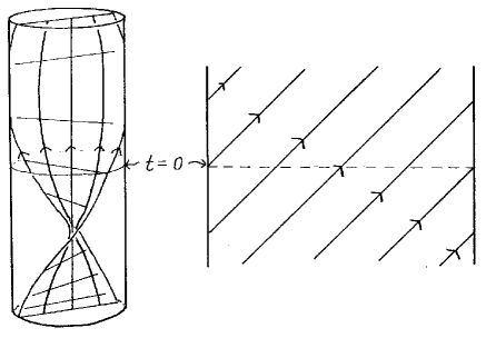
Figure 1: This picture is drawn using the sausage coordinates from the Appendix. It shows anti-de Sitter space as a cylinder (with a conformal boundary). The timelike congruence consists of timelike spirals ruling a set of helicoids. To the right we show that the flow becomes null on the boundary.

These are tori because (or if) anti-de Sitter space is periodic in the time direction. Surfaces of constant $\sigma$ are also ruled by these geodesics. In particular the surface

$$XV-VY=0\hskip 14.22636pt\Leftrightarrow\hskip 14.22636pt\sigma=0$$ (19)

is flat and minimal. We draw it in Fig. 1, using the sausage coordinates from the Appendix. In sausage coordinates the Killing vector becomes $\tilde{J}_{0}=\partial_{t}+\partial_{\phi}$, the congruence consists a set of helices, and the surface $\sigma=0$ is known as the helicoid. (It is a minimal surface in coordinate space too.) Note that the geodesics become null on the conformal boundary . There are no fixed points anywhere.

The spacelike congruence, generated by $J_{2}$ and coinciding with the $\sigma$ coordinate lines, is harder to draw. The first observation is that also these geodesics become null on , although in this case there are two lines of fixed points; there are sources at $t-\phi=\pi/2$ and sinks at $t-\phi=-\pi/2$. Inside anti-de Sitter space the congruence is everywhere spacelike, and every Poincaré disk defined by $t=$ constant contains one member of the congruence. Surfaces of constant $\tau$, which are flat and minimal, are ruled by these geodesics but are rather hard to draw. Another surface that is ruled by these geodesics is the totally geodesic null surface

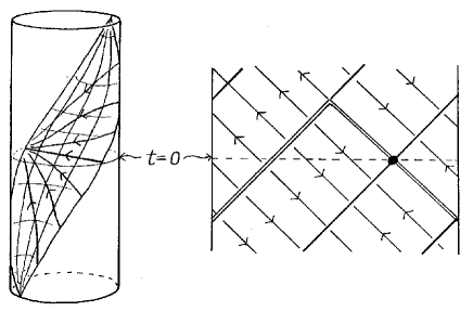
Figure 2: Again using sausage coordinates we show the null surface $X=V$, and how it is ruled by the spacelike congruence. To the right we show that the flow becomes null on the boundary, and where it has fixed points. There is a special point acting as a sink for all those members of the congruence that belong to the null surface shown.

$$X=V\ .$$ (20)

In fact this surface contains every $J_{2}$ geodesic that goes to a particular sink on , and is fairly easy to draw (Fig. 2). The one parameter family of null surfaces

$$X\cos{\beta}+Y\sin{\beta}+U\sin{\beta}-V\cos{\beta}=0$$ (21)

provides a foliation of anti-de Sitter space with null surfaces ruled by the $J_{2}$ geodesics. Moreover this very family of null surfaces will be of importance for our discussion of squashed anti-de Sitter space later on.

We can already see that trouble is brewing on  once we decide to squash our spacetime along these fibres (keeping all distances orthogonal to the fibres constant). On the boundary the fibres are changing character, from timelike/spacelike to null. Therefore squashing  is a different matter than squashing the interior. Moreover, we expect—and this is true—that the result of squashing all the way down to zero distance along the spacelike fibres will result in a two dimensional anti-de Sitter space. But this spacetime has a  consisting of two disconnected components. Somewhere along the way, something has to break.

3. Squashing, stretching, and symmetries

It is time to introduce the spacetime analogues of the Berger sphere. We obtain them by squashing ${\bf adS}_{3}$ along one of the two congruences described in the previous section. The resulting spacetimes will be homogeneous but anisotropic, and we will study their symmetries in some detail.

Let us consider the spacelike case first; it has some special features that, in the end, make this case the easiest to understand—especially if Fig. 2 is kept firmly in mind. The metric on squashed ${\bf adS}_{3}$ is

$$ds^{2}_{\lambda}=\frac{1}{4}\left(-\cosh^{2}{\omega}d\tau^{2}+d\omega^{2}+\lambda^{2}(d\sigma+\sinh{\omega}d\tau)^{2}\right)\ ,$$ (22)

where $\lambda$ is a real squashing parameter. If we set it to zero we obtain the metric on ${\bf adS}_{2}$ in a well known coordinate system—which is the familiar fact that ${\bf adS}_{3}/{\bf R}={\bf adS}_{2}$, analogous to the fact that ${\bf S}^{3}/{\bf S}^{1}={\bf S}^{2}$. Note however that—unlike its analogue for the 3-sphere—this particular result does not have any straightforward higher dimensional analogue.

Because of the squashing the isometry group is now four dimensional. The Lie algebra changes from $SO(2,1)\times SO(2,1)$ for the unsquashed spacetime to $R\times SO(2,1)$ for the squashed one; the left factor here gives transformations belonging to a hyperbolic conjugacy class of $SO(2,1)$. The question we ask is whether any Killing horizons survive. The answer is yes. There will be bifurcate Killing horizons coming from transformations of the type (hyperbolic) $\times$ (hyperbolic), although they will be less numerous than they were in anti-de Sitter space. The degenerate Killing horizons that were present in the unsquashed case are no longer with us, since they came from transformations of the type (parabolic) $\times$ (parabolic). But there were also totally null Killing vector fields in anti-de Sitter space, coming from transformations of the type (identity) $\times$ (parabolic). Once we have done the squashing this will give us a supply of degenerate Killing horizons, as a replacement for those that were lost.

But we do not have to rely on any previous results here. A short calculation verifies that the most general Killing vector field that has a spacelike curve of fixed points is (up to scale)

$$\xi=J_{2}+a\tilde{J}_{1}+b\tilde{J}_{2}+c\tilde{J}_{0}\ ,$$ (23)

where the real numbers $a$, $b$, $c$ obey

$$a^{2}+b^{2}-c^{2}=1\ .$$ (24)

This is a timelike surface in the group manifold of $SO(2,1)$. The fixed points occur at

$$\sinh{\omega}=c\ ,\hskip 17.07164pt\cos{\tau}=\frac{b}{\sqrt{a^{2}+b^{2}}}\hskip 11.38109pt\sin{\tau}=-\frac{a}{\sqrt{a^{2}+b^{2}}}\ .$$ (25)

These curves are precisely the fibres along which we are squashing. They are also bifurcation curves for bifurcate Killing horizons. Hence squashed anti-de Sitter space contains a two parameter family of bifurcate Killing horizons. The unsquashed spacetime has more: in anti-de Sitter space itself every spacelike geodesic is a bifurcation line for some Killing horizon.

If we pick an example in this class, we find that

$$||J_{2}+\tilde{J}_{2}||^{2}=(1-\cos{\tau}\cosh{\omega})\left(\lambda^{2}+1-(\lambda^{2}-1)\cos{\tau}\cosh{\omega}\right)\ .$$ (26)

The surface gravity $\kappa$ is given by $|\kappa|=2$. A feature that arises only in the squashed case is that there are actually two surfaces where the norm vanishes, but only one of them is a Killing horizon—the other is a timelike surface.

A one parameter family of degenerate Killing horizons arise from the Killing vectors

$$\tilde{\xi}(\alpha)=\cos{\alpha}\tilde{J}_{1}+\sin{\alpha}\tilde{J}_{2}+\tilde{J}_{0}\ .$$ (27)

This time the norm is

$$||\tilde{\xi}(\alpha)||^{2}=(\lambda^{2}-1)(\sinh{\omega}+\sin{(\tau-\alpha)}\cosh{\omega})^{2}\ .$$ (28)

In ${\bf adS}_{3}$ these Killing vectors are everywhere null. In the squashed case ($\lambda^{2}<1$) they are timelike except for a degenerate Killing horizon where the norm vanishes, and in the stretched case ($\lambda^{2}>1$) they are spacelike again except for a degenerate Killing horizon. In anti-de Sitter space itself this family of null surfaces is identical to the family given in eq. (21), if we set $\alpha=2\beta+\pi$. In the anti-de Sitter case there are additional degenerate Killing horizons that disappear when we squash or stretch.

Since we are primarily interested in Killing horizons because they are totally geodesic null surfaces, it is enough to consider degenerate horizons—the bifurcate ones do not contribute anything new in this way.

Next we squash or stretch along the timelike congruence. Then the metric is

$$ds_{\lambda}^{2}=\frac{1}{4}\left(-\lambda^{2}(d\tau-\sinh{\omega}d\sigma)^{2}+d\omega^{2}+\cosh^{2}{\omega}d\sigma^{2}\right)\ .$$ (29)

Setting $\lambda=0$ results in the metric on the hyperbolic plane, expressing the well known fact that ${\bf adS}_{3}/{\bf S}^{1}={\bf H}^{2}$. In general the symmetry group is $SO(2)\times SO(2,1)$. This means that there are no bifurcate Killing horizons anymore. There are no degenerate horizons either. We may try

$$\xi=J_{2}+J_{0}\ ,$$ (30)

which is everywhere null in anti-de Sitter space. After (timelike) squashing we obtain

$$||\xi||^{2}=-(\lambda^{2}-1)(\cosh{\omega}\cosh{\sigma}-\sinh{\omega})^{2}\ .$$ (31)

This is timelike or spacelike, depending on whether we squash or stretch.

4. Null geodesics

Our spacetimes have enough symmetries to ensure that the geodesic equation can be separated. It is particularly interesting to take a look at the equations for null geodesics, because there is a surprise waiting. We will discuss the case of spacelike squashing in some detail, and comment briefly on timelike squashing at the end. For a related discussion, including some interesting observations on timelike geodesics, see Bardeen and Horowitz [6].

We begin by introducing the convenient coordinate

$${\rm w}=\sinh{\omega}\ .$$ (32)

Using it, it is straightforward to bring the equations for a null geodesic with respect to the metric (22) to the form

$$\dot{\tau}=\frac{1+\lambda{\rm w}\sin{\phi}}{1+{\rm w}^{2}}$$ (33)

$$\dot{\sigma}=\frac{\sin{\phi}}{\lambda}-\frac{\rm w}{1+{\rm w}^{2}}(1+\lambda{\rm w}\sin{\phi})$$ (34)

$$\dot{\rm w}^{2}=\cos^{2}{\phi}+2\lambda{\rm w}\sin{\phi}+(\lambda^{2}-1){\rm w}^{2}\sin^{2}{\phi}\ .$$ (35)

Without loss of generality we have chosen the integration constants to ensure that the geodesic passes the origin of our coordinate system. The first observation is that if $\sin{\phi}=0$ then $\lambda$ drops out of the equations; this corresponds to a null geodesic that is everywhere orthogonal to the squashing direction. Such geodesics are unaffected by any squashing (or stretching). This is actually true also for spacelike and timelike geodesics orthogonal to the squashing direction, as well as for the spacelike geodesics that are parallel to this direction. Note also that we have come across null geodesics orthogonal to the squashing direction once before—they rule the Killing horizons depicted in Fig. 2.

Let us now assume that $\sin{\phi}\neq 0$. Asymptotically, that is to say for large values of ${\rm w}$, we obtain

$$\dot{\tau}\sim\frac{\lambda\sin{\phi}}{\rm w}$$ (36)

$$\dot{\sigma}\sim(1-\lambda^{2})\frac{\sin{\phi}}{\lambda}$$ (37)

$$\dot{\rm w}^{2}\sim(\lambda^{2}-1){\rm w}^{2}\sin^{2}{\phi}\ .$$ (38)

Evidently it is possible to reach arbitrarily large values of ${\rm w}$ only if $\lambda^{2}\geq 1$, that is to say only for stretching, not for squashing. This is the surprise that we were referring to.

The explicit solution for ${\rm w}(s)$ can be written down, but is not very illuminating—we get the expected oscillatory behaviour for squashing, while stretching gives an exponentially growing function. To go on, when $\lambda^{2}>1$ we see that

$${\rm w}\rightarrow\infty\hskip 14.22636pt\Rightarrow\hskip 14.22636pt\sigma\rightarrow\pm\infty\ .$$ (39)

This is a very different kind of behaviour from that occurring in the unstretched anti-de Sitter case. In effect, asymptotically the null geodesics are lining up with the null geodesics that rule the Killing horizons described in the previous section. The implications of this will be discussed in section 6.

For the case of timelike squashing fibres detailed results are available in the literature already. This is because, by adding an extra flat direction, and specializing the stretching parameter to $\lambda^{2}=2$ [9], the resulting 3+1 dimensional spacetime is the famous Gödel solution. An elegant review of its null geodesics has been given by Ostváth and Schucking [13]; to follow them we use the coordinate system given just before eq. (91) in the Appendix, and perform the further coordinate changes

$$T=\frac{1}{2}(\psi-\phi)\ ,\hskip 17.07164pt\cosh{\theta}=\frac{1+R^{2}}{1-R^{2}}\ ,\hskip 8.53581pt\sinh{\theta}=\frac{2R}{1-R^{2}}\ ,\hskip 8.53581pt0<R<1\ .$$ (40)

This brings the metric to the form

$$ds^{2}=\frac{1}{(1-R^{2})^{2}}\left[-\lambda^{2}\left((1-R^{2})dT-R^{2}d\phi\right)^{2}+dR^{2}+R^{2}d\phi^{2}\right]\ .$$ (41)

When we study null geodesic paths we may ignore the conformal factor in front of the metric. What one finds [13] is that a null geodesic through the origin of our coordinate system obeys

$$R=\frac{1}{\lambda}\sin{(\phi+\phi_{0})}\ .$$ (42)

Setting $\phi_{0}=0$ and trading $R$ and $\phi$ for Cartesian coordinates on the Poincaré disk gives

$$\sqrt{x^{2}+y^{2}}=\frac{1}{\lambda}\frac{y}{\sqrt{x^{2}+y^{2}}}\hskip 14.22636pt\Leftrightarrow\hskip 14.22636ptx^{2}+\left(y-\frac{1}{2\lambda}\right)^{2}=\left(\frac{1}{2\lambda}\right)^{2}\ .$$ (43)

This is a circle. The family of null geodesics through the origin, projected down to the Poincaré disk, are circles whose envelope is a circle with radius $1/\lambda$.

Thus when $\lambda^{2}>1$ all null geodesics are confined to the interior of stretched anti-de Sitter space. When $R=1$ the conformal factor in front of the metric diverges, so that what happens when $\lambda=1$ is that the null geodesics touch  but they slow down there in such a way that there is no turning back. In the squashed case ($\lambda^{2}<1$) the null geodesics escape. Detailed examination shows that the squashed case differs from the anti-de Sitter case in that the null geodesics reach arbitrarily large values of the coordinate $T$, rather than end up at a finite value of $T$ as they do in anti-de Sitter space.

We may further observe that

$$||\partial_{\phi}||^{2}=\frac{R^{2}}{(1-R^{2})^{2}}(1-\lambda^{2}R^{2})\ .$$ (44)

Hence $\lambda^{2}>1$ implies that there are closed timelike curves beyond the envelope of the null geodesics; this, of course, was one of Gödel’s main points. In the squashed case no such thing happens. Indeed

$$dT^{2}=0\hskip 14.22636pt\Rightarrow\hskip 14.22636ptds^{2}=\frac{1}{(1-R^{2})^{2}}\left(dR^{2}+R^{2}(1-\lambda^{2}R^{2})d\phi^{2}\right)\ .$$ (45)

Thus when $\lambda^{2}<1$ the coordinate $T$ serves as a global time function, and there can be no CTCs, unless this direction is compactified. There are no CTCs in the case of spacelike squashing or stretching either.

In the next section we will observe another key difference between squashing and stretching, and between spacelike and timelike fibres.

5. The Einstein–Weyl equations

The Einstein–Weyl equations are a conformally invariant set of equations involving a metric tensor and a vector potential. They were introduced by Weyl in an attempt to unify gravitation and electromagnetism [14]; his theory failed but left a valuable legacy. We will give the basic facts only; for a more complete summary see Pedersen and Tod [2].

By definition, a Weyl space is a manifold equipped by a metric $g_{ab}$, a one-form $\omega_{a}$, and a connection—known as the Weyl connection—which are compatible in the sense that

$$D_{a}g_{bc}=\omega_{a}g_{bc}\ .$$ (46)

The solution is

$$D_{a}V^{b}=\nabla_{a}V^{b}+{\gamma}^{b}_{\ ac}V^{c}$$ (47)

where $\nabla_{a}$ is defined by the usual metric compatible Levi-Civita connection and

$${\gamma}^{b}_{\ ac}=-\frac{1}{2}(\delta^{b}_{a}\omega_{c}+\delta^{b}_{c}\omega_{a}-g_{ac}g^{bd}\omega_{d})\ .$$ (48)

Given a Weyl space, the pair $(g^{\prime}_{ab},\omega^{\prime}_{c})=(e^{\Omega}g_{ab},\omega_{c}+\partial_{c}{\Omega})$ defines a Weyl space too.

The Weyl connection has a curvature tensor defined by

$$[D_{a},D_{b}]V_{c}=W_{abc}^{\ \ \ d}V_{d}\ .$$ (49)

We also define

$$W_{ab}=W_{acb}^{\ \ \ c}\hskip 14.22636pt\mbox{and}\hskip 14.22636ptW=g^{ab}W_{ab}\ .$$ (50)

Note that $W_{ab}$ is not symmetric in general. A calculation shows that

$$W_{(ab)} = R_{ab}+\frac{1}{2}\nabla_{(a}\omega_{b)}+\frac{1}{4}\omega_{a}\omega_{b}+g_{ab}\left(\frac{1}{2}\nabla_{c}\omega^{c}-\frac{1}{4}\omega^{2}\right)$$ (51)

$$W_{[ab]} = \frac{3}{2}\nabla_{[a}\omega_{b]}\equiv\frac{3}{2}F_{ab}\ ,$$ (52)

where square and round brackets denote anti-symmetrization and symmetrization, respectively. Notice the definition of $F_{ab}$. It is easy to see that

$$W_{ab}^{\ \ cd}=W_{ab}^{\ \ [cd]}+F_{ab}g^{cd}\ ,$$ (53)

and moreover—because we are in 3 dimensions—

$$W_{ab}^{\ \ cd}=\epsilon_{abe}\epsilon^{cdf}\left(\frac{1}{2}\delta_{f}^{e}W-W_{f}^{\ e}-F_{f}^{\ e}\right)\ .$$ (54)

By definition a three dimensional Einstein–Weyl space obeys

$$W_{(ab)}=\frac{1}{3}Wg_{ab}\ .$$ (55)

For the ordinary Ricci tensor this implies that

$$R_{ab}+\frac{1}{2}\nabla_{(a}\omega_{b)}+\frac{1}{4}\omega_{a}\omega_{b}=g_{ab}\left(\frac{1}{3}W-\frac{1}{2}\nabla_{c}\omega^{c}+\frac{1}{4}\omega^{2}\right)=\Lambda g_{ab}\ ,$$ (56)

where $\Lambda$ is some function. In the Einstein case the Bianchi identities force $\Lambda$ to equal a constant, but this is no longer true here. Unlike the Einstein equations, the Einstein–Weyl equations admit an infinitude of locally inequivalent solutions in 3 dimensions. It was shown by Cartan that these solutions can be specified by four arbitrary functions of two variables [15].

Does squashed anti-de Sitter space obey the Einstein–Weyl equations? For the spacelike case, we start with the metric (22) and compute the Ricci tensor. We must then find a one-form $\omega_{a}$ such that eq. (56) holds for some $\Lambda$. What we actually find is that

$$R_{ab}+\lambda^{2}(\lambda^{2}-1)\xi_{a}\xi_{b}=2(\lambda^{2}-2)g_{ab}\ ,$$ (57)

where the one-form $\xi^{a}$ is the Killing vector field that defines the squashing,

$$\xi_{a}=\nabla_{a}\sigma+\sinh{\omega}\nabla_{a}\tau\ \hskip 14.22636pt\Rightarrow\hskip 14.22636pt\nabla_{(a}\xi_{b)}=0\ .$$ (58)

Therefore we obtain a solution of the Einstein–Weyl equation if we perform the rescaling

$$\frac{1}{2}\omega_{a}\equiv\sqrt{\lambda^{2}(\lambda^{2}-1)}\xi_{a}\ .$$ (59)

Curiously a real solution is obtained only for $\lambda^{2}\geq 1$, that is to say if we stretch anti-de Sitter space, but not if we squash it. For timelike squashing, we obtain a real solution when we squash but not when we stretch; this is also true for the Riemannian Berger sphere [2]. We do not fully understand why this should be so. We observe that, in anti-de Sitter space, spacelike geodesics tend to diverge, and timelike geodesics tend to converge. Geodesics on the 3-sphere tend to converge as well. Perhaps more to the point, in the previous section we noted that null geodesics behave very differently depending on whether the spacetime is squashed or streched.

With the Weyl connection in hand we can define a new notion of geodesic curves. We will continue to refer to geodesics with respect to our chosen metrics as “geodesics”, while geodesics with respect to the Weyl connection will be called “Weyl geodesics”. Cartan proved that—at least after complexification—a three dimensional Einstein–Weyl space admits a two parameter family of null hypersurfaces that are totally geodesic with respect to the Weyl connection. It is this two dimensional space that is used as a mini-twistor space by Jones and Tod [1]. In the anti-de Sitter case the mini-twistor space can be identified with , the conformal boundary of spacetime (since then the two notions of “geodesic” coincide, and any point on  can be regarded as the vertex of a past light cone which is totally geodesic—this is true for the de Sitter case as well). It would be interesting to see explicitly what these null surfaces are in the squashed cases. We do not know, but we will show that the degenerate Killing horizons that we found for spacelike squashing, eq. (28), do belong to this set.

Following Pedersen and Tod [2], let us analyze the Weyl geodesics. From eqs. (47–48 ) it is seen that they obey

$$\dot{x}^{b}D_{b}\dot{x}^{a}=\dot{x}^{b}\nabla_{b}\dot{x}^{a}-E\dot{x}^{a}+\frac{1}{2}\dot{x}^{2}\omega^{a}=\alpha\dot{x}^{a}\ ,$$ (60)

where

$$E\equiv\dot{x}^{a}\omega_{a}$$ (61)

and $\alpha$ depends on how $x^{a}(s)$ is parametrized. The first observation is that null geodesics are null geodesics with respect to the Weyl connection too; only the parametrization differs. To study the remaining cases it is convenient to parametrize the curves using arc length ($\dot{x}^{2}=\pm 1$). It turns out that this requires that $\alpha=-E/2$, and then we find that the Weyl geodesics obey

$$\dot{x}^{b}\nabla_{b}\dot{x}^{a}+\frac{1}{2}\dot{x}^{2}\omega^{a}=\frac{1}{2}E\dot{x}^{a}\ .$$ (62)

There is a “force” directed along $\omega^{a}$.

In the cases that we are interested in $\omega^{a}$ is a Killing vector of constant norm (and hence the tangent vector of a geodesic). This simplifies matters considerably, and leads to the equation

$$2\dot{E}=E^{2}-\omega^{2}\dot{x}^{2}\ .$$ (63)

This equation can be solved. For spacelike stretching, or more generally when $\omega^{a}$ is spacelike, we find that spacelike Weyl geodesics obey $E^{2}\rightarrow\omega^{2}$. This then implies that [2]

$$\dot{x}^{a}\rightarrow\frac{\omega^{a}}{\sqrt{\omega^{2}}}\ .$$ (64)

Similarly we find for timelike squashing that timelike geodesics obey $\dot{x}^{a}\rightarrow\omega^{a}/\sqrt{-\omega^{2}}$. Asymptotically, these Weyl geodesics line up with the squashing direction.

It is by now evident that the degenerate Killing horizons that we found for spacelike squashing are totally geodesic with respect to the Weyl connection. Being Killing horizons they are totally geodesic with respect to the metric connection. Null geodesics coincide for both connections, and the spacelike Weyl geodesic deviate from the spacelike metric geodesics in the direction of the squashing field—which as we know is tangential to the Killing horizons. (This argument depends critically on the fact that the squashing field is tangential to the Killing horizon. We would not be surprised to learn that these are the only null surfaces in our spacetimes that are totally geodesic in the ordinary sense.)

For any Einstein–Weyl space with a spacelike $\omega_{a}$ we observe that every null geodesic belongs to some null surface that is totally geodesic with respect to the Weyl connection [2]. Since all spacelike Weyl geodesics eventually line up with $\omega_{a}$, this has consequences for the behaviour of the null geodesics “close to infinity”—a phrase that we will examine in more detail in the next section.

6. Conformal compactification?

We will now point our moral. It concerns the fragility of , the conformal boundary of an Einstein space. Recall that the idea—in outline!—is to perform a conformal transformation

$$g_{ab}\rightarrow\hat{g}_{ab}=\Omega^{2}g_{ab}\ ,$$ (65)

and to choose the conformal factor $\Omega$ in such a way that the original manifold can be regarded as sitting inside a hypersurface in an extended conformally related spacetime. This hypersurface is defined by $\Omega=0$, and is called . The affine parameters on null geodesics will be finite when they reach , if defined using $\hat{g}_{ab}$, although they diverge when defined using the original metric. For Einstein spaces it is known that, whenever it exists,  is a null hypersurface if the cosmological constant vanishes, while it is timelike (spacelike) for negative (positive) cosmological constant. But the argument that leads to this conclusion [7] relies on the Einstein equations, and becomes void for the cases we study.

For our purposes we will insist that  is a surface with almost everywhere defined normal vector in a conformally related spacetime, and that every point on  can be regarded as the vertex of a past directed light cone, with a non-zero fraction of its generators belonging to the original spacetime.

Let us first recall the conformal compactification of ordinary anti-de Sitter space, using our unusual coordinates. A standard choice of conformal factor is [8]

$$\Omega^{2}=1/(U^{2}+V^{2})=2/(\cosh{\omega}\cosh{\sigma}+1)\ .$$ (66)

Using it, the conformally related metric becomes

$$d\hat{s}^{2}=\Omega^{2}ds^{2}=\frac{1}{2(\cosh{\omega}\cosh{\sigma}+1)}\left(-d\tau^{2}+d\omega^{2}+d\sigma^{2}+2\sinh{\omega}d\tau d\sigma\right)\ .$$ (67)

We now take the limit $\omega\rightarrow\infty$ to obtain the metric on . Actually this will give us “one half” of  only ; the other half sits at $\omega\rightarrow-\infty$. The metric on  is found to be

$$d\hat{s}^{2}=\frac{d\tau d\sigma}{\cosh{\sigma}}\ .$$ (68)

Therefore $\tau$ and $\sigma$ are null coordinates on . A more convenient choice of coordinates are $u$ and $v$, where

$$\tan{u}=-\sinh{\sigma}\hskip 22.76219ptv=\tau\ .$$ (69)

We see that $\sigma=\pm\infty$ is a null line on , dividing it into two halves. The metric on  is

$$d\hat{s}^{2}=-dudv\ .$$ (70)

The spacetime Killing vectors, restricted to , generate conformal isometries of this flat Lorentzian metric. One can show that this  is a timelike surface in a 2+1 dimensional Einstein universe.

Squashed or stretched anti-de Sitter space cannot work quite like this. This actually follows from the discussion in section 4. For spacelike stretching the (ideal) end points of the set of null geodesics form a one dimensional set, and therefore they cannot form a . For spacelike squashing the case is less clear, but we suggest it may be even worse. For timelike stretching the null geodesics are trapped inside spacetime; although strictly speaking this does not exclude the existence of a spacelike  at future infinity, we expect the end points to form a zero dimensional set. For timelike squashing the situation is again less clear, but it seems likely that this case is similar to that of spacelike stretching. So we conclude that there can be no  in any case.

Let us now proceed in a direct manner to see if we arrive at the same conclusion. A look at the metric in eq. (22) shows that, as soon as $\lambda\neq 1$, the asymptotic dependence on $\omega$ changes dramatically. To get a finite expression we must choose something like

$$\Omega^{2}=4/\sinh^{2}{\omega}$$ (71)

(up to some factor that remains finite in the limit). Then

$$d\hat{s}^{2}_{\lambda}=\Omega^{2}ds^{2}_{\lambda}=\frac{1}{\sinh^{2}{\omega}}\left(-\cosh^{2}{\omega}d\tau^{2}+d\omega^{2}+\lambda^{2}(d\sigma+\sinh{\omega}d\tau)^{2}\right)$$ (72)

The hypersurface $\Omega=0$ is supposed to sit at $\omega\rightarrow\infty$. In the unsquashed case this was a Lorentzian cylinder. But in the squashed case we obtain

$$\lim_{\omega\rightarrow\pm\infty}d\hat{s}^{2}_{\lambda}=-(1-\lambda^{2})d\tau^{2}+0\cdot d\omega^{2}+0\cdot d\sigma^{2}\ .$$ (73)

This is a degenerate metric, so it would seem as if the squashing has caused the conformal boundary to become null.

But actually it is worse than this. If $\hat{R}$ denotes the Ricci scalar of the conformally related metric $\hat{g}_{ab}$ it will be true that

$$\hat{R}=\frac{1}{\Omega^{2}}\left(R-4g^{ab}\nabla_{a}\nabla_{b}\ln{\Omega}-2g^{ab}\nabla_{a}\ln{\Omega}\nabla_{b}\ln{\Omega}\right)\ .$$ (74)

But we know from eq. (57) that

$$R=2(\lambda^{2}-4)\ .$$ (75)

It is then clear that $\hat{R}$ will diverge when $\omega\rightarrow\infty$, unless the asymptotic behaviour of $\Omega$ is carefully adjusted. The choice $\Omega\sim\exp{(-\omega/2)}$ that we made for anti-de Sitter space leads to a finite $\hat{R}$, but for all $\lambda>0$ the choice $\Omega\sim\exp{(-\omega)}$ gives a curvature singularity instead of a well defined conformal boundary at infinity.

This argument has its flaws. Although $ds^{2}$ is a scalar, it does not really have an invariant meaning. It is simply the length squared of a vector that in a particular coordinate system has the finite components $d\tau$, $d\omega$, $d\sigma$. However, since our understanding of the null geodesics led us to the same conclusion, we dare to claim that there simply cannot be any conformal compactification of squashed or stretched anti-de Sitter space, in any conventional sense. In itself this is not a very surprising conclusion since there is more to conformal compactification than just Lorentzian geometry.

The moral is that if we deviate from Einstein’s equations, we court disaster. In the Einstein–Weyl cases one might think that the existence of a two parameter family of totally Weyl geodesic null surfaces should somehow guarantee the existence of , but this is not so. For the case of spacelike squashing the problem is that—as shown in section 5—the spacelike geodesics that these null surfaces contain will tend asymptotically to go in the squashing direction. In a sense then there are not enough distinct such surfaces “at infinity”.

7. The extremal Kerr black hole

Now for a more directly physical application. In Boyer–Lindquist coordinates the Kerr solution, the unique solution describing a spinning black hole in 3+1 dimensions, takes the form

$$ds^{2}=-e^{2\nu}d\tilde{t}^{2}+\frac{\rho^{2}d\tilde{r}^{2}}{\Delta}+\rho^{2}d\theta^{2}+\frac{\Delta\sin^{2}{\theta}}{e^{2\nu}}(d\tilde{\phi}-\Omega d\tilde{t})^{2}$$ (76)

where

$$\rho^{2}\equiv\tilde{r}^{2}+a^{2}\cos^{2}{\theta}\ ,\hskip 19.91692pt\Delta\equiv\tilde{r}^{2}-2M\tilde{r}+a^{2}\ ,$$ (77)

$$e^{2\nu}\equiv\frac{\Delta\rho^{2}}{(\tilde{r}^{2}+a^{2})^{2}-\Delta a^{2}\sin^{2}{\theta}}\ ,\hskip 11.38109pt\Omega\equiv\frac{2M\tilde{r}ae^{2\nu}}{\Delta\rho^{2}}\ .$$ (78)

The mass of this black hole equals $M$, and its angular momentum $J=aM$. From now on we will be interested in the extremal limit $J=M^{2}$. Then the horizon is at $\tilde{r}=M$, and the angular velocity of the horizon is $\Omega=1/2M$.

At constant $\tilde{t}$ the spatial distance to the extremal horizon is infinite. This is reminiscent of the extremal Reissner–Nordström black hole. In the latter case it is well known that the near horizon geometry of the extremal black hole is ${\bf adS}_{2}\times{\bf S}^{2}$, and the event horizon sits at a degenerate Killing horizon in ${\bf adS}_{2}$. Bardeen and Horowitz [6] have pointed out that the near horizon limit of the extremal Kerr black hole is quite simple too. To arrive at it, we set

$$\tilde{r}=M+kr\ ,\hskip 11.38109pt\tilde{t}=2M^{2}t/k\ ,\hskip 14.22636pt\tilde{\phi}=\phi+Mt/k\ .$$ (79)

The Killing vector $\partial_{t}$ rules the horizon. Next we take the limit $k\rightarrow 0$. Bardeen and Horowitz follow this up by a coordinate transformation that allows them to analytically continue the spacetime, so that it becomes geodesically complete. More precisely

$$r=\cosh{\omega}\cos{\tau}+\sinh{\omega}\ ,\hskip 11.38109ptt=\frac{\sinh{\omega}\sin{\tau}}{r}\ ,\hskip 11.38109pt\phi=\sigma+f(\tau,\omega)\ ,$$ (80)

where the function $f$ is chosen so that the metric simplifies. The final result [6] is a spacetime with the metric

$$ds^{2}=M^{2}(1+\cos^{2}{\theta})\left(-\cosh^{2}{\omega}d\tau^{2}+d\omega^{2}+d\theta^{2}\right)+$$

(81)

$$\hskip 71.13188pt+\frac{4M^{2}\sin^{2}{\theta}}{1+\cos^{2}{\theta}}(d\sigma+\sinh{\omega}d\tau)^{2}\ .$$

The coordinates $\tau$ and $\omega$ run from $-\infty$ to $+\infty$, while $\sigma$ is a periodic coordinate. This spacetime is in itself a vacuum solution of Einstein’s equations [16].

The reason why we bring this up is evidently that the near horizon geometry at fixed $\theta$ is precisely a 2+1 dimensional anti-de Sitter space, squashed or stretched in a $\theta$ dependent way. See eq. (22). The only new thing here is that periodicity in $\sigma$ has been imposed, changing the symmetry group to $U(1)\times SO(2,1)$.

At $\theta=0$ the metric (81) is just the metric on ${\bf adS}_{2}$. When

$$\cos^{2}{\theta}=2\sqrt{3}-3\ ,$$ (82)

that is roughly at $\theta=47.1^{\circ}$, the metric (81) is ordinary 2+1 dimensional anti-de Sitter space. Closer to the equatorial plane we have a stretched rather than a squashed anti-de Sitter space. In all cases the original event horizon sits at

$$r=\cosh{\omega}\cos{\tau}+\sinh{\omega}=0\ .$$ (83)

Evidently this coincides with one of the degenerate Killing horizons discussed in section 3. In this respect the near horizon geometry of the Kerr black hole resembles that of its Reissner–Nordström counterpart.

8. Conclusions and open questions

2+1 dimensional anti-de Sitter space can be squashed along fibres that are either spacelike or timelike. The symmetries and null geodesics of the resulting spacetimes were studied in detail. At several points of the discussion we even went into great detail, because we feel that squashed anti-de Sitter space has the potential for being exploited in many contexts, and collecting background information in one place (this paper) seemed like a good idea. For spacelike squashing or stretching we found that the spacetime contains a one parameter family of degenerate Killing horizons that are totally geodesic also with respect to the Weyl connection, that the behaviour of null geodesics is qualitatively different depending on whether we squash or stretch, and that the Einstein–Weyl condition holds only for stretching. For timelike squashing or stretching there are no Killing horizons, null geodesics are trapped inside the spacetime if we stretch it but not if we squash it, and the Einstein–Weyl condition holds only for squashing. In all cases we argued that squashing or stretching means that the spacetime does not admit a conformal boundary on which null geodesics end.

We find the following open questions of interest: First, we did not state our claim about the absence of a conformal boundary as a theorem. Our arguments convinced us but are slightly less than watertight. Second, we did not explicitly construct the two parameter family of null surfaces totally geodesic with respect to the Weyl connection. For timelike squashing we did not even find any examples. Third, we suggest that it should be possible to formulate a useful theorem concerning the behaviour of null geodesics in any Einstein–Weyl spacetime where $\omega_{a}$ is a spacelike Killing vector field.

Finally 2+1 dimensional anti-de Sitter space, squashed or stretched along compactified spacelike fibres, appears in the near horizon geometry of the extremal Kerr black hole. The constellation of Sagittarius seems to contain a black hole with $J/M^{2}=0.9939^{+0.0026}_{-0.0074}$ [17], so we conclude that to a very good approximation there are squashed anti-de Sitter spaces at the centre of the Milky Way.

Acknowledgements

We thank Johan Brännlund for helping to start this project, Paul Tod for electronic comments, Sören Holst and James Vickers for verbal advice, Jan Åman for some checks, and Stéphane Detournay for correcting a bad oversight in the first version of this paper.

Appendix

Here we give details about three useful coordinate systems on ${\bf adS}_{3}$. First, the sausage coordinates $(t,r,\phi)$ are defined by

$$X=\frac{2r}{1-r^{2}}\cos{\phi}\hskip 19.91692ptY=\frac{2r}{1-r^{2}}\sin{\phi}$$ (84)

$$U=\frac{1+r^{2}}{1-r^{2}}\cos{t}\hskip 22.76219ptV=\frac{1+r^{2}}{1-r^{2}}\sin{t}\ .$$ (85)

Then the metric takes the form

$$ds^{2}=-\left(\frac{1+r^{2}}{1-r^{2}}\right)^{2}dt^{2}+\frac{4}{(1-r^{2})^{2}}(dr^{2}+r^{2}d\phi^{2})\ .$$ (86)

This is useful for visualization; it leads to a picture of ${\bf adS}_{3}$ as a salami sliced with Poincaré disks.

For the calculations done in this paper the coordinates $(\tau,\omega,\sigma)$ are more useful [10]. They were presented in section 2. Let us supplement that description with the explicit equations

$$X = \cos{\frac{\tau}{2}}\sinh{\frac{\omega}{2}}\cosh{\frac{\sigma}{2}}-\sin{\frac{\tau}{2}}\cosh{\frac{\omega}{2}}\sinh{\frac{\sigma}{2}}$$ (87)

$$Y = \sin{\frac{\tau}{2}}\sinh{\frac{\omega}{2}}\cosh{\frac{\sigma}{2}}+\cos{\frac{\tau}{2}}\cosh{\frac{\omega}{2}}\sinh{\frac{\sigma}{2}}$$ (88)

$$U = \cos{\frac{\tau}{2}}\cosh{\frac{\omega}{2}}\cosh{\frac{\sigma}{2}}+\sin{\frac{\tau}{2}}\sinh{\frac{\omega}{2}}\sinh{\frac{\sigma}{2}}$$ (89)

$$V = \sin{\frac{\tau}{2}}\cosh{\frac{\omega}{2}}\cosh{\frac{\sigma}{2}}-\cos{\frac{\tau}{2}}\sinh{\frac{\omega}{2}}\sinh{\frac{\sigma}{2}}\ .$$ (90)

Finally, timelike squashing was briefly discussed by Pedersen and Tod [2]. They used intrinsic coordinates related to ours by

$$\tanh{\sigma}=\tanh{\theta}\sin{\phi}\ ,\hskip 11.38109pt\sinh{\omega}=\sinh{\theta}\cos{\phi}\ ,\hskip 11.38109pt\tau=\psi+f(\theta,\phi)\ ,$$ (91)

where $f$ is a somewhat involved function, chosen so that the line element (29) takes the form

$$ds_{\lambda}^{2}=\frac{1}{4}\left(-\lambda^{2}(d\psi-\cosh{\theta}d\phi)^{2}+d\theta^{2}+\sinh^{2}{\theta}d\phi^{2}\right)\ .$$ (92)

An obvious advantage is that we recover the squashed 3-sphere, in Euler coordinates, through the replacement $\theta\rightarrow i\theta$. In the anti-de Sitter case these coordinates are related to the embedding coordinates by

$$X=\sinh{\frac{\theta}{2}}\cos{\frac{\psi+\phi}{2}}\hskip 19.91692ptY=\sinh{\frac{\theta}{2}}\sin{\frac{\psi+\phi}{2}}\$$ (93)

$$U=\cosh{\frac{\theta}{2}}\cos{\frac{\psi-\phi}{2}}\hskip 22.76219ptY=\cosh{\frac{\theta}{2}}\sin{\frac{\psi-\phi}{2}}\ .$$ (94)

Note that $\theta$ is a radial coordinate, $\theta>0$. The manifest symmetries are generated by

$$\tilde{J}_{0}=2\partial_{\psi}\ ,\hskip 22.76219ptJ_{0}=-2\partial_{\phi}\ .$$ (95)

References

- [1] P. E. Jones and K.P. Tod, Minitwistor spaces and Einstein–Weyl spaces, Class. Quant. Grav. 2 (1985) 565.
- [2] H. Pedersen and K. P. Tod, Three-Dimensional Einstein-Weyl Geometry, Adv. Math. 97 (1993) 74.
- [3] N. J. Hitchin, Complex manifolds and Einstein’s equations, in H.D. Doebner and T.D. Palev (eds.): Twistor Geometry and Non-linear Systems, Lecture Notes in Mathematics 970, Berlin 1982.
- [4] D. Israël, C. Kounnas D. Orlando, and P. M. Petropoulos, Electric/magnetic deformations of and , and geometric cosets, Fortsch. Phys. 53 (2005) 73.
- [5] S. Detournay, D. Orlando. P. M. Petropoulos, and P. Spindel, Three-dimensional black holes from deformed anti de Sitter, JHEP 0507 (2005) 072.
- [6] J. Bardeen and G. T. Horowitz, The extreme Kerr throat geometry: a vacuum analog of , Phys. Rev. D60 (1999) 359.
- [7] R. Penrose, Structure of Space-Time, in C. M. DeWitt and J. A. Wheeler (eds.): Battelle Rencontres. 1969 Lectures in Mathematics and Physics, New York 1968.
- [8] S. Åminneborg, I. Bengtsson, and S. Holst, A spinning anti-de Sitter wormhole, Class. Quant. Grav. 16 (1999) 363.
- [9] M. Rooman and P. Spindel, Gödel metric as a squashed anti-de Sitter geometry, Class. Quant. Grav. 15 (1998) 3241.
- [10] O. Coussaert and M. Henneaux, Self-dual solutions of 2+1 Einstein gravity with a negative cosmological constant, in C. Teitelboim and J. Zanelli (eds.): The Black Hole: 25 years after, World Scientific, Singapore 1998.
- [11] S. Holst and P. Peldán, Black holes and causal structure in anti-de Sitter isometric spacetimes, Class. Quant. Grav. 14 (1997) 3433.
- [12] R. Penrose and W. Rindler: Spinors and Space-Time, Vol 2, Cambridge UP 1986.
- [13] I. Ostváth and E. Schucking, Gödel’s trip, Am. J. Phys. 71 (2003) 801.
- [14] H. Weyl: Space–Time–Matter, Dover 1950.
- [15] E. Cartan, Sur une classe d’espaces de Weyl, Ann. Sci. École Norm. Sup. (3) 60 (1943) 1.
- [16] R. Meinel, The rigidly rotating disk of dust and its black hole limit, in A. García et al. (eds.): Recent Developments in Gravitation and Mathematical Physics, Science Network Publishing, Konstanz 1998.
- [17] B. Aschenbach, N. Grosso, D. Porquet and P. Predehl, X-ray flares reveal mass and angular momentum of the Galactic Centre black hole, arXiv eprint astro-ph/0401589.