Black hole pair creation and the stability of flat space

Abstract

We extend the Gross-Perry-Yaffe approach of hot flat space instability to Minkowski space. This is done by a saddle point approximation of the partition function in a Schwarzschild wormhole background which is coincident with an eternal black hole. The appearance of an instability in the whole manifold is here interpreted as a black hole pair creation.

I Introduction

The issue of stability with respect to quantum fluctuations in the path integral approach to quantum gravity is a fundamental problem as important as quantum gravity itself. Due to the attractive nature of the gravitational field, we expect to find a lot of unstable physical configurations. Therefore one might worry about the stability of the ground state of quantum gravity. One generally accepts to regard Minkowski space as the ground state, or vacuum, of quantum gravity. Classical small perturbations about this vacuum are stable. This is guaranteed by Positivity Theorems of Schoen and YauSchoenYau ; SchoenYau1 and WittenWitten . However one might find that flat space is quantum mechanically unstable. This problem was investigated for the first time by Gross, Perry and Yaffe (GPY)GPY in the Euclidean path integral context. They discovered that hot flat space is unstable and the loss of stability was interpreted as a spontaneous nucleation of a black hole with an inverse temperature $\beta=8\pi MG$, where $M$ is the black hole mass and $G$ is the Newton constant. In the semiclassical approximation to the Euclidean path integral

$$Z=\int\mathcal{D}g_{\mu\nu}\exp\left(-I_{g}\left[g_{\mu\nu}\right]\right),$$ (1)

the decay probability per unit volume and time $\Gamma$ is defined as

$$\Gamma=A\exp\left(-I_{cl}\right)=\exp\left(-I_{g}\left[\bar{g}_{\mu\nu}\right]\right)\int\mathcal{D}h_{\mu\nu}\exp\left(-I_{g}^{\left(2\right)}\left[h_{\mu\nu}\right]\right),$$ (2)

where the gravitational field $g_{\mu\nu}$ has been separated into a background field $\bar{g}_{\mu\nu}$ and a quantum fluctuation $h_{\mu\nu}$

$$g_{\mu\nu}=\bar{g}_{\mu\nu}+h_{\mu\nu},$$ (3)

$A$ is the prefactor coming from the saddle point evaluation of $Z$ and $I_{cl}$ is the classical part of the action. If a single negative eigenvalue appears in the prefactor $A$, it means that the related bounce shifts the energy of the false ground stateColeman . In the Schwarzschild case GPY discovered one single negative mode $\lambda_{neg}=-.19/\left(MG\right)^{2}$. Allen reconsidered the effect of finite boundaries on the appearance of a negative mode showing that, if the box enclosing the black hole is little enough the instability disappearsAllen . Since the pioneering paper of Gross, Perry and Yaffe, many other spacetime configurations have been investigated in different contexts. In particular, the de Sitter case involving a positive cosmological constant has been examined in the inflationary context by Bousso and HawkingBoHaw . In the same context of the de Sitter background, Ginsparg and PerryGP , YoungYoung and more recently Volkov and WipfVW have computed the partition function to one loop. On the other hand, the Anti-de Sitter case involving a negative cosmological constant has been discussed by Hawking and PageHawPage and subsequently by PrestidgePrestidge . The parallel problem in a higher dimensional context of the GPY-instability was firstly taken under examination by WittenWitten1 , who examined the stability of Kaluza-Klein theories. After a decade Gregory and Laflamme reconsidered the problem of the gravitational stability in the context of branesGregoryLaflamme . This opened an interest in string theory where the stability of black branes was widely examined by different authorsauthors . It is interesting to note that the only case of instability involving not a nucleation of a single black hole but a pair, is the de Sitter case. Moreover a deep difference appears between this case and the Anti-de Sitter or Schwarzschild case: temperatures before and after pair creation are different, at least in the neutral de Sitter black hole pair creation. Motivated by this result, we would like to reconsider the stability of flat space without involving temperatures as in the GPY analysis, but looking at a neutral black hole pair creation mediated by a wormhole of the Schwarzschild type. Recall that in the GPY instability is not possible to reach a vanishing temperature, because $T=1/\beta=1/\left(8\pi MG\right)$. Therefore to investigate the stability at zero temperature, we need to consider a Schwinger-like process of black hole pair creation. The Schwinger-like process has been investigated in a series of papers in a variational approach based on a Hamiltonian formulation of the Einstein gravityRemo . In this paper, we would like to apply the GPY analysis to such a problem. The rest of the paper is structured as follows, in section II we write the gravitational action for the Schwarzschild wormhole, in section III we follow the GPY procedure of separating TT modes, in section IV analyze the eigenvalue equation. We summarize and conclude in section V. Units in which $\hbar=c=k=1$ are used throughout the paper.

II Gravitational Action with boundaries for the Schwarzschild wormhole

Before considering the perturbations on the Schwarzschild wormhole, we describe some properties of the Schwarzschild-Kruskal line element

$$ds^{2}=-\frac{32\left(MG\right)^{3}}{r}\exp\left(-\frac{r}{2MG}\right)\,dU\,dV+r^{2}d\Omega^{2}.$$ (4)

$M$ represents the Arnowitt-Deser-Misner (ADM) mass of the wormholeADM , $d\Omega^{2}$ is the line element of the unit two-sphere, and the radial coordinate is regarded as a function of the ingoing and outgoing null coordinates $(U,V)$ as

$$\left(1-\frac{r}{2MG}\right)\exp\left(-\frac{r}{2MG}\right)=UV\ ,$$ (5)

while the time coordinate regarded as a function of the same coordinates $\left(U,V\right)$ is defined as

$$t=2MG\ln\left|\frac{-V}{U}\right|.$$ (6)

The Schwarzschild-Kruskal spacetime is the union of four regions (wedges) $R_{+}$, $R_{-}$, $T_{+}$, and $T_{-}$. The regions $R_{+}$ and $R_{-}$ are asymptotically flat . In the $R_{+}$ region, the Kruskal coordinates $(U,V)$ satisfy $U<0$, $V>0$, while in $R_{-}$, $U>0$, $V<0$. An important property of the line element $\left(\ref{Kruskal}\right)$ is its invariance with respect to the discrete symmetries

$$\mathbf{I}:U\rightarrow-U;\,V\rightarrow-V,\qquad\mathbf{T}:U\rightarrow-V;\,V\rightarrow-U\ .$$ (7)

This means that we expect the physics be symmetric with respect to the bifurcation surface ${S}_{0}$ defined as the intersection of $H^{+}$ and $H^{-}$, which are the future $\left(H^{+}\right)$ and past $\left(H^{-}\right)$ horizons, respectively. In Fig.$\left(\ref{penrose}\right)$, we show the corresponding Penrose diagram

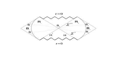
Figure 1: This is a Penrose diagram for the Schwarzschild wormhole.

We denote with $\Sigma_{t}$ the $t=constant$ hypersurface. Any of such hypersurfaces is invariant under $T$-reflections and has Einstein-Rosen bridge topology $R^{1}\times S^{2}$, represented in Fig.$\left(\ref{wormhole}\right)$, whose intrinsic geometry and time derivatives are chosen to satisfy the gravitational constraint equations

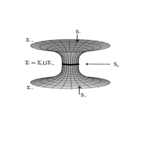
Figure 2: Wormhole representation for the Schwarzschild metric. The bifurcation surface $S_{0}$ divides the hypersurfaces $\Sigma_{+}$ and $\Sigma_{-}$.

We denote by ${\Sigma}_{\pm}$ the parts of ${\Sigma}$ lying in $R_{\pm}$ respectively. The line element $\left(\ref{Kruskal}\right)$ restricted to the surface ${\Sigma}$ reads

$$dl^{2}=dy^{2}+r^{2}(y)d\Omega^{2}\ ,$$ (8)

where the quantity $y$, defined by

$$dy=\pm\frac{dr}{\sqrt{1-2MG/r}},$$ (9)

represents the proper geodesic distance from the “throat” of the bridge located at $r=r(y=0)=r_{+}=2MG$. We choose $y$ to be positive in ${\Sigma}_{+}$ and negative in ${\Sigma}_{-}$. The set $(t,y,\theta,\phi)$ can be used as canonical coordinates everywhere in $R_{\pm}$ outside the bifurcation surface ${S}_{0}$. These coordinates are right-oriented in $R_{+}$ and left-oriented in $R_{-}$. The configuration we wish to examine is described by boundary surfaces located in different regions with two different slices ${\Sigma}^{\prime}$ $\equiv\Sigma_{t^{\prime}}$ and ${\Sigma}^{\prime\prime}\equiv\Sigma_{t^{\prime\prime}}$ intersecting at the same two-dimensional bifurcation sphere ${S}_{0}$. We call this sequence of slices ${\Sigma}_{t}$ (defined by the equation $t=\mathrm{constant}$, with $t^{\prime}\leq t\leq t^{\prime\prime}$) a “tilted foliation”FroMar . For a “tilted foliation” the spacetime domain $M$ lying between ${\Sigma}^{\prime}$ and ${\Sigma}^{\prime\prime}$ consists of two wedges $\mathcal{M}_{+}$ and $\mathcal{M}_{-}$ located in the right ($R_{+}$) and left ($R_{-}$) sectors of the Kruskal diagram. The region $\mathcal{M}=\mathcal{M}_{+}\cup\mathcal{M}_{-}$ is bounded by $\Sigma^{\prime}$ and $\Sigma^{\prime\prime}$ and by a three-dimensional timelike boundary $B$ that consists of two disconnected parts $B_{+}$ and $B_{-}$. For a general eternal black hole geometry the boundaries $B_{+}$ and $B_{-}$ are located in $\mathcal{M}_{+}$ and $\mathcal{M}_{-}$, respectively. We define ${S_{\pm}^{2}=}\Sigma_{\pm}\cap{B_{\pm}}$. The topology of the slices $\Sigma$ is therefore $I_{\Sigma}\times S^{2}$, where $I_{\Sigma}$ is a finite spacelike distance, while the topology of ${B_{\pm}}$ is $I_{t}\times S_{\pm}^{2}$, where $I_{t}$ is a finite timelike distance. In Schwarzschild coordinates the line element of Eq.$\left(\ref{Kruskal}\right)$ can be written as

$$ds^{2}=-N^{2}dt^{2}+dy^{2}+r^{2}\left(y\right)d\Omega^{2},$$ (10)

where $y$ is the proper radial distance from the throat defined in Eq.$\left(\ref{propdist}\right)$. The coordinate $y$ covers the entire range $\left(-\infty,+\infty\right)$. $N$ is the corresponding lapse function written in terms of the proper distance from the throat

$$N^{2}=1-\frac{2MG}{r\left(y\right)}.$$ (11)

We define the four-velocity vector with $u_{\mu}=-N\partial_{\mu}t$, while the timelike unit vector normal to the hypersurface $\Sigma_{t\,}$ is $u^{\mu}$. This is chosen to be future oriented in $\mathcal{M}$ and normalized by the condition $u\cdot u=-1$. The lapse $N$ is positive at $\Sigma_{+}$, negative at $\Sigma_{-}$ and vanishing at the bifurcation surface. The spacelike normal $n^{\mu}$ to the three-dimensional boundaries $B{{}_{\pm}}$, is defined to be outward pointing at $B{{}_{+}}$, inward pointing at $B{{}_{-}}$, and normalized so that $n\cdot n=1$ with the further condition $\left.\left(u\cdot n\right)\right|_{{B_{\pm}}}=0$. Following Ref.FroMar , greek indices are used for tensors in $\mathcal{M}$ while latin indices are used for tensors defined in either $\Sigma$ or $B{{}_{\pm}}$. The metric and extrinsic curvature of $\Sigma$ as a surface embedded in $\mathcal{M}$ are denoted by $h_{ij}$ and $K_{ij}=-h_{i}^{k}\nabla_{k}u_{j}$, respectively, while the metric and extrinsic curvature of the boundaries ${B_{\pm}}$ as surfaces embedded in $\mathcal{M}$ are $\gamma_{ij}$ and $\Theta_{ij}=-\gamma_{i}^{k}\nabla_{k}n_{j}$. Covariant differentiation with respect to the metric $g_{\mu\nu}$ and $h_{ij}$ is denoted by $\nabla$ and $D$, respectively. The induced metric and extrinsic curvature of the boundaries ${S_{\pm}^{2}}$ as surfaces embedded on $\Sigma$ are denoted by $\sigma_{ab}$ and $k_{ab}=-\sigma_{a}^{k}D_{k}n_{b}$, respectively, $\left(a,b=2,3\right)$. Explicitly, the metric tensors for the different surfaces are

$$h_{\mu\nu}=g_{\mu\nu}+u_{\mu}u_{\nu},\qquad\gamma_{\mu\nu}=g_{\mu\nu}-n_{\mu}n_{\nu},\qquad\sigma_{\mu\nu}=g_{\mu\nu}+u_{\mu}u_{\nu}-n_{\mu}n_{\nu}.$$ (12)

The determinants of the metric tensors are related by

$$\begin{array}[c]{c}\sqrt{-g}=\left|N\right|\sqrt{h},\\ \sqrt{-\gamma}=\left|N\right|\sqrt{\sigma}.\end{array}$$ (13)

The covariant form for the gravitational action generated by a tilted foliation with fixed three-dimensional boundary of $\mathcal{M}$ is

$$S=\frac{1}{2\kappa}\int_{\mathcal{M}_{+}}d^{4}x\,\sqrt{-g}\,\Re-\frac{1}{\kappa}\int_{B_{+}}d^{3}x\,\sqrt{-\gamma}\left(\,\Theta-\,\Theta_{0}\right)_{+}$$

$$-\frac{1}{2\kappa}\int_{\mathcal{M}_{-}}d^{4}x\,\sqrt{-g}\,\Re-\frac{1}{\kappa}\int_{B_{-}}d^{3}x\,\sqrt{-\gamma}\left(\,\Theta-\,\Theta_{0}\right)_{-},$$ (15)

where $\Re$ denotes the four-dimensional scalar curvature, $\kappa\equiv 8\pi G$. The integrations are taken over the coordinates $x^{\mu}$ which have the same orientation as the canonical coordinates $(t,y,\theta,\phi)$ of the tilted foliation. The differing signs in $\mathcal{M}_{+}$ and $\mathcal{M}_{-}$ reflect the fact that the coordinates have different time orientations in $\mathcal{M}_{+}$ and $\mathcal{M}_{-}$. The subtraction term

$$S_{0\left(\pm\right)}={\frac{1}{\kappa}}\int_{{B_{\pm}}}d^{3}x\,\sqrt{-\gamma}\,\Theta_{0}$$ (16)

is the extrinsic curvature evaluated on the reference space, which in this case has been chosen to be flat. The effect of $S_{0\left(\pm\right)}$ is to normalize the energy $E$ to zero for the Schwarzschild wormhole with $M=0$. In the next section we will carefully examine the contribution of the volume terms of the action. Here, we restrict the evaluation on the boundaries $B_{\pm}$ obtaining

$$S=-\frac{1}{\kappa}\int_{B_{+}}d^{3}x\,\sqrt{-\gamma}\left(\,\Theta-\,\Theta_{0}\right)_{+}-\frac{1}{\kappa}\int_{B_{-}}d^{3}x\,\sqrt{-\gamma}\left(\,\Theta-\,\Theta_{0}\right)_{-}.$$ (17)

The trace of the extrinsic curvature is

$$\Theta_{|_{\pm}}=-\nabla_{k}n^{k}=-\frac{1}{\sqrt{-g}}\partial_{k}\left(\sqrt{-g}g^{kj}n_{j}\right)=-\frac{1}{\left|N\right|r^{2}}\partial_{y}\left(\left|N\right|r^{2}\right).$$ (18)

With the help of Eqs.$\left(\ref{propdist}\right)$ and $\left(\ref{lapse}\right)$, we can write

$$\frac{\partial\left|N\right|}{\partial y}=\pm\frac{MG}{r^{2}\left(y\right)}\qquad\text{in }\Sigma_{\pm},$$ (19)

where we have used

$$\frac{\partial r}{\partial y}=\pm\sqrt{1-\frac{2MG}{r\left(y\right)}}\qquad\text{in }\Sigma_{\pm}.$$ (20)

Thus Eq.$\left(\ref{trace}\right)$ becomes

$$\Theta_{|_{\pm}}=\mp\frac{1}{\left|N\right|r^{2}\left(y\right)}\left[2r\left(y\right)-3MG\right],$$ (21)

while the subtraction term can be defined by

$$\Theta_{0|_{\pm}}=\lim_{M\rightarrow 0}\Theta_{|_{\pm}}=\mp\frac{2}{r}$$ (22)

and

$$\left(\Theta-\,\Theta_{0}\right)_{\pm}=\mp\frac{1}{\left|N\right|r^{2}\left(y\right)}\left[2r\left(y\right)-3MG-2\frac{r^{2}\left(y\right)}{r}\left|N\right|\right].$$ (23)

The proper “time” length in Eq.$\left(\ref{a4}\right)$ is

$${\frac{1}{\kappa}}\int_{{B}_{\pm}}dt\left|N\right|={\frac{1}{\kappa}T}\left|N\left(y_{\pm}\right)\right|\qquad\text{in }\Sigma_{\pm},$$ (24)

where $y_{\pm}$ is the location of the spatial boundary on $B_{\pm}$ and $T=t^{\prime\prime}-t^{\prime}$. The substitutions $t\rightarrow-i\tau$ and $N\rightarrow-iN_{E}$ do not modify the behavior of the boundary action in the Euclidean context. Thus Eq.$\left(\ref{a4a}\right)$ becomes

$$\beta_{\pm}=T_{\pm}^{-1}=N_{E}\left(r_{\pm}\right)\beta^{\ast}\qquad\text{in }\Sigma_{\pm},$$ (25)

where $r_{\pm}$ stands for $r\left(y_{\pm}\right)$ and where we have integrated over the period $\beta^{\ast}=8\pi MG$ obtained by imposing regularity condition on the horizon. Note that the inverse temperature at infinity is the same in both wedges. The difference between $\beta_{+}$ and $\beta_{-}$ essentially arises from the Tolman law involving the different location of the boundaries. Then the total action contribution is

$$S_{{B}_{\pm}}=\pm{\frac{4\pi}{\kappa}T}\left[2r-3MG-2rN_{E\pm}\right]|_{r=r_{\pm}}\longrightarrow I_{{B}_{\pm}}=\mp\left(8\pi Mr-12\pi M^{2}G-\beta r/G\right)|_{r=r_{\pm}}.$$ (26)

Like in the case of the Hamiltonian discussed in Ref.FroMar , the tree level action for the Schwarzschild wormhole can be cast in the form

$$\frac{1}{\kappa}\left(I_{+}-I_{-}\right)=\left(12\pi M^{2}G-8\pi Mr_{+}+\beta_{+}r_{+}/G\right)-\left(12\pi M^{2}G-8\pi Mr_{-}+\beta_{-}r_{-}/G\right).$$ (27)

From Eq.$\left(\ref{a5}\right)$, we can compute the energy of the system at the fixed temperature $\beta_{\pm}$ in each wedge. This is obtained by regarding Eq.$\left(\ref{a5}\right)$ as a function of $r$ and $T$ rather than of $r$ and $M$. We obtain

$$\begin{array}[c]{cc}E_{+}=\frac{\partial I_{+}}{\partial\beta_{+}}&=\frac{1}{G}\left[r_{+}-r_{+}\sqrt{1-2MG/r_{+}}\right]\\ E_{-}=\frac{\partial I_{-}}{\partial\beta_{-}}&=\frac{1}{G}\left[r_{-}-r_{-}\sqrt{1-2MG/r_{-}}\right]\end{array}.$$ (28)

Note that each term tends asymptotically to the Arnowitt-Deser-Misner $(\mathcal{ADM})$ massADM . Note also that if the boundary location is different in the respective wedge, implies that $E_{+}\neq E_{-}$. Nevertheless for the entropy we discover

$$\begin{array}[c]{cc}S_{+}=\beta_{+}\frac{\partial I_{+}}{\partial\beta_{+}}-I_{+}&=\beta_{+}E_{+}-I_{+}=4\pi M^{2}G\\ S_{-}=\beta_{-}\frac{\partial I_{-}}{\partial\beta_{-}}-I_{-}&=\beta_{-}E_{-}-I_{-}=4\pi M^{2}G\end{array},$$ (29)

namely it is independent on the wedge. This is a consequence of the definition we have used for computing the entropy. The same result has been obtained by Martinez in Ref.Martinez in the context of microcanonical approach to the entropy of an eternal black hole. Note that if one adopts the method used in Ref.Martinez for computing the entropy, it is not immediate to arrive at the result of Eq.$\left(\ref{a7}\right)$. By means of Eq.$\left(\ref{a7}\right)$, Eq.$\left(\ref{a5}\right)$ can be explicitly rewritten as

$$\beta_{+}E_{+}-\beta_{-}E_{-}=8\pi MG\left(N_{E+}E_{+}-N_{E-}E_{-}\right)=\beta^{\ast}\left(M_{+}-M_{-}\right).$$ (30)

Note that $\beta^{\ast}$ is the periodically identified “asymptotic Euclidean time” which is independent on the considered wedge. We can recognize three different cases

1. $M_{+}>M_{-}$. The limit case is when $r_{+}\rightarrow\infty\left(y_{+}\rightarrow+\infty\right)$, while $r_{-}=2GM\left(y_{-}=0\right)$. This corresponds to $M_{+}=M_{\mathcal{ADM}}$ and $M_{-}=0$. This situation is the standard one, where the black hole thermodynamics is investigated in the wedge $\mathcal{M}_{+}$. Indeed

2. $M_{+}<M_{-}$. The limit case is when $r_{-}\rightarrow\infty\left(y_{-}\rightarrow-\infty\right)$, while $r_{+}=2GM\left(y_{+}=0\right)$. This corresponds to $M_{-}=M_{\mathcal{ADM}}$ and $M_{+}=0$. This situation is “dual” to the previous in the sense that the black hole thermodynamics is investigated in the wedge $\mathcal{M}_{-}$.

3. $M_{+}=M_{-}$.The left boundary $y_{-}$ and the right boundary $y_{+}$ are symmetric with respect to the bifurcation surface $S_{0}^{2}$, which implies that $r_{+}=r_{-}$.

Case 3 corresponds to a vanishing action. Nevertheless, it is well known that a vanishing action with a Euclidean metric describes flat spaceSchoenYau1 . Therefore, in this very particular case we have found an alternative way to flat space at the price of having a topology change.

III Nonconformal Negative Modes

The measure of stability in this approach is the eigenvalue spectrum of the nonconformal perturbative modes for the solution. Should there be a mode with a negative eigenvalue, then the action for this solution is a saddle-point in its phase space rather than a true minimum. Consequently, there ought to be a correspondence between the presence of such a negative mode and the local thermodynamic stability as governed by the heat capacity. Negative modes arise from the analysis of geometric fluctuations about classical Euclidean solutions of the Einstein field equations. However, the analysis to confirm their existence must be performed with care, since the gauge freedom of the Euclidean action will in general introduce a large number of non-physical negative modes associated with conformal deformations of the metric. For pure gravity, the contributions from the conformal and the nonconformal modes decouple if a suitable gauge is chosen. In the path integral approach Hawking , the partition function $Z$ is generally defined as a functional integral over all metrics with some fixed asymptotic behavior on some manifold $\mathcal{M}$,

$$Z=\int_{\mathcal{M}}D[g]\exp\left(-iS[g]\right).$$ (31)

This integral is formally defined by an analytic continuation to a Euclidean section of $\mathcal{M}$ denoted by $\mathcal{\bar{M}}$, where the right and left wedges of a Lorentzian eternal black hole (wormhole) are mapped into two complex sectors $\mathcal{\bar{M}}_{+}$ and $\mathcal{\bar{M}}_{-}$ to become

$$Z=\int_{\mathcal{\bar{M}}}D[g]\exp\left(-I\left[g\right]\right),$$ (32)

where the integral is performed over all positive definite metrics $g$. In the case of pure gravity, the Euclidean action comes from Eq.$\left(\ref{a3}\right)$ whose expression is

$$I=-{\frac{1}{2\kappa}}\int_{\mathcal{\bar{M}}_{+}}d^{4}x\,\sqrt{g}\,R+{\frac{1}{\kappa}}\int_{\partial\mathcal{\bar{M}}{{}_{+}}}d^{3}x\,\sqrt{\gamma}\left(\,\Theta-\,\Theta_{0}\right)$$

$$+{\frac{1}{2\kappa}}\int_{\mathcal{\bar{M}}_{-}}d^{4}x\,\sqrt{g}\,R+{\frac{1}{\kappa}}\int_{\partial\mathcal{\bar{M}}_{-}}d^{3}x\,\sqrt{\gamma}\left(\,\Theta-\,\Theta_{0}\right).$$ (33)

This partition function may be approximated using saddle-point techniques, by Taylor expanding about the known stationary points of the Euclidean action – the solutions to the Einstein field equations

$$R_{\mu\nu}=0.$$ (34)

The expansions are performed by writing the metric $g_{ab}$ as

$$g_{\mu\nu}=\bar{g}_{\mu\nu}+h_{\mu\nu}$$ (35)

with $h_{\mu\nu}$ treated as a quantum field on the classical fixed background $\bar{g}_{\mu\nu}$ which vanishes on the boundary $\partial\mathcal{\bar{M}}_{\pm}$. Thus the Euclidean action becomes

$$I[g]=I[\bar{g}]_{+}+I_{2}[h]_{+}-I[\bar{g}]_{-}-I_{2}[h]_{-}+\cdots$$ (36)

where the linear term $I_{1}$ vanishes precisely because $\bar{g}_{\mu\nu}$ is a classical solution, $I_{2}$ is quadratic in the field $h_{\mu\nu}$ in each complex sector, and ‘$\cdots$’ represents terms of higher than quadratic order. The Taylor expansion of the action in $\mathcal{\bar{M}}=\mathcal{\bar{M}}_{+}\cup\mathcal{\bar{M}}_{-}$ leads to the following one loop approximation of the partition function

$$\log Z=-I\left[\bar{g}\right]_{+}+\log\int_{\mathcal{\bar{M}}_{+}}D\left[h\right]_{+}\exp\left(-I_{2}\left[h\right]_{+}\right)+I\left[\bar{g}\right]_{-}+\log\int_{\mathcal{\bar{M}}_{-}}D\left[h\right]_{-}\exp\left(I_{2}\left[h\right]_{-}\right).$$ (37)

It is interesting to note that in this form the gravitational quantum fluctuations on $\mathcal{\bar{M}}_{+}$ $\left(\mathcal{\bar{M}}_{-}\right)$ act as a sort of source field with respect to $\mathcal{\bar{M}}_{-}\left(\mathcal{\bar{M}}_{+}\right)$. The quadratic contribution to the action is straightforward to evaluate, and may be written for arbitrary $h_{\mu\nu}$ in each wedge, in the form

$$I_{2}[h]_{\pm}=\frac{1}{4\kappa}\int d^{4}x\sqrt{g}h_{\pm}^{\mu\nu}G_{\mu\nu\rho\sigma}h_{\pm}^{\rho\sigma}.$$ (38)

$G$ is a physical gauge invariant spin-2 operator which acts on the transverse and trace-free part of $h_{\mu\nu}$ and takes the simple form

$$G_{\mu\nu\rho\sigma}=-g_{\mu\rho}g_{\nu\sigma}\nabla_{\alpha}\nabla^{\alpha}-2R_{\mu\rho\nu\sigma}.$$ (39)

In general, $G$ will have some finite number – generally zero or one – of negative eigenvalues, which correspond to the nonconformal negative modes of the solution. The eigenvalues of $G$ are determined by all solutions to the elliptic equation

$$G_{\rho\sigma}^{\mu\nu}h_{(n)}^{\rho\sigma}=\lambda_{(n)}h_{(n)}^{\mu\nu}$$ (40)

where the eigenfunctions $h_{\mu\nu}$ are real, regular, symmetric, transverse, trace-free, and normalizable tensors. Clearly, should one of the eigenvalues of $G$ be negative, then the product of all of the eigenvalues would also be negative. The contribution to $\log Z$ from fluctuations about the classical solution would then contain an imaginary component, leading to an instability in the ensemble similar to the type proposed by Gross, Perry and Yaffe GPY . Naively, then, the one-loop term may be written as $\frac{1}{2}\log Det(\mu^{-2}G)$ where $\mu$ is a regularization mass, and the determinant is formally defined as the product of the eigenvalues of $G$. However, due to the diffeomorphism gauge freedom of the action, $A$ will in general have a large number of zero eigenvalues, and so this procedure as stated is ill-defined. The remedy is to add a gauge fixing term $B$ – such that the operator $A+B$ has no zero eigenvalues – and an associated ghost contribution $C$, to obtain

$$\log Z=-I[g]-\frac{1}{2}\log Det(\mu^{-2}\{A+B\})+\log Det(\mu^{-2}C).$$ (41)

Such terms may be dealt with by means of generalized zeta functions, as considered by Gibbons, Hawking, and Perry GHP , and extended to include a $\Lambda$ term by Hawking Hawking . In order that this be possible, the terms must be expressed as sums of operators, each with only a finite number of negative eigenvalues. This may be achieved by writing $A+B$ as $-F+G$, where $F$ is a scalar operator acting on the trace of $h_{\mu\nu}$. The ghost term $C$ is a spin-1 operator acting on divergence-free vectors, and An observation of primary significance is that a gauge may be chosen in which the operators $F$ and $C$ have no negative eigenvalues. If the background metric $g_{ab}$ is flat then, in addition, $G$ will be positive-definite, but for a non-flat background this is not the case.

IV Variational Approach to the Negative Mode

Following the treatment given in GPY , and subsequently in Allen for the Schwarzschild case, it is clear that only spherically symmetric and $\tau$-independent solutions of Eq.$\left(\ref{eigenvalue}\right)$ need be considered as candidate nonconformal negative modes. In static and spherically symmetric backgrounds, modes of higher multipole moment will necessarily have greater eigenvalues. With this assumption, it is then straightforward to write down a construction for such solutions to $G$ valid in a four-dimensional Euclidean wormhole background of the form $\left(\ref{a1a}\right)$. Since $G$ acts only on symmetric transverse and trace-free tensors, then clearly the constructed solutions must exhibit all of these properties. If the mode $h_{\mu\nu}^{\pm}$ is written in the manifestly trace-free and symmetric form

$$\left(h_{\nu}^{\mu}\right)^{\pm}=diag\left(H_{0}^{\pm}(y),H_{1}^{\pm}(y),-\frac{1}{2}\left(H_{0}^{\pm}(y)+H_{1}^{\pm}(y)\right),-\frac{1}{2}\left(H_{0}^{\pm}(y)+H_{1}^{\pm}(y)\right)\right),$$ (42)

then the final property, $\nabla^{a}h_{\mu\nu}^{\pm}=0$, is guaranteed if it is further assumed that $H_{0}^{\pm}(y)$ and $H_{1}^{\pm}(y)$ are related through the first order equation

$$H_{1,y}^{\pm}+\frac{3}{r}r_{,y}H_{1}^{\pm}+\frac{N_{,y}}{N}H_{1}^{\pm}=\frac{N_{,y}}{N}H_{0}^{\pm}-\frac{3}{r}r_{,y}H_{0}^{\pm}.$$ (43)

In Eqs.$\left(\ref{tracefree}\right)$ and $\left(\ref{transverse}\right)$, we have explicitly written the location of the perturbation on each patch covering one universe. The two patches join at the throat of the wormhole and the transversality condition can be cast into the form

$$\left[\frac{dH_{1}^{\pm}(r)}{dr}+\frac{3}{r}H_{1}^{\pm}(r)+\frac{1}{N}\frac{dN}{dr}H_{1}^{\pm}(r)\right]\frac{dr}{dy}=\left[\frac{1}{N}\frac{dN}{dr}H_{0}^{\pm}(r)-\frac{3}{r}H_{0}^{\pm}(r)\right]\frac{dr}{dy},$$ (44)

where it is manifest the independence on the wedge location. This is a consequence of the discrete symmetry $\left(\ref{discrete}\right)$ between the asymptotically flat wedges. When we apply this symmetry to the the eigenvalue equation $\left(\ref{diff_eq}\right)$ with the help of the following substitution

$$N \rightarrow-N$$

$$r_{,y} \rightarrow-r_{,y},$$

we find that Eq.$\left(\ref{diff_eq}\right)$ is invariant in form only on the coordinate $r$. With the ansatz $\left(\ref{tracefree}\right)$ and $\left(\ref{transverse1}\right)$, the eigenvalue equation $\left(\ref{eigenvalue}\right)$ reduces to a linear second order ordinary differential equation for the component $H_{1}^{\pm}\left(y\right)$ and eigenvalue $\mu^{2}.$ To further proceed, we insert Eqs.$\left(\ref{propdist}\right)$ and $\left(\ref{lapse}\right)$ into Eq.$\left(\ref{eigenvalue}\right)$. Since we have chosen $y$ and the Euclidean lapse $N_{E}$ to be positive in $\mathcal{\bar{M}}_{+}$ and negative in $\mathcal{\bar{M}}_{-}$, then Eq.$\left(\ref{eigenvalue}\right)$ is separated in two pieces

$$\frac{d^{2}H_{1}\left(y\right)}{dy^{2}}+b^{\pm}\left(y\right)\frac{dH_{1}\left(y\right)}{dy}+a^{\pm}\left(y\right)H_{1}\left(y\right)=-\mu^{2}H_{1}\left(y\right),$$ (45)

where

$$b^{+}\left(y\right)=\sqrt{1-\frac{2\,MG}{r\left(y\right)}}\frac{\left(4\,r^{2}\left(y\right)-23\,MGr\left(y\right)+27\,M^{2}G^{2}\right)}{r^{2}\left(y\right)\left(r\left(y\right)-2\,MG\right)\left(r\left(y\right)-3\,MG\right)}\qquad a^{+}\left(y\right)=\frac{8MG}{\left(r\left(y\right)-3\,MG\right)r^{2}\left(y\right)}$$ (46)

in $\mathcal{\bar{M}}_{+}$ and

$$b^{-}\left(y\right)=-\frac{\left(4\,r^{2}\left(y\right)-23\,MGr\left(y\right)+27\,M^{2}G^{2}\right)}{r^{2}\left(y\right)\left(r\left(y\right)-3\,MG\right)\sqrt{1-2\,MG/r\left(y\right)}}\qquad a^{-}\left(y\right)=\frac{8MG}{\left(r\left(y\right)-3\,MG\right)r^{2}\left(y\right)}$$ (47)

in $\mathcal{\bar{M}}_{-}$. After having cast Eq.$\left(\ref{diff_eq}\right)$ in the standard Sturm-Liouville form, we apply a variational procedure to establish the existence of an instability by means of trial functions. The standard Sturm-Liouville form of Eq.$\left(\ref{diff_eq}\right)$ is

$$\frac{d}{dy}\left(p^{\pm}\left(y\right)\frac{d}{dy}H_{1}\left(y\right)\right)+q^{\pm}\left(y\right)H_{1}\left(y\right)+\mu^{2}p^{\pm}\left(y\right)H_{1}\left(y\right)=0,$$ (48)

where the integrating factor $p^{\pm}\left(y\right)$ is defined by

$$p^{\pm}\left(y\right)=\exp\int b^{\pm}\left(y\right)dy=\exp\pm\int\frac{b^{\pm}\left(r\left(y\right)\right)}{\sqrt{1-2\,MG/r\left(y\right)}}dr=\frac{\left(r\left(y\right)\right)^{9/2}\left(r\left(y\right)-2\,MG\right)^{3/2}}{\left(r\left(y\right)-3\,MG\right)^{2}}.$$ (49)

To compute the integrating factor we used Eq.$\left(\ref{propdist}\right)$. The coefficient

$$q^{\pm}\left(y\right)=p^{\pm}\left(y\right)a^{\pm}\left(y\right)$$ (50)

and the boundary conditions

$$\left.p^{+}\left(y\right)\frac{dH_{1}\left(y\right)}{dy}H_{1}\left(y\right)\right|_{y=0}^{y=+\infty}\qquad\text{and\qquad}\left.p^{-}\left(y\right)\frac{dH_{1}\left(y\right)}{dy}H_{1}\left(y\right)\right|_{y=-\infty}^{y=0},$$ (51)

lead us to write the Sturm-Liouville problem in the following functional form

$$F\left[H_{1}\left(y\right);\lambda\right]=\frac{N\left[H_{1}\left(y\right);\lambda\right]}{D\left[H_{1}\left(y\right);\lambda\right]}=\mu_{\pm}^{2}\left(\lambda\right)=\frac{-\int_{I_{\pm}}dyp^{\pm}\left(y\right)\left(\frac{d}{dy}H_{1}\left(y\right)\right)^{2}+\int_{I_{\pm}}dyq^{\pm}\left(y\right)H_{1}^{2}\left(y\right)}{\int_{I_{\pm}}dyp^{\pm}\left(y\right)H_{1}^{2}\left(y\right)},$$ (52)

where $I_{+}\equiv\left[0,+\infty\right)$ and $I_{-}\equiv\left(-\infty,0\right]$. The choice of a trial function is suggested by the asymptotic behavior of in Eq.$\left(\ref{diff_eq}\right)$. Indeed, when $y\rightarrow\pm\infty,$ $H_{1}^{\pm}\left(y\right)\simeq\exp\left(\mp\lambda y\right)\simeq\exp\left(-\lambda r\right)$. The denominator in Eq.$\left(\ref{Var}\right)$ compensates the lack of normalization in the trial function $H_{1}^{\pm}\left(y\right)$. If $\lambda$ is defined as a variational parameter, then the Rayleigh-Ritz method leads to the following result

$$\mu_{\pm}^{2}\left(\lambda_{\min}\right)=-.1374637652\qquad for\qquad\lambda_{\min}=.4471243737.$$ (53)

However the denominator of Eq.$\left(\ref{Var}\right)$ vanishes for $\bar{\lambda}=1.360771766$ and for $\lambda>\bar{\lambda}$, the “normalization” changes sign. The lack of positivity for every $\lambda$ is related to the appearance of a spurious singularity in $r=3MG$. Therefore, it is necessary to choose a better form for the trial function $H_{1}^{\pm}\left(y\right)$ which partially removes the singularity in $r=3MG$. Such a form is given by $H_{1}^{\pm}\left(y\right)\simeq H_{1}\left(r\right)=\exp\left(-\lambda r\right)\left(r-3\,MG\right)$. With this choice, the “normalization” is strictly positive for every $\lambda$. The minimum of $\mu_{\pm}^{2}\left(\lambda\right)$ is reached for $\lambda_{\min}=.9223711858$ and $\mu_{\pm}^{2}\left(\lambda_{\min}\right)=-.3827139389$. It is interesting to note that

$$\mu^{2}\left(\lambda_{\min}\right)=\mu_{+}^{2}\left(\lambda_{\min}\right)+\mu_{-}^{2}\left(\lambda_{\min}\right)=-0.765\,44\rightarrow\mu^{2}\left(\lambda_{\min}\right)/\left(2MG\right)^{2}=-0.191\,36/\left(MG\right)^{2}.$$ (54)

This is the same value obtained by GPY for a single Euclidean black hole.

V Summary and Conclusions

In this paper we have analyzed, the one loop contribution coming from quantum fluctuations around a background metric describing a Schwarzschild wormhole which has boundary terms in both wedges of the Penrose diagram. Usually, this kind of analysis is performed only in the $R_{+}$ wedge of diagram $\left(\ref{penrose}\right)$. However, due to the symmetry property of transformation $\left(\ref{discrete}\right)$, a contribution from region $R_{-}$ is not unexpected. Moreover, the possibility of a fine tuning between boundaries in the opposite regions gives the opportunity to vanish the classical gravitational action. The vanishing of the classical action leads to the interpretation that we are dealing with flat space. On the other hand the presence in each wedge of a term proportional to the ADM mass is a signal that a non flat configuration has been taken under examination. An interpretation of this puzzling situation can be given in terms of black hole pair creation mediated by a wormhole, with the pair elements residing in the different universes. This proposal is not completely new and it has been investigated in Refs.Remo in a Hamiltonian formulation, where a foliation of the manifold $\mathcal{M}$ is crucial. On the other hand, the action formalism has the advantage of being fully covariant. However, the vanishing of the classical action is not sufficient to establish if spacetime will produce a pair or will persist in its flat configuration. It is, therefore necessary to discover if the one loop approximation will produce an instability. The variational approach we have used for the Sturm-Liouville problem in the TT sector has shown an unstable mode in the s-wave approximation in both wedges. This is the signal that flat space is not only unstable when the space is furnished with a temperature $T=1/\left(8\pi MG\right)$, but is even unstable with respect to Schwinger pair creation. One possible conclusion is that flat space can be no more considered as the general accepted vacuum of quantum gravity and the instability with respect to Schwinger pair suggests to search in this direction instead of rejecting the result with the further motivation that this instability can disappear if the bounding box is restricted enough. A partial success in this direction has been obtained by AllenAllen in terms of hot quantum gravity from one side. On the other side, the choice of a non-trivial vacuum formed by a large number of black hole pair generated in the same way we have investigated in this paper has led to a possible stable picture of space time foam, which could replace flat space as a candidate for the quantum gravity vacuumRemo1 .

VI Acknowledgments

I wish to thank M. Cadoni, R. Casadio, M. Cavaglià, V. Moretti and S. Mignemi for useful comments and discussions.

Appendix A Searching for Eigenvalues with the Rayleigh-Ritz method

In this Appendix, we will explicitly solve the eigenvalue problem of Eq.$\left(\ref{Var}\right)$ with the Rayleigh-Ritz method. We here report two principal choices of trial wave functions:

1. $H_{1}^{\pm}\left(y\right)=\exp\left(\mp\lambda y\right)\rightarrow\exp\left(-\lambda r\right)$. For this choice Eq.$\left(\ref{Var}\right)$ becomes,

   $$\mu^{2}\left(\lambda\right)=\lambda^{2}-8MG\frac{\int_{2MG}^{+\infty}dre^{-2\lambda r}\frac{r^{3}\left(r-2MG\right)}{\left(r-3MG\right)^{3}}}{\int_{2MG}^{+\infty}dre^{-2\lambda r}\frac{r^{5}\left(r-2MG\right)}{\left(r-3MG\right)^{2}}}=\lambda^{2}-\frac{A\left(\lambda\right)}{B\left(\lambda\right)},$$ (55)

   where

   $$A\left(\lambda\right)=8MG\int_{2MG}^{+\infty}dre^{-2\lambda r}\frac{r^{3}\left(r-2MG\right)}{\left(r-3MG\right)^{3}}=256\left(MG\right)^{3}\int_{1}^{+\infty}d\rho\exp\left(-2\tilde{\lambda}\rho\right)\frac{\rho^{3}\left(\rho-1\right)}{\left(2\rho-3\right)^{3}}$$

   $$=256\left(MG\right)^{3}\left[I_{3}^{4}\left(\tilde{\lambda}\right)-I_{3}^{3}\left(\tilde{\lambda}\right)\right]$$ (56)

   and

   $$B\left(\lambda\right)=\int_{2MG}^{+\infty}dre^{-2\lambda r}\frac{r^{5}\left(r-2MG\right)}{\left(r-3MG\right)^{2}}=128\left(MG\right)^{5}\int_{1}^{+\infty}d\rho\exp\left(-2\tilde{\lambda}\rho\right)\frac{\rho^{5}\left(\rho-1\right)}{\left(2\rho-3\right)^{2}}$$

   $$=128\left(MG\right)^{5}\left[I_{2}^{6}\left(\tilde{\lambda}\right)-I_{2}^{5}\left(\tilde{\lambda}\right)\right].$$ (57a)

   We have defined $$\rho=r/\left(2MG\right) \tilde{\lambda}=\lambda 2MG$$, and introduced the following function

   $$I_{m}^{n}\left(\tilde{\lambda}\right)=\int_{1}^{+\infty}d\rho\exp\left(-2\tilde{\lambda}\rho\right)\frac{\rho^{n}}{\left(2\rho-3\right)^{m}}=\left(-1\right)^{n}\frac{d^{n}I_{m}^{0}\left(\tilde{\lambda}\right)}{d\tilde{\lambda}^{n}}.$$ (58)

   $I_{m}^{0}\left(\tilde{\lambda}\right)$ can be easily integrated with the formulaGR

   $$\int_{u}^{+\infty}dx\frac{\exp\left(-\nu x\right)}{\left(x+\beta\right)^{m}}=\exp\left(-\nu u\right)\sum_{k=1}^{m-1}\frac{\left(k-1\right)!}{\left(m-1\right)!}\frac{\left(-\nu\right)^{m-k-1}}{\left(u+\beta\right)^{k}}-\frac{\left(-\nu\right)^{m-1}}{\left(m-1\right)!}\exp\left(\beta\nu\right)\operatorname{Ei}\left[-\left(u+\beta\right)\nu\right]$$ (59)

   with $m\geq 2$, $\left|\arg\left(u+\beta\right)\right|<\pi$ and $\operatorname{Re}\nu>0$. $\operatorname{Ei}\left(x\right)$ is the exponential function. We get $A\left(\lambda\right)=$

   $${\frac{\left(-18\,{\lambda}\,{e^{{\lambda}}}-108\,{\lambda}^{3}\operatorname{Ei}\left({\lambda}\right)+72\,{\lambda}^{2}\operatorname{Ei}\left({\lambda}\right)+81\,{\lambda}^{2}{e^{{\lambda}}}-27\,{\lambda}^{3}{e^{{\lambda}}}+27\,{\lambda}^{4}\operatorname{Ei}\left({\lambda}\right)-2\,{e^{{\lambda}}}\right){e^{-3\,{\lambda}}}}{8{\lambda}^{2}}}$$ (60)

   and $B\left(\lambda\right)=$

   $${\frac{\left(24\,{e^{{\lambda}}}-243\,{\lambda}^{5}{e^{{\lambda}}}+243\,{\lambda}^{6}\operatorname{Ei}\left({\lambda}\right)-648\,{\lambda}^{5}\operatorname{Ei}\left({\lambda}\right)+194\,{\lambda}^{3}{e^{{\lambda}}}+72\,{\lambda}\,{e^{{\lambda}}}+126\,{\lambda}^{2}{e^{{\lambda}}}+405\,{\lambda}^{4}{e^{{\lambda}}}\right){e^{-3\,{\lambda}}}}{128{\lambda}^{5}}.}$$ (61)

   $B\left(\lambda\right)$ vanishes for $\lambda=1.360771766$ and $\mu^{2}\left(\lambda\right)$ gets its minimum for $\lambda_{\min}=.4471243737$ leading to $\mu^{2}\left(\lambda_{\min}\right)=-.1374637652$

2. With the help of Eq.$\left(\ref{Formula}\right)$ and choosing $H_{1}^{\pm}\left(y\right)=\exp\left(\mp\lambda y\right)\left(r\left(y\right)-3MG\right)\rightarrow\exp\left(-\lambda r\right)\left(r-3MG\right)$ we get a more complicated form in $N\left[H_{1}\left(y\right);\lambda\right]$ of Eq.$\left(\ref{Var}\right)$, while $D\left[H_{1}\left(y\right);\lambda\right]$ is simpler. Indeed

   $$N\left[H_{1}\left(y\right);\lambda\right]=-\int_{2MG}^{+\infty}dr\frac{r^{5}\left(r-2\,MG\right)}{\left(r-3\,MG\right)^{2}}\left(\frac{d}{dr}\left[e^{-2\lambda r}\left(r-3MG\right)\right]\right)^{2}+8MG\int_{2MG}^{+\infty}dre^{-2\lambda r}\frac{r^{3}\left(r-2MG\right)}{\left(r-3MG\right)}$$

   $$=-\frac{\left(2MG\right)^{7}}{\left(2MG\right)^{2}}\int_{1}^{+\infty}d\rho\frac{\rho^{5}\left(\rho-1\right)}{\left(2\rho-3\right)^{2}}\left(\frac{d}{d\rho}\left[e^{-2\tilde{\lambda}\rho}\left(2\rho-3\right)\right]\right)^{2}+8MG\frac{\left(2MG\right)^{5}}{MG}\int_{1}^{+\infty}d\rho e^{-2\tilde{\lambda}\rho}\frac{\rho^{3}\left(\rho-1\right)}{\left(2\rho-3\right)}$$

   $$=-\,\left(2MG\right)^{5}{\frac{\left(243\,{\lambda}^{6}{Ei}\left({\lambda}\right)-239\,{\lambda}^{5}{e^{{\lambda}}}+42\,{e^{{\lambda}}}+225\,{\lambda}^{4}{e^{{\lambda}}}-432\,{\lambda}^{5}{Ei}\left({\lambda}\right)+86\,{\lambda}^{2}{e^{{\lambda}}}+102\,{\lambda}^{3}{e^{{\lambda}}}+78\,{\lambda}\,{e^{{\lambda}}}\right){e^{-3\,{\lambda}}}}{16{\lambda}^{5}}}$$ (62)

   and

   $$D\left[H_{1}\left(y\right);\lambda\right]=\int_{2MG}^{+\infty}dr\left[e^{-2\lambda r}r^{5}\left(r-2\,MG\right)\right]=\left(2MG\right)^{7}\int_{1}^{+\infty}d\rho\exp\left(-2\tilde{\lambda}\rho\right)\rho^{5}\left(\rho-1\right)$$

   $$=\left(2MG\right)^{7}{\frac{{e^{-2{\lambda}}}\left(45+2\,{\lambda}^{5}+10\,{\lambda}^{4}+30\,{\lambda}^{3}+60\,{\lambda}^{2}+75\,{\lambda}\right)}{8{\lambda}^{7}}.}$$ (63)

   Note the positiveness of $D\left[H_{1}\left(y\right);\lambda\right]$ for every $\lambda$, ensuring a correct normalization. The minimum of $\mu^{2}\left(\lambda\right)$ is reached in this case for $\lambda_{\min}=.9223711858$ and $\mu^{2}\left(\lambda_{\min}\right)=-.3827139389$.

References

• (1) R. Schoen, S.T. Yau, Commun. Math. Phys. 65, 45 (1979); Commun. Math. Phys. 79, 231 (1981).
• (2) R. Schoen and S.T. Yau, Phys. Rev. Lett. 42, 547 (1979).
• (3) E. Witten, Commun. Math. Phys. 80, 381 (1981).
• (4) D.J. Gross, M.J. Perry, & L.G. Yaffe, Phys. Rev. D 25 330 (1982).
• (5) S. Coleman, Nucl. Phys. B 298 (1988), 178; S. Coleman, Aspects of Symmetry (Cambridge University Press, Cambridge, 1985).
• (6) B. Allen, Phys. Rev. D 30 1153 (1984).
• (7) P. Ginsparg and M.J. Perry, Nucl. Phys. B 222 (1983) 245.
• (8) R.E. Young, Phys. Rev. D 28, (1983) 2436; R.E. Young, Phys. Rev. D 28 (1983) 2420.
• (9) M.S. Volkov and A. Wipf, Nucl. Phys. B 582 (2000), 313; hep-th/0003081.
• (10) S.W. Hawking and D.N. Page, Commun. Math. Phys. 87, 577 (1983).
• (11) T. Prestidge, Phys. Rev. D 61 (2000) 084002, hep-th/9907163.
• (12) E. Witten, Nucl Phys B195 481 (1982).
• (13) R. Gregory and R. Laflamme, Phys. Rev. D 37 305 (1988).
• (14) S.S. Gubser and I. Mitra, Instability of charged black holes in Anti-de Sitter space, hep-th/0009126; S.S. Gubser and I. Mitra, JHEP 8 (2001) 18. J.P. Gregory and S.F. Ross, Phys. Rev. D 64 (2001) 124006, hep-th/0106220. H.S. Reall, Phys. Rev. D 64 (2001) 044005, hep-th/0104071. G. Gibbons and S.A. Hartnoll, Phys. Rev. D 66 (2001) 064024, hep-th/0206202. I.P. Neupane, Phys. Rev. D 69 (2004) 084011, hep-th/0302132.
• (15) O.J.C. Dias and J.P. Lemos, Phys. Rev. D 69 (2004) 084006, hep-th/0310068; Phys. Rev. D 70 (2004) 024007, hep-th/0401069; Phys. Rev. D 70 (2004) 124023, hep-th/0410279.
• (16) R. Garattini, Nuovo Cimento B 113 (1998) 963, gr-qc/9609006. R. Garattini, Mod. Phys. Lett. A 13 (1998) 159, gr-qc/9801045. R. Garattini, Int. J. Mod. Phys. A 14 (1999) 2905, gr-qc/9805096. R. Garattini, Class. Quant. Grav. 18 (2001) 571, gr-qc/0012078.
• (17) R. Arnowitt, S. Deser, and C. W. Misner, in Gravitation: An Introduction to Current Research, edited by L. Witten (John Wiley & Sons, Inc., New York, 1962); B. S. DeWitt, Phys. Rev. 160, 1113 (1967).
• (18) R. Bousso and S.W. Hawking, Phys. Rev. D 52, 5659 (1995), gr-qc/9506047; R. Bousso and S.W. Hawking, Phys. Rev. D 54, 5659 (1995), gr-qc/9606052.
• (19) V.P. Frolov and E.A. Martinez, Class. Quant. Grav. 13 (1996) 481, gr-qc/9411001.
• (20) E.A. Martinez, Phys. Rev. D 51, 5732 (1995).
• (21) S.W Hawking, The Path-Integral Approach to Quantum Gravity, in General Relativity: An Einstein Centenary Survey, Ed. S.W Hawking & W. Israel (Cambridge University Press, Cambridge, 1979).
• (22) G.W Gibbons, S.W Hawking, & M.J. Perry, Nucl Phys B138 141 (1978).
• (23) T. Regge and J. A. Wheeler, Phys. Rev. 108, 1063 (1957).
• (24) C.V. Vishveshwara, Phys. Rev. D 1, 2870 (1970).
• (25) F. Zerilli, Phys. Rev. Lett. 24, 737 (1970).
• (26) W. Press and S.A. Teukolsky, Astrophys. J. 185, 649 (1973); 193, 443 (1974).
• (27) J.M. Stewart, Proc. R. Soc. London A 334, 51 (1975).
• (28) S. Chandrasekhar, The Mathematical Theory of Black Holes, (Oxford Science Publications, 1983).
• (29) R. Garattini, Nucl. Phys. Proc. Suppl. 88, 297 (2000), gr-qc/9910037. R. Garattini, Int. J. Mod. Phys. D 4, 635 (2002); Archive:gr-qc/0003090. R. Garattini, Int. J. Mod. Phys. A 17, 1965 (2002), Archive: gr-qc/0111068.
• (30) I.S. Gradshteyn and I.M. Ryzhik, Table of Integrals, Series, and Products (corrected and enlarged edition), edited by A. Jeffrey (Academic Press, Inc.).