The Power of General Relativity

Abstract

We study the cosmological and weak-field properties of theories of gravity derived by extending general relativity by means of a Lagrangian proportional to $R^{1+\delta}$. This scale-free extension reduces to general relativity when $\delta\rightarrow 0$. In order to constrain generalisations of general relativity of this power class we analyse the behaviour of the perfect-fluid Friedmann universes and isolate the physically relevant models of zero curvature. A stable matter-dominated period of evolution requires $\delta>0$ or $\delta<-1/4$. The stable attractors of the evolution are found. By considering the synthesis of light elements (helium-4, deuterium and lithium-7) we obtain the bound $-0.017<\delta<0.0012.$ We evaluate the effect on the power spectrum of clustering via the shift in the epoch of matter-radiation equality. The horizon size at matter–radiation equality will be shifted by $\sim 1\%$ for a value of $\delta\sim 0.0005.$ We study the stable extensions of the Schwarzschild solution in these theories and calculate the timelike and null geodesics. No significant bounds arise from null geodesic effects but the perihelion precession observations lead to the strong bound $\delta=2.7\pm 4.5\times 10^{-19}$ assuming that Mercury follows a timelike geodesic. The combination of these observational constraints leads to the overall bound $0\leq\delta<7.2\times 10^{-19}$ on theories of this type.

I Introduction

There is a long history of considering generalisations of Einstein’s theory of general relativity which reduce to general relativity in the weak gravity limit when the spacetime curvature, $R$, becomes small. Typically, these studies consider a gravitational Lagrangian which augments the linear Einstein-Hilbert Lagrangian by the addition of terms of quadratic or higher order in $R,$ first considered by Eddington edd ; these additions may also include terms in $\ln R$, gur . More general extensions of general relativity in this spirit have considered the structure of theories derived from gravitational Lagrangians that are general analytic functions of $R$, buch ; kerner ; BO ; magg . These choices produce theories which can look like general relativity plus small polynomial corrections in the appropriate limiting situations as $R$ becomes small. There has also been interest in theories with corrections to general relativity that are $O(R^{-1})$ because of their scope to introduce cosmological deviations from general relativity at late times which might mimic the effects of dark energy on the Hubble flow tur ; new . We also know that theories derived from a Lagrangian that is an analytic function of $R$ have an important conformal relationship to general relativity with scalar field sources so long as the trace of the energy-momentum tensor vanishes in the higher-order gravity theory CB ; maeda . All these theories introduce corrections to general relativity which come with a characteristic length scale that is determined by the new coupling constant that couples the higher-order terms to the Einstein-Hilbert part of the Lagrangian. In general, these theories are mathematically complicated with 4^th-order field equations that can exhibit singular perturbation behaviour unless care is taken to ensure that the stationary action does not become maximal rather than minimal ruz ; BO . and there are few interesting exact solutions other than those of general relativity, which are particular solutions in vacuum and for trace-free energy momentum tensor so long as the cosmological constant vanishes BO .

In this paper we are going to consider a different type of generalisation of Einstein’s general relativity, in which no new scale is introduced. The Lagrangian is proportional to $R^{n}$, and so general relativity is recovered in the $n\rightarrow 1$ limit, from above or below. Particular cases have been studied by Buchdahl Buc70 and Roxburgh rox . This gravitation theory has many appealing properties and, unlike other higher-order gravity theories, admits simple exact solutions for Friedmann cosmological models and exact static spherically symmetric solutions which generalise the Schwarzschild metric. As well as allowing comparison with observation these solutions also provide an interesting testing ground for new developments in gravitation theory such as particle production, holography and gravitational thermodynamics. Furthermore, this theory is of additional interest because it permits a very general investigation of the nature of its behaviour in the vicinity of a cosmological singularity which brings the behaviour of general relativity into sharper focus. In another paper Bar05 , we show that the counterpart of the Kasner anisotropic vacuum cosmology can be found exactly and strong conclusions drawn about the presence or absence of the chaotic behaviour found in the Mixmaster universe.

The structure of this paper is as follows; in the next section we present the gravitational action and field equations for the theory of gravity we will be considering. A conformal relationship with general relativity containing a scalar field in a Liouville (exponential) potential is then outlined and the Newtonian limit of the field equations is investigated. The rest of the paper is then split into two sections; the first investigates the cosmology of the theory and the second investigates the static and spherically symmetric weak field - in both cases our goal is to calculate predictions for physical processes, the results of which can be compared with observation. We use observational data from cosmology and the standard solar system tests of general relativity to bound the allowed values of $n$, the single defining parameter of the theory.

In the cosmology section we consider Friedmann–Robertson–Walker universes. We present the equivalent of the Friedmann equations, in this theory, and find some power–law exact solutions. A dynamical systems approach is then used to show the extent to which these solutions can be considered as attractors of spatially flat universes at late times. After showing the attractive properties of these solutions (with certain exceptions) we proceed to predict the results of primordial nucleosynthesis and the form of the power spectrum of perturbations in this theory. These predictions are then compared to observation and used to constrain deviations from general relativity.

The static and spherically symmetric weak-field analysis follows. We present the field equations and find the physically relevant exact solution to them. A dynamical systems approach is then used to find the asymptotic attractor of the general solution at large distances. This asymptotic form is then perturbed and the linearised field equations are found and solved. The exact solution is shown to be the relevant solution in this limit, when oscillatory modes in the perturbed metric functions are set to zero. We find the null and time-like geodesics for this spacetime to Newtonian and post-Newtonian order. Predictions are then made for the outcomes of the classical tests of general relativity in this theory; namely the bending of light, the time-delay of radio signals and the perihelion precession of Mercury. These predictions are then compared to observation and again used to constrain deviations from general relativity.

II Field equations

We consider here a gravitational theory derived from the Lagrangian density

$$\mathcal{L}_{G}=\frac{1}{\chi}\sqrt{-g}R^{1+\delta},$$ (1)

where $\delta$ is a real number and $\chi$ is a constant. The limit $\delta\rightarrow 0$ gives us the familiar Einstein–Hilbert Lagrangian of general relativity and we are interested in the observational consequences of $\left|\delta\right|$ $>0$.

We denote the matter action as $S_{m}$ and ignore the boundary term. Extremizing

$$S=\int\mathcal{L}_{G}d^{4}x+S_{m},$$

with respect to the metric $g_{ab}$ then gives Buc70

$$\delta(1-\delta^{2})R^{\delta}\frac{R_{,a}R_{,b}}{R^{2}}-\delta(1+\delta)R^{\delta}\frac{R_{;ab}}{R}+(1+\delta)R^{\delta}R_{ab}-\frac{1}{2}g_{ab}RR^{\delta}\\ -g_{ab}\delta(1-\delta^{2})R^{\delta}\frac{R_{,c}R_{,}^{\ c}}{R^{2}}+\delta(1+\delta)g_{ab}R^{\delta}\frac{\Box R}{R}=\frac{\chi}{2}T_{ab},$$ (2)

where $T_{ab}$ is the energy–momentum tensor of the matter, and is defined in terms of $S_{m}$ and $g_{ab}$ in the usual way. We take the quantity $R^{\delta}$ to be the positive real root of $R$ throughout this paper.

II.1 Conformal equivalence to general relativity

Rescaling the metric by the conformal factor $\Omega(r)=\Omega_{0}R^{\delta}$ the vacuum field equations (2) become

$$\bar{G}_{ab}=\frac{3\delta^{2}}{2}\frac{R_{,a}R_{,b}}{R^{2}}-\frac{3\delta^{2}}{4}\bar{g}_{ab}\bar{g}^{cd}\frac{R_{,c}R_{,d}}{R^{2}}-\frac{\delta}{2(1+\delta)}\frac{\bar{g}_{ab}}{\Omega_{0}}\frac{R}{R^{\delta}},$$

where $\bar{g}_{ab}=\Omega g_{ab}$ and other quantities with overbars are constructed from the rescaled metric $\bar{g}_{ab}$.

Making the definition of a scalar field

$$\phi\equiv\sqrt{\frac{3}{16\pi G}}\ln R^{\delta},$$

these equations can be rewritten as

$$\bar{G}_{ab}=8\pi G\left(\phi_{,a}\phi_{,b}-\frac{1}{2}\bar{g}_{ab}(\bar{g}^{cd}\phi_{,c}\phi_{,d}+2V(\phi))\right)$$ (3)

and

$$\square\phi=\frac{dV}{d\phi},$$

where $V(\phi)$ is given by

$$V(\phi)=\frac{\delta\ \text{sign}(R)}{16\pi G(1+\delta)\Omega_{0}}\exp\left\{{\sqrt{\frac{16\pi G}{3}}\frac{(1-\delta)}{\delta}\phi}\right\}.$$ (4)

The magnitude of the quantity $\Omega_{0}$ is not physically important and simply corresponds to the rescaling of the metric by a constant quantity, which can be absorbed by an appropriate rescaling of units. It is, however, important to ensure that $\Omega_{0}>0$ in order to maintain the +2 signature of the metric. This result is a particular example of the general conformal equivalence to general relativity plus a scalar field for Lagrangians of the form $f(R)$, where $f$ is an analytic function found in refs. CB ; maeda .

II.2 The Newtonian Limit

By comparing the geodesic equation to Newton’s gravitational force law it can be seen that, as usual,

$$\Gamma_{00}^{\mu}=\Phi_{,\mu}$$ (5)

where $\Phi$ is the Newtonian gravitational potential. All the other Christoffel symbols have $\Gamma_{\;bc}^{a}=0$, to the required order of accuracy.

We now seek an approximation to the field equations (2) that is of the form of Poisson’s equation; this will allow us to fix the constant $\chi$. Constructing the components of the Riemann tensor from (5) we obtain the standard results

$$R_{\;0\nu 0}^{\mu}=\frac{\partial^{2}\Phi}{\partial x^{\mu}\partial x^{\nu}}\qquad\text{and}\qquad R_{00}=\nabla^{2}\Phi.$$ (6)

The $00$ component of the field equations (2) can now be written

$$(1+\delta)R_{00}-\frac{1}{2}g_{00}R=\frac{\chi}{2}\frac{T_{00}}{R^{\delta}}$$ (7)

where terms containing derivatives of $R$ have been discarded as they will contain third and fourth derivatives of $\Phi$, which will have no counterparts in Poisson’s equation. Subtracting the trace of equation (7) gives

$$(1+\delta)R_{00}=\frac{\chi}{2R^{\delta}}\left(T_{00}-\frac{1}{2(1-\delta)}g_{00}T\right)$$ (8)

where $T$ is the trace of the stress–energy tensor. Assuming a perfect–fluid form for $T$ we should have, to first–order,

$$T_{00}\simeq\rho\qquad\text{and}\qquad T\simeq 3p-\rho\simeq-\rho.$$ (9)

Substituting (9) and (6) into (8) gives

$$\nabla^{2}\Phi\simeq\frac{\chi(1-2\delta)}{4(1-\delta^{2})}\frac{\rho}{R^{\delta}}.$$

Comparison of this expression with Poisson’s equation allows one to read off

$$\chi=16\pi G\frac{(1-\delta^{2})}{(1-2\delta)}R_{0}^{\delta}$$ (10)

where $R_{0}$ is the value of the Ricci tensor at the time $G$ is measured. It can be seen that the Newtonian limit of the field equations (2) does not reduce to the usual relation $\nabla^{2}\Phi\propto\rho$, but instead contains an extra factor of $R^{\delta}$. This can be interpreted as being the space–time dependence of Newton’s constant, in this theory. Such a dependence should be expected as the Lagrangian (1) can be shown to be equivalent to a scalar–tensor theory, after an appropriate Legendre transformation (see e.g, Mag94 ). This type of Newtonian gravity theory admits a range of simple exact solutions in the case where the effective value of $G$ is a power-law in time even though the theory is non-conservative and there is no longer an energy integral newt .

III Cosmology

In this paper we will be concerned with the idealised homogeneous and isotropic space–times described by the Friedmann–Robertson–Walker metric with curvature parameter $\kappa$:

$$ds^{2}=-dt^{2}+a^{2}(t)\left(\frac{dr^{2}}{(1-\kappa r^{2})}+r^{2}d\theta^{2}+r^{2}\sin^{2}\theta d\phi^{2}\right).$$ (11)

Substituting this metric ansatz into the field equations (2), and assuming the universe to be filled with a perfect fluid of pressure $p$ and density $\rho$, gives the generalised version of the Friedmann equations

$$(1-\delta)R^{1+\delta}+3\delta(1+\delta)R^{\delta}\left(\frac{\ddot{R}}{R}+3\frac{\dot{a}}{a}\frac{\dot{R}}{R}\right)-3\delta(1-\delta^{2})R^{\delta}\frac{\dot{R}^{2}}{R^{2}} =\frac{\chi}{2}(\rho-3p)$$ (12)

$$-3\frac{\ddot{a}}{a}(1+\delta)R^{\delta}+\frac{R^{1+\delta}}{2}+3\delta(1+\delta)\frac{\dot{a}}{a}\frac{\dot{R}}{R}R^{\delta} =\frac{\chi}{2}\rho$$ (13)

where, as usual,

$$R=6\frac{\ddot{a}}{a}+6\frac{\dot{a}^{2}}{a^{2}}+6\frac{\kappa}{a^{2}}.$$ (14)

It can be seen that in the limit $\delta\rightarrow 0$ these equations reduce to the standard Friedmann equations of general relativity. A study of the vacuum solutions to these equations for all $\kappa$ has been made by Schmidt, see the review schmidt and a qualitative study of the perfect-fluid evolution for all $\kappa$ has been made by Carloni et al Car04 . Various conclusions are also immediate from the general analysis of $f(R)$ Lagrangians made in ref BO by specialising them to the case $f=R^{1+\delta}$. In what follows we shall be interested in extracting the physically relevant aspects of the general evolution so that observational bounds can be placed on the allowed values of $\delta$.

Assuming a perfect-fluid equation of state of the form $p=\omega\rho$ gives the usual conservation equation $\rho\propto a^{-3(\omega+1)}$. Substituting this into equations (12) and (13), with $\kappa=0$, gives the power–law exact Friedmann solution for $\omega\neq-1$

$$a(t)=t^{\frac{2(1+\delta)}{3(1+\omega)}}$$ (15)

where

$$(1-2\delta)(2-3\delta(1+\omega)-2\delta^{2}(4+3\omega))=12\pi G(1-\delta)(1+\omega)^{2}\rho_{c}$$ (16)

and $\rho_{c}$ is the critical density of the universe.

Alternatively, if $\omega=-1$, there exists the de Sitter solution

$$a(t)=e^{nt}$$

where

$$3(1-2\delta)n^{2}=8\pi G(1-\delta)\rho_{c}.$$

The critical density (16) is shown graphically, in figure 1, in terms of the density parameter $\Omega_{0}=\frac{8\pi G\rho_{c}}{3H_{0}^{2}}$ as a function of $\delta$ for pressureless dust ($\omega=0$) and black-body radiation ($\omega=1/3$). It can be seen from the graph that the density of matter required for a flat universe is dramatically reduced for positive $\delta$, or large negative $\delta$. In order for the critical density to correspond to a positive matter density we require $\delta$ to lie in the range

$$-\frac{\sqrt{73+66\omega+9\omega^{2}}+3(1+\omega)}{4(4+3\omega)}<\delta<\frac{\sqrt{73+66\omega+9\omega^{2}}-3(1+\omega)}{4(4+3\omega)}.$$ (17)

Figure 1: Critical density, $\Omega_{0}$, as a function of $\delta$. Solid line corresponds to pressure-less dust and dashed line to black–body radiation.

III.1 The dynamical systems approach

The system of equations (12) and (13) have been studied previously using a dynamical systems approach by Carloni, Dunsby, Capozziello and Troisi for general $\kappa$ Car04 . We elaborate on their work by studying in detail the spatially flat, $\kappa=0$, subspace of solutions. This allows us to draw conclusions about the asymptotic solutions of (12) and (13) when $\kappa=0$ and so investigate the stability of the power–law exact solution (15) and the extent to which it can be considered an attractor solution. By restricting to $\kappa=0$ we avoid ‘instabilities’ associated with the curvature which are already present in general relativistic cosmologies.

In performing this analysis we choose to work in the conformal time coordinate

$$d\tau\equiv\sqrt{\frac{8\pi\rho}{3R^{\delta}}}dt.$$ (18)

Making the definitions

$$x\equiv\frac{R^{\prime}}{R}\qquad\text{and}\qquad y\equiv\frac{a^{\prime}}{a},$$

where a prime indicates differentiation with respect to $\tau$, the field equations (12) and (13) can be written as the autonomous set of first order equations

$$x^{\prime} =\frac{2-\delta(1+3\omega)}{\delta^{2}(1+\delta)}-\frac{\delta x^{2}}{2}-\frac{(4-\delta(1+3\omega))xy}{2\delta}-\frac{2(1-\delta)y^{2}}{\delta^{2}}$$ (19)

$$y^{\prime} =-\frac{1}{\delta}+\frac{1}{2}(2+3\delta)xy+\frac{(2+\delta(1+3\omega))y^{2}}{2\delta}.$$ (20)

These coordinate definitions are closely related to those chosen by Holden and Wands Hol98 for their phase-plane analysis of Brans-Dicke cosmologies and allow us to proceed in a similar fashion.

III.1.1 Locating the critical points

The critical points at finite distances in the system of equations (19) and (20) are located at

$$x_{1,2}=\pm\frac{1-3\omega}{\delta\sqrt{(1+\delta)(2-3\omega)}}\qquad\text{and}\qquad y_{1,2}=\pm\frac{1}{\sqrt{(1+\delta)(2-3\omega)}}$$ (21)

and at

$$x_{3,4}=\mp\frac{3\sqrt{2(1+\omega)}}{\sqrt{(1+\delta)(2-3\delta(1+\omega)-\delta^{2}(8+6\omega))}}\qquad\text{and}\qquad y_{3,4}=\pm\frac{\sqrt{2(1+\delta)}}{\sqrt{2-3\delta(1+\omega)-\delta^{2}(8+6\omega)}}.$$ (22)

The exact form of $a(t)$ at these critical points, and the stability of these solutions, can be easily deduced. At the critical point $(x_{i},y_{i})$ the forms of $a(\tau)$ and $R(\tau)$ are given by

$$a(\tau)=a_{0}e^{y_{i}\tau}\qquad\text{and}\qquad R(\tau)=R_{0}e^{x_{i}\tau},$$ (23)

where $a_{0}$ and $R_{0}$ are constants of integration. In terms of $\tau$ the perfect-fluid conservation equation can be integrated to give

$$\rho=\rho_{0}e^{-3(1+\omega)y_{i}\tau},$$

where $\rho_{0}$ is another positive constant. Substituting into the definition of $\tau$ now gives

$$d\tau\propto e^{-\frac{3}{2}(1+\omega)y_{i}\tau-\frac{\delta}{2}x_{i}\tau}dt$$

or, integrating,

$$t-t_{0}\propto\frac{1}{\frac{3}{2}(1+\omega)y_{i}+\frac{\delta}{2}x_{i}}e^{\frac{3}{2}(1+\omega)y_{i}\tau+\frac{\delta}{2}x_{i}\tau}.$$ (24)

It can now be seen that if $3(1+\omega)y_{i}+\delta x_{i}>0$ then $t\rightarrow\infty$ as $\tau\rightarrow\infty$ and $t\rightarrow t_{0}$ as $\tau\rightarrow-\infty$. Conversely, if $3(1+\omega)y_{i}+\delta x_{i}<0$ then $t\rightarrow t_{0}$ as $\tau\rightarrow\infty$ and $t\rightarrow-\infty$ as $\tau\rightarrow-\infty$.

In terms of $t$ time the solutions corresponding to the critical points at finite distances can now be written as

$$a(t)\propto(t-t_{0})^{\frac{2y_{i}}{3(1+\omega)y_{i}+\delta x_{i}}}\qquad\text{and}\qquad R(t)\propto(t-t_{0})^{\frac{2x_{i}}{3(1+\omega)y_{i}+\delta x_{i}}}.$$

The critical points 1 and 2 can now been seen to correspond to $a\propto t^{\frac{1}{2}}$ and the points 3 and 4 correspond to (15).

In order to analyse the behaviour of the solutions as they approach infinity it is convenient to transform to the polar coordinates

$$x =\bar{r}\cos\phi$$

$$y =\bar{r}\sin\phi.$$

The infinite phase plane can then be compacted into a finite size by introducing the coordinate

$$r=\frac{\bar{r}}{1+\bar{r}}.$$

The equations (19) and (20) then become

$$r^{\prime}=\frac{-1}{4\delta^{2}(1+\delta)}\Biggl{(}4(1-2r)(\delta(1+\delta)\sin\phi-(2-\delta(1+3\omega))\cos\phi)\\ -r^{2}((6-4\delta+3\delta^{2}+\delta^{3}-12\delta\omega)\cos\phi+(1+\delta)(2-2\delta-\delta^{2}-2\delta^{3})\cos 3\phi\\ -2\delta(3-\delta(1+3\omega)+3\cos 2\phi)\sin\phi)\Biggr{)}$$ (25)

and

$$\phi^{\prime}=\frac{-1}{2\delta^{2}(1+\delta)(1-r)r}\Biggl{(}(2\delta(1+\delta)\cos\phi+2(2-\delta(1+3\omega))\sin\phi)(1-2r)\\ -\Bigl{(}\delta(1+\delta)\cos\phi(1-3\cos 2\phi)-4\sin\phi+4(1-\delta)^{2}\sin^{3}\phi\\ +2\delta(1+3\omega+\delta(1+\delta)(1+2\delta)\cos^{2}\phi)\sin\phi\Bigr{)}r^{2}\Biggr{)}.$$ (26)

In the limit $r\rightarrow 1$ ($\bar{r}\rightarrow\infty$) it can be seen that critical points at infinity satisfy

$$\sin\phi_{i}(\delta\cos\phi_{i}+\sin\phi_{i})(\delta(1+2\delta)\cos\phi_{i}+2(1-\delta)\sin\phi_{i})=0$$

and so are located at

$$\phi_{5,(6)} =0\qquad(+\pi)$$ (27)

$$\phi_{7,(8)} =\tan^{-1}(-\delta)\qquad(+\pi)$$ (28)

$$\phi_{9,(10)} =\tan^{-1}\left(-\frac{\delta(1+2\delta)}{2(1-\delta)}\right)\qquad(+\pi).$$ (29)

The form of $a(t)$ can now be calculated for each of these critical points by proceeding as Holden and Wands Hol98 . Firstly, as $r\rightarrow 1$ equation (25) approaches

$$r^{\prime} \rightarrow\frac{1}{4\delta^{2}}\Biggl{(}\delta(1+2\delta(1+3\omega))\sin\phi_{i}-3\delta\sin 3\phi_{i}$$

$$\qquad-(2-\delta(2+\delta))\cos\phi_{i}+(2-\delta(2+\delta+2\delta^{2}))\cos 3\phi_{i}\Biggr{)}$$

$$\equiv f(\phi_{i})$$

which allows the integral

$$r-1=f(\phi_{i})(\tau-\tau_{0})$$

where the constant of integration, $\tau_{0}$, has been set so that $r\rightarrow 1$ as $\tau\rightarrow\tau_{0}$. Now the definition of $x$ allows us to write

$$\frac{R^{\prime}}{R}=\frac{r}{(1-r)}\cos\phi_{i}=-\frac{f(\phi_{i})(\tau-\tau_{0})+1}{f(\phi_{i})(\tau-\tau_{0})}\cos\phi_{i}\rightarrow-\frac{\cos\phi_{i}}{f(\phi_{i})(\tau-\tau_{0})}$$

as $\tau\rightarrow\tau_{0}$. Integrating this it can be seen that

$$R\propto|\tau-\tau_{0}|^{-\frac{\cos\phi_{i}}{f(\phi_{i})}}\qquad\text{as}\qquad r\rightarrow 1.$$

Similarly,

$$a\propto|\tau-\tau_{0}|^{-\frac{\sin\phi_{i}}{f(\phi_{i})}}\qquad\text{as}\qquad r\rightarrow 1.$$

The definition of $\tau$ (18) now gives

$$d\tau\propto|\tau-\tau_{0}|^{\frac{3}{2}(1+\omega)\frac{\sin\phi_{i}}{f(\phi_{i})}+\frac{\delta}{2}\frac{\cos\phi_{i}}{f(\phi_{i})}}dt$$

which integrates to

$$t-t_{0}\propto-\frac{f(\phi_{1})}{F(\phi_{i})}|\tau-\tau_{0}|^{-\frac{F(\phi_{i})}{f(\phi_{i})}}$$ (30)

where

$$F(\phi_{i})=\frac{3(1+\omega)\sin\phi_{i}+\delta\cos\phi_{i}-2f(\phi_{i})}{2}.$$

The location of critical points at infinity can now be written in terms of $t$ as the power–law solutions

$$R(t)\propto(t-t_{0})^{\frac{\cos\phi_{i}}{F(\phi_{i})}}\qquad\text{and}\qquad a(t)\propto(t-t_{0})^{\frac{\sin\phi_{i}}{F(\phi_{i})}}.$$ (31)

Direct substitution of the critical points (27), (28) and (29) into (31) gives

$$a_{5,6}(t) \rightarrow\ constant$$

$$a_{7,8}(t) \rightarrow\sqrt{t-t_{0}}$$

$$a_{9,10}(t) \rightarrow(t-t_{0})^{\frac{\delta(1+2\delta)}{(1-\delta)}}$$

as $r\rightarrow 1$. Moreover, it can be seen from (30) that as $r\rightarrow 1$ and $\tau\rightarrow\tau_{0}$ so $t\rightarrow t_{0}$ as long as $F(\phi_{i})/f(\phi_{i})<0$, as is the case for the stationary points considered here (as long as the value of $\delta$ lies within the range given by (17)).

The exact forms of $a(t)$ at all the critical points are summarised in the table below.

Critical point	a(t)
1, 2, 7 and 8	$t^{\frac{1}{2}}$
3 and 4	$t^{\frac{2(1+\delta)}{3(1+\omega)}}$
5 and 6	constant
9 and 10	$t^{\frac{\delta(1+2\delta)}{(1-\delta)}}$

III.1.2 Stability of the critical points

The stability of the critical points at finite distances can be established by perturbing $x$ and $y$ as

$$x(r)=x_{i}+u(r)\qquad\text{and}\qquad y(r)=y_{i}+v(r)$$ (32)

and checking the sign of the eigenvalues, $\lambda_{i}$, of the linearised equations

$$u^{\prime}=\lambda_{i}u\qquad\text{and}\qquad v^{\prime}=\lambda_{i}v.$$

Substituting (32) into equations (19) and (20) and linearising in $u$ and $v$ gives

$$u^{\prime} =-\left(\delta x_{i}+\frac{(4-\delta(1+3\omega))}{2\delta}y_{i}\right)u-\left(\frac{(4-\delta(1+3\omega))}{2\delta}x_{i}+4\frac{(1+\delta)}{\delta^{2}}y_{i}\right)v$$

$$v^{\prime} =\frac{(2+3\delta)}{2}y_{0}u+\left(\frac{(2+3\delta)}{2}x_{i}+\frac{(2+\delta(1+3\omega))}{\delta}y_{0}\right)v.$$

The eigenvalues $\lambda_{i}$ are therefore the roots of the quadratic equation

$$\lambda_{i}^{2}+B\lambda_{i}+C=0$$

where

$$B =-\frac{1}{2}(2+\delta)x_{i}-\frac{3}{2}(1+3\omega)y_{i}$$

$$C =-\frac{\delta}{2}(2+3\delta)x_{i}^{2}-(2+\delta(1+3\delta))x_{i}y_{i}+\frac{1}{2\delta}(2-11\delta-6\omega(1-\delta)+9\delta\omega^{2})y_{i}^{2}.$$

If $B>0$ and $C>0$ then both values of $\lambda_{i}$ are negative, and we have a stable critical point. If $B<0$ and $C>0$ both values of $\lambda_{i}$ are positive, and the critical point is unstable to perturbations. $C>0$ gives a saddle-point.

For points $1$ (upper branch) and $2$ (lower branch) this gives

$$B=\mp\frac{(1+\delta(2+3\omega)-3\omega)}{\delta\sqrt{(1+\delta)(2-3\omega)}}\qquad\text{and}\qquad C=-\frac{(1+4\delta-3\omega)}{\delta(1+\delta)}$$

and for points $3$ (upper branch) and $4$ (lower branch)

$$B=\pm\frac{3(1-\omega(1+2\delta))}{\sqrt{2(1+\delta)(2-3\delta(1+\omega)-2\delta^{2}(4+3\omega))}}\qquad\text{and}\qquad C=\frac{(1+4\delta-3\omega)}{\delta(1+\delta)}.$$

The stability of the critical points at finite distances for a universe filled with pressureless dust are therefore, for various different values of $\delta$, given by

Critical point	B	C	$-\frac{\sqrt{73}+3}{16}<\delta<-\frac{1}{4}$	$-\frac{1}{4}<\delta<0$	$0<\delta<\frac{\sqrt{73}-3}{16}$
1	$-\frac{(1+2\delta)}{\delta\sqrt{2(1+\delta)}}$	$-\frac{(1+4\delta)}{\delta(1+\delta)}$	Saddle	Stable	Saddle
2	$\frac{(1+2\delta)}{\delta\sqrt{2(1+\delta)}}$	$-\frac{(1+4\delta)}{\delta(1+\delta)}$	Saddle	Unstable	Saddle
3	$\frac{3}{\sqrt{2(1+\delta)(2-3\delta-8\delta^{2})}}$	$\frac{(1+4\delta)}{\delta(1+\delta)}$	Stable	Saddle	Stable
4	$-\frac{3}{\sqrt{2(1+\delta)(2-3\delta-8\delta^{2})}}$	$\frac{(1+4\delta)}{\delta(1+\delta)}$	Unstable	Saddle	Unstable

and for a universe filled with black-body radiation are given by

Critical point	B	C	$-\frac{\sqrt{6}+1}{5}<\delta<\frac{\sqrt{6}-1}{5}$
1	$-\frac{3}{\sqrt{1+\delta}}$	$-\frac{4}{(1+\delta)}$	Saddle
2	$\frac{3}{\sqrt{1+\delta}}$	$-\frac{4}{(1+\delta)}$	Saddle
3	$\frac{(1-\delta)}{\sqrt{(1+\delta)(1-2\delta-5\delta^{2})}}$	$\frac{4}{(1+\delta)}$	Stable
4	$-\frac{(1-\delta)}{\sqrt{(1+\delta)(1-2\delta-5\delta^{2})}}$	$\frac{4}{(1+\delta)}$	Unstable

Values of $\delta<-\frac{\sqrt{73+66\omega+9\omega^{2}}+3(1+\omega)}{4(4+3\omega)}$ and $\delta>\frac{\sqrt{73+66\omega+9\omega^{2}}-3(1+\omega)}{4(4+3\omega)}$ have not been considered here as they lead to negative values of $\rho_{0}$ for the solution (15). (The reader may note the difference here between the range of $\delta$ for which point 3 is a stable attractor compared with the analysis of Carloni et. al.).

Point 3 lies in the $y>0$ region and so corresponds to the expanding power–law solution (15). It can be seen from the table above that this solution is stable for certain ranges of $\delta$ and a saddle-point for others. In contrast, point 4, the contracting power–law solution (15), is unstable or a saddle-point. The nature of the stability of these points and the trajectories which are attracted towards them will be explained further in the next section.

A similar analysis can be performed for the critical points at infinity. This time only the variable $\phi$ will be perturbed as

$$\phi(t)=\phi_{i}+q(t).$$ (33)

The conditions for stability of the critical points are now that $r^{\prime}>0$ and the eigenvalue $\mu$ of the linearised equation $q^{\prime}=\mu q$ satisfies $\mu<0$, in the limit $r\rightarrow 1$. If both of these conditions are satisfied then the point is a stable attractor, if only one is satisfied the point is a saddle-point and if neither are satisfied then the point is repulsive.

Substituting (33) into (26) and linearising in $q(t)$ gives, in the limit $r\rightarrow 1$,

$$q^{\prime} =\frac{1}{4\delta^{2}(1-r)}\left((6(1-\delta)+\delta^{2}(1+2\delta))\cos\phi_{i}-3(2(1-\delta)-\delta^{2}(1+2\delta))\cos 3\phi_{i}-3\delta\sin\phi_{i}+9\delta\sin 3\phi\right)q$$

$$\equiv\mu q.$$

The sign of $r^{\prime}$ in the limit $r\rightarrow 1$ can be read off from (25). The stability properties of each of the stationary points at infinity can now be summarised in the table below

Critical point	$-N_{1}<\delta<-\frac{1}{2}$	$-\frac{1}{2}<\delta<0$	$0<\delta<\frac{1}{4}$	$\frac{1}{4}<\delta<N_{2}$
5	Stable	Saddle	Unstable	Unstable
6	Unstable	Saddle	Stable	Stable
7	Unstable	Unstable	Saddle	Stable
8	Stable	Stable	Saddle	Unstable
9	Saddle	Stable	Stable	Saddle
10	Saddle	Unstable	Unstable	Saddle

where $N_{1}=\frac{\sqrt{73+66\omega+9\omega^{2}}+3(1+\omega)}{4(4+3\omega)}$ and $N_{2}=\frac{\sqrt{73+66\omega+9\omega^{2}}-3(1+\omega)}{4(4+3\omega)}$.

III.1.3 Illustration of the phase plane

Some representative illustrations of the phase plane are now presented. Firstly, the compactified phase plane for a universe filled with pressureless dust, $\omega=0$, and a value of $\delta=0.1$ is shown in figure 2.

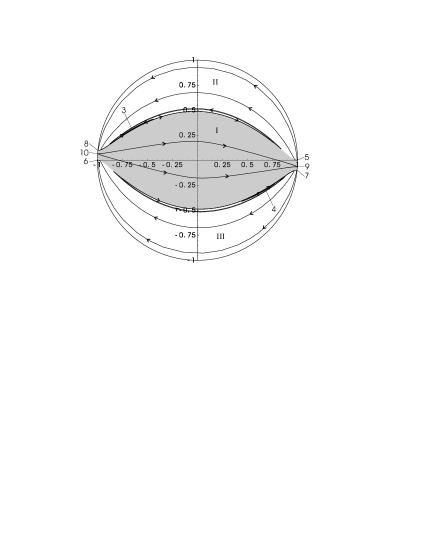
Figure 2: Phase plane of cosmological solutions for $\omega=0$ and $\delta=0.1$.

Figure 2 is seen to be split into three separate regions labelled I, II and III. The boundaries between these regions are the sub-manifolds $R=0$. As pointed out by Carloni et. al. the plane $R=0$ is an invariant sub-manifold of the phase space through which trajectories cannot pass.

The equation for $R$ in a FRW universe, (14), can now be rewritten as

$$R=\frac{16\pi\rho}{\delta R^{\delta}}((1+\delta)y^{2}+\delta(1+\delta)xy-1).$$ (34)

This shows that the boundary $R=0$ is given in terms of $x$ and $y$ by $(1+\delta)y^{2}+\delta(1+\delta)xy-1=0$ and that in region I the sign of $R$ must be opposite to the sign of $\delta$ in order to have a positive $\rho$. Similarly, in regions II and III, $R$ must have the same sign as $\delta$ in order to ensure a positive $\rho$.

It can be seen that regions II and III are symmetric under a rotation of $\pi$ and a reversal of the direction of the trajectories. As region II is exclusively in the semi–circle $y\geqslant 0$ all trajectories confined to this region correspond to eternally expanding (or expanding and asymptotically static) universes. Similarly, region III is confined to the semi–circle $y\leqslant 0$ and so all trajectories confined to this region correspond to eternally contracting (or contracting and asymptotically static) universes. Region I, however, spans the $y=0$ plane and so can have trajectories which correspond to universes with both expanding and contracting phases. In fact, it can be seen from figure 2 that, for $\delta=0.1$ all trajectories in region I are initially expanding and eventually contracting.

It can be seen from figure 2 that in region I the only stable attractors are, at early times, the expanding point 10 and at late times the contracting point 9. (By ‘attractors at early times’ we mean the critical points which are approached if the trajectories are followed backwards in time). Both of these points correspond to the solution

$$a\propto t^{\delta\frac{(1+2\delta)}{(1-\delta)}}$$

which describes a slow evolution independent of the matter content of the universe. Notably, region I only has stable attractor points, at both early and late times, which have been shown to correspond to $t\rightarrow$constant; region I therefore does not have an asymptotic attractor when $t\rightarrow\infty$, for the range of $\delta$ being considered. In region II the only stable attractors can be seen to be the static point 5 at some early finite time, $t_{0}$, and the expanding matter-driven expansion described by point 3 as $t\rightarrow\infty$. Conversely, in region III the only stable attractors are the contracting point 4 for $t\rightarrow-\infty$ and the static point 6 for $t\rightarrow t_{0}$.

Figure 3 shows the compactified phase plane for a universe containing pressureless dust and having $\delta=-0.1$.

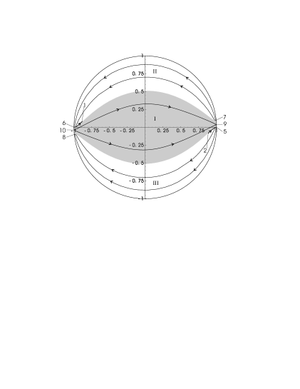
Figure 3: Phase plane of cosmological solutions for $\omega=0$ and $\delta=-0.1$.

Figure 3 is split into three separate regions in a similar way to figure 2, with the boundary between the regions again corresponding to $R=0$ and is given in terms of $x$ and $y$ by (34). Regions II and III again correspond to expanding and contacting solutions, respectively. Region I, still has point 10 as the early-time attractor and point 9 as the late-time attractor, but now has all trajectories initially contracting and eventually expanding. There are still no stable attractors in Region I which correspond to regions where $t\rightarrow\infty$. Region II now has point 7 as an early-time stable attractor solution and point 1 as a late-time stable attractor solution, corresponding to $a\rightarrow t^{\frac{1}{2}}$ as $t\rightarrow\infty$. Point 3, which was the stable attractor at late times when $\delta=0.1$ is now no longer located in Region II and can instead be located in region I where it is now a saddle-point in the phase plane. Interestingly, the value of $\delta$ for which point 3 ceases to behave as a stable attractor ($\delta=0$) is exactly the same value of $\delta$ at which the point moves from region II into region I; so as long as point 3 can be located in region I, it is the late-time stable attractor solution and as soon as it moves into region I it becomes a saddle-point. At this same value of $\delta,$ point 1 ceases to be a saddle-point and becomes the late-time stable attractor for region II, so that region II always has a stable late-time attractor where $t\rightarrow\infty$. Region III behaves in a similar way to the description given for region II above, under a rotation of $\pi$ and with the directions of the trajectories reversed.

Phase planes diagrams for $\omega=0$ with values of $\delta$ other than $0.1$ and $-0.1$, but still within the range

$$-\frac{\sqrt{73+66\omega+9\omega^{2}}+3(1+\omega)}{4(4+3\omega)}<\delta<\frac{\sqrt{73+66\omega+9\omega^{2}}-3(1+\omega)}{4(4+3\omega)},$$

look qualitatively similar to those above with some of the attractor properties of the critical points being exchanged as they pass each other. Notably, for $\delta<-\frac{1}{4}$ point 3 returns to region II and once again becomes the stable late-time attractor for trajectories in that region. The points that are the stable attractors for any particular value of $\delta$ can be read off from the tables in the previous section.

Universes filled with perfect fluid black-body radiation also retain qualitatively similar phase-plane diagrams to the ones above; with the notable difference that the point 3 is always located in region II and is always the late-time stable attractor of that region. This can be seen directly from the Ricci scalar for the solution (15) which is given by

$$R=\frac{3\delta(1+\delta)}{t^{2}}$$

and can be seen to have the same sign as $\delta$, for $\delta>-1$, and so is always found in region II.

For a spatially-flat, expanding FRW universe containing black-body radiation we therefore have that (15) is the generic attractor as $t\rightarrow\infty$. Similarly, for a spatially-flat, expanding, matter-dominated FRW universe (15) is the attractor solution as $t\rightarrow\infty$; except when $-\frac{1}{4}<\delta<0$, in which case it is point 1 ($a\propto t^{\frac{1}{2}}$).

If we require a stable period of matter domination, during which $a(t)\sim t^{\frac{2}{3}}$, we therefore have the theoretical constraint $\delta>0$ (or $\delta<-\frac{1}{4}$). Such a period is necessary for structure to form through gravitational collapse in the post-recombination era of the universe’s expansion.

The effect of a non–zero curvature, $\kappa\neq 0$, on the cosmological dynamics is similar to the general relativistic case. The role of negative curvature ($\kappa=-1$) can be deduced by noting that its effect is similar to that of a fluid with $\omega=-1/3$. The solution (15) is unstable to any perturbation away from flatness and will diverge away from $\kappa=0$ as $t\rightarrow\infty$. This is usually referred to as the ‘flatness problem’ and can be seen to exist in this theory from the analysis of Carloni et. al. Car04 .

III.2 Physical consequences

The modified cosmological dynamics discussed in the last section lead to different predictions for the outcomes of physical processes, such as primordial nucleosynthesis and CMB formation, compared to the standard general-relativistic model. The relevant modifications to these physical processes, and the bounds that they can impose upon the theory, will be discussed in this section. We will use the solutions (15) as they have been shown to be the generic attractors as $t\rightarrow\infty$ (except for the case $-\frac{1}{4}<\delta<0$ when $\omega=0$, which has been excluded as physically unrealistic on the grounds of structure formation).

III.2.1 Primordial nucleosynthesis

We find that the temperature-time adiabat during radiation domination for the solution (15) is given by the exact relation

$$t^{2(1+d)}=\frac{A}{T^{4}}$$ (35)

where, as usual (with units $\hbar=c=1=k_{B}$),

$$\rho=\frac{g\pi^{2}}{15}T^{4}$$

where $g$ is the total number of relativistic spin states at temperature $T$. The constant $A$ can be determined from the generalised Friedmann equation (13) and is dependent on the present day value of the Ricci scalar, through equation (10). (This dependence is analogous to the dependence of scalar–tensor theories on the evolution of the non–minimally coupled scalar, as may be expected from the relationship between these theories Mag94 ). As a first approximation we assume the universe to have been matter dominated throughout its later history; this allows us to write

$$A=\left(\frac{45(1-2\delta)(1-2\delta-5\delta^{2})}{32(1-\delta)g\pi^{3}G}\right)\left(\frac{2(1+\delta)}{3H_{0}}\right)^{2\delta}$$ (36)

where $H_{0}$ is the value of Hubble’s constant today and we have used the solution (15) to model the evolution of $a(t)$. Adding a recent period of accelerated expansion will refine the constant $A$, but in the interests of brevity we exclude this from the current analysis.

As usual, the weak-interaction time is given by

$$t_{wk}\propto\frac{1}{T^{5}}.$$

The freeze–out temperature, $T_{f}$, for neutron–proton kinetic equilibrium is then defined by

$$t(T_{f})=t_{wk}(T_{f}),$$

hence the freeze–out temperature in this theory, with $\delta\neq 0$, is related to that in the general-relativistic case with $\delta=0$, $T_{f}^{GR}$, by

$$T_{f}=C(T_{f}^{GR})^{\frac{3(1+\delta)}{(3+5\delta)}}$$ (37)

where

$$C=\left(\frac{(1-\delta)}{(1-2\delta)(1-2\delta-5\delta^{2})}\right)^{\frac{1}{2(2+5\delta)}}\left(\frac{45}{32g\pi^{3}G}\right)^{\frac{\delta(1+\delta)}{2(3+5\delta)}}\left(\frac{3H_{0}}{2(1+\delta)}\right)^{\frac{\delta}{(3+5\delta}}.$$ (38)

The neutron–proton ratio, $n/p$, is now determined at temperature $T$ when the equilibrium holds by

$$\frac{n}{p}=\exp\left(-\frac{\Delta m}{T}\right).$$

where $\Delta m$ is the neutron-proton mass difference. Hence the neutron–proton ratio at freeze-out in the $R^{1+\delta}$ early universe is given by

$$\frac{n}{p}=\exp\left(-\frac{\Delta m}{C(T_{f}^{GR})^{1-\varepsilon}}\right),$$

where

$$\varepsilon\equiv\frac{2\delta}{3+5\delta}.$$

The frozen–out $n/p$ ratio in the $R^{1+\delta}$ theory is given by a power of its value in the general relativistic case, $\left(\frac{n}{p}\right)_{GR}\approx 1/7$, by

$$\frac{n}{p}=\left(\frac{n}{p}\right)_{GR}^{C(T_{f}^{GR})^{\varepsilon}}.$$

It is seen that when $C(T_{f}^{GR})^{\varepsilon}>1$ ($\delta<0$) there is a smaller frozen-out neutron-proton ratio that in the general-relativistic case and consequently a lower final helium-4 abundance than in the standard general-relativistic early universe containing the same number of relativistic spin states. This happens because the freeze-out temperature is lower than in general relativity. The neutrons remain in equilibrium to a lower temperature and their slightly higher mass shifts the number balance more towards the protons the longer they are in equilibrium. Note that a reduction in the helium-4 abundance compared to the standard model of general relativity is both astrophysically interesting and difficult to achieve (all other variants like extra particle species shv ; nus , anisotropies ht ; jb1 ; jb2 ; jb3 , magnetic fields mag ; YM , gravitational waves jb1 ; jb2 ; skew , or varying $G$ bmaeda ; newt ; clift , lead to an increase in the expansion rate and in the final helium-4 abundance). Conversely, when $C(T_{f}^{GR})^{\varepsilon}<1$ ($\delta>0$) freeze-out occurs at a higher temperature than in general relativity and a higher final helium-4 abundance fraction results. The final helium-4 mass fraction $Y$ is well approximated by

$$Y=\frac{2n/p}{(1+n/p)}.$$ (39)

It is now possible to constrain the value of $\delta$ using observational abundances of the light elements. In doing this we will use the results of Carroll and Kaplinghat Car02 who consider nucleosynthesis with a Hubble constant parametrised by

$$H(T)=\left(\frac{T}{1MeV}\right)^{\alpha}H_{1}.$$

Our theory can be cast into this form by substituting

$$\alpha=\frac{2}{(1+\delta)}$$

and

$$H_{1}=\frac{(1+\delta)}{2}A^{-\frac{1}{2(1+\delta)}}(1MeV)^{\frac{2}{(1+\delta)}},$$

so, taking $g=43/8$, $G=6.72\times 10^{-45}MeV^{-2}$ and $H_{0}=1.51\times 10^{-39}MeV$ Ben03 , this can be rewritten as

$$H_{1}=\frac{(1+\delta)}{2}\left(\frac{7.96\times 10^{-43}(1-\delta)}{(1-2\delta)(1-2\delta-5\delta^{2})}\right)^{\frac{1}{2(1+\delta)}}\left(\frac{2.23\times 10^{-39}}{(1+\delta)}\right)^{\frac{\delta}{(1+\delta)}}MeV.$$

Carroll and Kaplinghat use the observational abundances inferred by Olive et. al. Oli00

$$0.228\leqslant Y_{P} \leqslant 0.248$$

$$2\leqslant 10^{5}\times \frac{D}{H}\leqslant 5$$

$$1\leqslant 10^{10}\times \frac{{}^{7}Li}{H}\leqslant 3$$

to impose the constraint

$$H_{1}=H_{c}\left(\frac{T_{c}}{MeV}\right)^{-\alpha}$$

where $H_{c}=2.6\pm 0.9\times 10^{-23}MeV$ at $T_{c}=0.2MeV$ for $0.5\leqslant\eta_{10}\leqslant 50$, or $H_{c}=2.0\pm 0.3\times 10^{-23}$ for $1\leqslant\eta_{10}\leqslant 10$ and $\eta_{10}$ is $10^{10}$ times the baryon to photon ratio.

These results can now be used to impose upon $\delta$ the constraints

$$-0.017\leqslant\delta\leqslant 0.0012,$$

for $0.5\leqslant\eta_{10}\leqslant 50$, or

$$-0.0064\leqslant\delta\leqslant 0.0012,$$ (40)

for $1\leqslant\eta_{10}\leqslant 10$.

III.2.2 Horizon size at matter–radiation equality

The horizon size at the epoch of matter–radiation equality is of great observational significance. During radiation domination cosmological perturbations on sub–horizon scales are effectively frozen. Once matter domination commences, however, perturbations on all scales are allowed to grow and structure formation begins. The horizon size at matter–radiation equality is therefore frozen into the power spectrum of perturbations and is observable. Calculation of the horizon sizes in this theory proceeds in a similar way to that in Brans–Dicke theory Lid98 .

In making an estimate of the horizon sizes in $R^{1+\delta}$ theory we will use the generalised Friedmann equation, (13), in the form

$$H^{2}+\delta H\frac{\dot{R}}{R}-\frac{\delta R}{6(1+\delta)}=\frac{8\pi G(1-\delta)}{3(1-2\delta)}\frac{R_{0}^{\delta}}{R^{\delta}}\rho.$$ (41)

Again, we assume the form (15) to model the evolution of the scale factor during the epoch of matter domination. This gives the results

$$a(t) =a_{0}\left(\frac{t}{t_{0}}\right)^{\frac{2(1+\delta)}{3}}$$

$$H_{0} =\frac{2(1+\delta)}{3t_{0}}$$

$$\rho_{m} =\frac{3H_{0}^{2}}{16\pi G}\frac{(1-2\delta)(2-3\delta-8\delta^{2})}{(1-\delta)(1+\delta)^{2}}\frac{a_{0}^{3}}{a^{3}}$$

$$R(t) =\frac{4(1+5\delta+4\delta^{2})}{3t^{2}}$$

during the matter-dominated era. In order to simplify matters we assume the above solutions to hold exactly from the time of matter–radiation equality up until the present (neglecting the small residual radiation effects and the very late time acceleration). Substituting them into (41) along with $\rho_{eq}=2\rho_{meq}$ at equality we can then solve for $H_{eq}$ to first order in $\delta$ to find

$$\frac{a_{eq}H_{eq}}{a_{0}H_{0}}\simeq\sqrt{2}\sqrt{1+z_{eq}}^{\frac{1-2\delta}{1+\delta}}(1-2.686\delta)+O(\delta^{2})$$ (42)

where $z_{eq}$ is the redshift at matter radiation equality and $H$ has been treated as an independent parameter. The value of $1+z_{eq}$ can now be calculated in this theory as

$$1+z_{eq}=\frac{\rho_{r0}}{\rho_{m0}}.$$ (43)

Taking the present day temperature of the of the microwave background as $T=2.728\pm 0.004K$ Fix96 gives

$$\rho_{r0}=3.37\times 10^{-39}MeV^{4}$$ (44)

where three families of light neutrinos have been assumed at a temperature lower than that of the microwave background by a factor $(4/11)^{\frac{1}{3}}$. Using the same values for $G$ and $H_{0}$ as above we than find from the above expression for $\rho_{m}$ that

$$\rho_{m0}=2.03\times 10^{-35}\frac{(1-2\delta)(2-3\delta-8\delta^{2})}{(1-\delta)(1+\delta)^{2}}MeV^{4}.$$ (45)

Substituting (44), (45) and (43) into (42) then gives the expression for the horizon size at equality, to first order in $\delta$, as

$$\frac{a_{eq}H_{eq}}{a_{0}H_{0}}\simeq 155(1-19\delta)+O(\delta^{2}).$$ (46)

This expression shows that the horizon size at matter–radiation equality will be shifted by $\sim 1\%$ for a value of $\delta\sim 0.0005$. This shift in horizon size should be observable in a shift of the peak of the power spectrum of perturbations, compared to its position in the standard general relativistic cosmology. Microwave background observations, therefore, allow a potentially tight bound to be derived on the value of $\delta$. This effect is analogous to the shift of power–spectrum peaks in Brans–Dicke theory (see e.g. Lid98 , Che99 ).

A full analysis of the spectrum of perturbations in this theory requires a knowledge of the evolution of linearised perturbations as well as a marginalization over other parameters which can mimic this effect (e.g. baryon density). Such a study is beyond the scope of the present work.

IV Static and spherically–symmetric solutions

In order to test the $R^{n}$ gravity theory in the weak-field limit by means of the standard solar-system tests of general relativity we need to find the analogue of the Schwarzschild metric in this generalised theory and use it to describe the gravitational field of the Sun. In the absence of any matter the field equations (2) can be written as

$$R_{ab}=\delta\left(\frac{R_{;}^{\ cd}}{R}-(1-\delta)\frac{R_{,}^{\ c}R_{,}^{\ d}}{R^{2}}\right)\left(g_{ac}g_{bd}+\frac{1}{2}\frac{(1+2\delta)}{(1-\delta)}g_{ab}g_{cd}\right).$$ (47)

We find that an exact static spherically symmetric solution of these field equations is given in Schwarzschild coordinates by the line–element

$$ds^{2}=-A(r)dt^{2}+\frac{dr^{2}}{B(r)}+r^{2}(d\theta^{2}+\sin^{2}\theta d\phi^{2})$$ (48)

where

$$A(r) =r^{2\delta\frac{(1+2\delta)}{(1-\delta)}}+\frac{C}{r^{\frac{(1-4\delta)}{(1-\delta)}}}$$

$$B(r) =\frac{(1-\delta)^{2}}{(1-2\delta+4\delta^{2})(1-2\delta(1+\delta))}\left(1+\frac{C}{r^{\frac{(1-2\delta+4\delta^{2})}{(1-\delta)}}}\right)$$

and $C=$ constant. This solution is conformally related to the $Q=0$ limit of the one found by Chan, Horne and Mann for a static spherically–symmetric space–time containing a scalar–field in a Liouville potential Cha95 . It reduces to Schwarzschild in the limit of general relativity: $\delta\rightarrow 0$.

In order to evaluate whether or not this solution is physically relevant we will proceed as follows. A dynamical systems approach will be used to establish the asymptotic attractor solutions of the field equations (47). The field equations will then be perturbed around these asymptotic attractor solutions and solved to first order in the perturbed quantities. This linearised solution will then be treated as the physically relevant static and spherically–symmetric weak–field limit of the field equations (47) and compared with the exact solution (48).

IV.1 Dynamical system

The dynamical systems approach has already been applied to a situation of this kind by Mignemi and Wiltshire Mig89 . We present a brief summary of the relevant points of their work in the above notation; for a comprehensive analysis the reader is referred to their paper.

Taking the value of sign$(R)$ from (48) as sign$(-\delta(1+\delta)/(1-2\delta(1+\delta)))$ and making a suitable choice of $\Omega_{0}$ allows the scalar-field potential (4) to be written as

$$V(\phi)=-\frac{3\delta^{2}}{8\pi G(1-2\delta(1+\delta))}\exp\left({\sqrt{\frac{16\pi G}{3}}\frac{(1-\delta)}{\delta}\phi}\right).$$ (49)

In four dimensions Mignemi and Wiltshire’s choice of line–element corresponds to

$$d\bar{s}^{2}=e^{2U(\xi)}\left(-dt^{2}+\bar{r}^{4}(\xi)d\xi^{2}\right)+\bar{r}^{2}(\xi)(d\theta^{2}+\sin^{2}\theta d\phi^{2})$$ (50)

which, after some manipulation, gives the field equations (3) as

$$\zeta^{\prime\prime} =-\frac{2c_{1}^{2}(1-\delta)^{2}+6\delta^{2}\eta^{\prime}{}^{2}-24\delta^{2}\eta^{\prime}\zeta^{\prime}-2(1-2\delta-8\delta^{2})\zeta^{\prime}{}^{2}}{1-2\delta+4\delta^{2}}-e^{2\zeta}$$ (51)

$$\eta^{\prime\prime} =\frac{(1-2\delta-8\delta^{2})(c_{1}^{2}(1-\delta)^{2}+3\delta^{2}\eta^{\prime}{}^{2}-12\delta^{2}\eta^{\prime}\zeta^{\prime}-(1-2\delta-8\delta^{2})\zeta^{\prime}{}^{2})}{3\delta^{2}(1-2\delta+4\delta^{2})}+\frac{(1-2\delta(1+\delta))}{3\delta^{2}}e^{2\zeta}$$ (52)

and

$$e^{2\eta}=-\frac{(1-2\delta(1+\delta))}{3\delta^{2}(1-2\delta+4\delta^{2})}\left(c_{1}^{2}(1-\delta)^{2}+3\delta^{2}\eta^{\prime}{}^{2}-12\delta^{2}\eta^{\prime}\zeta^{\prime}-(1-2\delta-8\delta^{2})\zeta^{\prime}{}^{2}+(1-2\delta+4\delta^{2})e^{2\zeta}\right)$$ (53)

where

$$\zeta(\xi) =U(\xi)+\log\bar{r}(\xi)$$

$$\eta(\xi) =-\frac{(1-2\delta(1+\delta))}{3\delta^{2}}U(\xi)+2\log\bar{r}(\xi)-\frac{(1-\delta)^{2}}{3\delta^{2}}c_{1}\xi+\text{constant.}$$

Primes denote differentiation with respect to $\xi$ and $c_{1}$ is a constant of integration.

Defining the variables $X$, $Y$ and $Z$ by

$$X=\zeta^{\prime}\qquad Y=\eta^{\prime}\qquad Z=e^{\zeta}$$

the field equations (51) and (52) can then be written as the following set of first-order autonomous differential equations

$$X^{\prime} =-\frac{2c_{1}^{2}(1-\delta)^{2}+6\delta^{2}Y^{2}-24\delta^{2}XY-2(1-2\delta-8\delta^{2})X^{2}}{1-2\delta+4\delta^{2}}-Z^{2}$$ (54)

$$Y^{\prime} =\frac{(1-2\delta-8\delta^{2})(c_{1}^{2}(1-\delta)^{2}+3\delta^{2}Y^{2}-12\delta^{2}XY-(1-2\delta-8\delta^{2})X^{2})}{3\delta^{2}(1-2\delta+4\delta^{2})}+\frac{(1-2\delta(1+\delta))}{3\delta^{2}}Z^{2}$$ (55)

$$Z^{\prime} =XZ.$$ (56)

(The reader should note the different definition of $Z$ here to that of Mignemi and Wiltshire). As identified by Mignemi and Wiltshire, the only critical points at finite values of $X$, $Y$ and $Z$ are in the plane $Z=0$ along the curve defined by

$$c_{1}^{2}(1-\delta)^{2}+3\delta^{2}Y^{2}-12\delta^{2}XY-(1-2\delta-8\delta^{2})X^{2}=0.$$

These curves are shown as bold lines in figure 4, together with some sample trajectories from equations (54)and (55). From the definition above we see that the condition $Z=0$ is equivalent to $\bar{r}e^{U}=0$. Whilst we do not consider trajectories confined to this plane to be physically relevant we do consider the plot to be instructive as it gives a picture of the behaviour of trajectories close to this surface and displays the attractive or repulsive behaviour of the critical points, which can be the end points for trajectories which could be considered as physically meaningful.

Figure 4: The $Z=0$ plane of the phase space defined by $X$,$Y$ and $Z$ for $\delta=0.1$ and $c_{1}=0.5$. The bold lines show the critical points in this plane and the diagonal lines show the unphysical trajectories confined to this plane. The dotted line is $Y=2X$ and separates the critical points where $\xi\rightarrow\infty$ from the points where $\xi\rightarrow-\infty$

The dotted line in figure 4 corresponds to the line $Y=2X$ and separates two different types of critical points. The critical points with $Y>2X$ can be seen to be repulsive to the trajectories in the $Z=0$ plane and correspond to the limit $\xi\rightarrow-\infty$. Conversely, the points with $Y<2X$ are attractive and correspond to the limit $\xi\rightarrow\infty$. As $Z=\bar{r}e^{U},$ all critical points of this type in the $Z=0$ plane correspond either to naked singularities, $\bar{r}\rightarrow 0$, or regular horizons, $\bar{r}\rightarrow$constant.

The two bold lines in figure 4 are the points at which the surface defined by

$$c_{1}^{2}(1-\delta)^{2}+3\delta^{2}Y^{2}-12\delta^{2}XY-(1-2\delta-8\delta^{2})X^{2}+(1-2\delta+4\delta^{2})Z^{2}=0$$

crosses the $Z=0$ plane. This surface splits the phase space into three separate regions between which trajectories cannot move. These regions are labelled $I$, $II$ and $III$ in figure 4. It can be seen from (53) that trajectories are confined to either regions $I$ or $II$, for the potential defined by (49). If we had chosen the opposite value of sign$(R)$ in (4) then trajectories would be confined to region $III$. We will show, however, that region $III$ does not contain solutions with asymptotic regions in which $\bar{r}\rightarrow\infty$ and so is of limited interest for our purposes.

In order to find the remaining critical points it is necessary to analyse the sphere at infinity. This can be done by making the transformation

$$X=\rho\sin\theta\cos\phi\qquad Y=\rho\sin\theta\sin\phi\qquad Z=\rho\cos\theta$$

and taking the limit $\rho\rightarrow\infty$. The set of equations (54), (55) and (56) then give

$$\frac{d\theta}{d\tau}\rightarrow-\frac{\cos\theta}{24\delta^{2}(1-2\delta+4\delta)}(6\delta^{2}\cos\phi(3-3\delta(2-9\delta)+(1-\delta(2+11\delta))\cos 2\theta)\\ -(3-3\delta(4-\delta(15-22\delta-32\delta^{2}))+(5-\delta(20-\delta(3+34\delta+32\delta^{2})))\cos 2\theta)\sin\phi\\ -2(18\delta^{2}(1-\delta(2+7\delta))\cos 3\phi-(1-\delta(4+\delta(9-26\delta+32\delta^{2})))\sin 3\phi)\sin^{2}\theta)$$

and

$$\frac{d\phi}{d\tau}\rightarrow-\frac{1}{24\delta^{2}(1-2\delta+4\delta^{2})}(6\delta^{2}(1-\delta(2+41\delta)-5(1-\delta(2+5\delta))\cos 2\theta)\text{cosec}\theta\sin\phi\\ +2((1-\delta(4+\delta(9-26\delta+32\delta^{2})))\cos 3\phi+18\delta^{2}(1-\delta(2+7\delta))\sin 3\phi)\sin\theta\\ -2\cos\phi(4(1-2\delta(2-\delta(3-2\delta-4\delta^{2})))\text{cosec}\theta-(7-\delta(28+\delta(15-2\delta(43+128\delta))))\sin\theta))$$

where $d\tau=\rho d\xi$. These equations can be used to plot the positions of critical points and trajectories on the sphere at infinity. The result of this is shown in figure 5. Once again, these trajectories do not correspond to physical solutions in the phase space but are illustrative of trajectories at large distances and help to show the attractive or repulsive nature of the critical points.

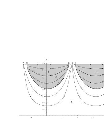
Figure 5: The surface at infinity of the phase space defined by $X$,$Y$ and $Z$ for $\delta=0.1$. The shaded areas show where regions $I$ and $II$. Region $III$ is unshaded.

The surface at infinity has eight critical points, labelled $A$-$H$ in figure 5. Points $A$ and $B$ are the end-points of the trajectory that goes through the origin in figure 4 and are located at

$$\theta=\frac{\pi}{2},\qquad\text{and}\qquad\phi_{1,(2)}=\cos^{-1}\left(\frac{-6\delta^{2}}{\sqrt{1-4\delta-12\delta^{2}+32\delta^{3}+100\delta^{4}}}\right)(+\pi)$$

or, in terms of the original functions in the metric (50),

$$\bar{r}\rightarrow(\xi-\xi_{1})^{\frac{3\delta^{2}}{(1-2\delta-8\delta^{2})}}\qquad\text{and}\qquad e^{U}\rightarrow(\xi-\xi_{1})^{\frac{3\delta^{2}}{(1-2\delta-8\delta^{2})}},$$

where $\xi_{1}$ is a constant of integration. The points $A$ and $B$ therefore both correspond to $\xi\rightarrow\xi_{1}$ and hence to $\bar{r}\rightarrow 0$.

Points $C$, $D$, $E$ and $F$ are the four end points of the two curves in figure 4 and therefore correspond to $\xi\rightarrow\infty$ or $-\infty$ and $\bar{r}\rightarrow 0$ or constant.

The remaining points, $G$ and $H$, are located at

$$\phi_{1,(2)}=\frac{\pi}{4}(+\pi)\qquad\text{and}\qquad\theta=\frac{1}{2}\cos^{-1}\left(-\frac{1-2\delta+10\delta^{2}}{3-6\delta+6\delta^{2}}\right)$$

or

$$\bar{r}^{\frac{(1-2\delta+4\delta^{2})}{(1-\delta)^{2}}}\rightarrow\pm\sqrt{\frac{(1-2\delta-2\delta^{2})}{(1-2\delta+4\delta^{2})}}\frac{1}{(\xi-\xi_{2})}\qquad\text{and}\qquad e^{\frac{(1-2\delta+4\delta^{2})U}{3\delta^{2}}}\rightarrow\pm\sqrt{\frac{(1-2\delta-2\delta^{2})}{(1-2\delta+4\delta^{2})}}\frac{1}{(\xi-\xi_{2})},$$ (57)

where $\xi_{2}$ is an integration constant, the positive branch corresponds to point $H$ and the negative branch to point $G$. These points are, therefore, the asymptotic limit of the exact solution (48) and correspond to $\xi\rightarrow\xi_{2}$ and hence $\bar{r}\rightarrow\infty$.

Whilst it may initially appear that trajectories are repelled from the point $H$, this is only the case in terms of the coordinate $\xi$. In terms of the more physically relevant quantity $\bar{r},$ the point $H$ is an attractor. This can be seen from the first equation in (57). Taking the positive branch here it can be seen that $\bar{r}$ increases as $\xi$ decreases. So, in terms of $\bar{r}$ the points $G$ and $H$ are both attractors, as $\bar{r}\rightarrow\infty$.

We can now see that in region $I$ all trajectories appear to start at critical points corresponding to either $\bar{r}\rightarrow 0$ or constant and end at point $G$ where $\bar{r}\rightarrow\infty$. Region $II$ appears to share the same features as region $I$ with all trajectories starting at either $\bar{r}\rightarrow 0$ or constant and ending at $H$ where $\bar{r}\rightarrow\infty$. Region $III$ has no critical points corresponding to $\bar{r}\rightarrow\infty$ and so all trajectories both begin and end on points corresponding to $\bar{r}\rightarrow 0$ or constant.

Therefore the only solutions with an asymptotic region in which $\bar{r}\rightarrow\infty$ exist in regions $I$ and $II$ where the potential can be described by equation (49). Furthermore, all trajectories in regions $I$ and $II$ appear to be attracted to the solution

$$ds^{2}=-\bar{r}^{\frac{6\delta^{2}}{(1-\delta)^{2}}}dt^{2}+\frac{(1-2\delta+4\delta^{2})(1-2\delta-2\delta^{2})}{(1-\delta)^{4}}d\bar{r}^{2}+\bar{r}^{2}(d\theta^{2}+\sin^{2}\theta d\phi^{2}),$$ (58)

which is the asymptotic behaviour of the solution found by Chan, Horne and Mann Cha95 . We therefore conclude that all solutions with an asymptotic region in which $\bar{r}\rightarrow\infty$ are attracted towards the solution (58) as $\bar{r}\rightarrow\infty$.

Rescaling the metric back to the original conformal frame we therefore conclude that the generic asymptotic attractor solution to the field equations, (47), is

$$ds^{2}=-r^{2\delta\frac{(1+2\delta)}{(1-\delta)}}dt^{2}+\frac{(1-2\delta+4\delta^{2})(1-2\delta-2\delta^{2})}{(1-\delta)^{2}}dr^{2}+r^{2}(d\theta^{2}+\sin^{2}\theta d\phi^{2})$$ (59)

as $r\rightarrow\infty$. It reduces to Minkowski in the $\delta\rightarrow 0$ limit of general relativity.

IV.2 Linearised solution

We now proceed to find the general solution, to first order in perturbations, around the background described by (59). Writing the perturbed line-element as

$$ds^{2}=-r^{2\delta\frac{(1+2\delta)}{(1-\delta)}}(1+V(r))dt^{2}+\frac{(1-2\delta+4\delta^{2})(1-2\delta-2\delta^{2})}{(1-\delta)^{2}}(1+W(r))dr^{2}+r^{2}(d\theta^{2}+\sin^{2}\theta d\phi^{2})$$ (60)

and making no assumptions about the order of $R$ the field equations (47) become, up to first order in $V$ and $W$,

$$\frac{\delta(1+2\delta)(1+2\delta^{2})}{(1-\delta)^{2}r^{2}}+\frac{(1+2\delta^{2})}{(1-\delta)}\frac{V^{\prime}}{r}-\frac{\delta(1-2\delta)}{2(1-\delta)}\frac{W^{\prime}}{r}+\frac{V^{\prime\prime}}{2}\\ =\frac{\delta(1+2\delta)}{2}\frac{R^{\prime}{}^{2}}{R^{2}}-\frac{\delta(1+2\delta)}{2(1-\delta)}\frac{R^{\prime\prime}}{R}-\frac{3\delta}{4(1-\delta)}\frac{R^{\prime}}{R}V^{\prime}-\frac{\delta(1+2\delta)(2+\delta)}{2(1-\delta)^{2}r}\frac{R^{\prime}}{R}+\frac{\delta(1+2\delta)}{4(1-\delta)}\frac{R^{\prime}}{R}W^{\prime},$$ (61)

$$\frac{\delta(1+2\delta)(1-2\delta-2\delta^{2})}{(1-\delta)^{2}r^{2}}-\frac{\delta(1+2\delta)}{(1-\delta)}\frac{V^{\prime}}{r}+\frac{(2-\delta+2\delta^{2})}{2(1-\delta)}\frac{W^{\prime}}{r}-\frac{V^{\prime\prime}}{2}\\ =-\frac{3\delta}{2}\frac{R^{\prime}{}^{2}}{R^{2}}+\frac{3\delta}{2(1-\delta)}\frac{R^{\prime\prime}}{R}+\frac{\delta(1+2\delta)(2-\delta+2\delta^{2})}{2(1-\delta)^{2}r}\frac{R^{\prime}}{R}+\frac{\delta(1+2\delta)}{4(1-\delta)}\frac{R^{\prime}}{R}V^{\prime}-\frac{3\delta}{4(1-\delta)}\frac{R^{\prime}}{R}W^{\prime}$$ (62)

and

$$-\frac{2\delta(3-4\delta+2\delta^{2}+8\delta^{3})}{(1-\delta)^{2}r^{2}}+\frac{2(1-2\delta+4\delta^{2})(1-2\delta-2\delta^{2})}{(1-\delta)^{2}r^{2}}W-\frac{V^{\prime}}{r}+\frac{W^{\prime}}{r}\\ =-\delta(1+2\delta)\frac{R^{\prime}{}^{2}}{R^{2}}+\frac{\delta(1+2\delta)}{(1-\delta)}\frac{R^{\prime\prime}}{R}+\frac{\delta(4-\delta+2\delta^{2}+4\delta^{3})}{(1-\delta)^{2}r}\frac{R^{\prime}}{R}+\frac{\delta(1+2\delta)}{2(1-\delta)}\frac{R^{\prime}}{R}V^{\prime}-\frac{\delta(1+2\delta)}{2(1-\delta)}\frac{R^{\prime}}{R}W^{\prime}.$$ (63)

Expanding $R$ to first order in $V$ and $W$ gives

$$R=-\frac{6\delta(1+\delta)}{(1-2\delta-2\delta^{2})}\frac{1}{r^{2}}+R_{1}$$ (64)

where

$$R_{1}=\frac{2(1+\delta+\delta^{2})}{(1-2\delta-2\delta^{2})}\frac{W}{r^{2}}-\frac{2(1-\delta)(1+2\delta^{2})}{(1-2\delta-2\delta^{2})(1-2\delta+4\delta^{2})}\frac{V^{\prime}}{r}\\ +\frac{(1-\delta)(2-\delta+2\delta^{2})}{(1-2\delta-2\delta^{2})(1-2\delta+4\delta^{2})}\frac{W^{\prime}}{r}-\frac{(1-\delta)^{2}}{(1-2\delta-2\delta^{2})(1-2\delta+4\delta^{2})}V^{\prime\prime}.$$ (65)

Substituting (64) into the field equations (61), (62) and (63) and eliminating $R_{1}$ using (65) leaves

$$\frac{(1+\delta+\delta^{2})(5-12\delta+12\delta^{2}+4\delta^{3})}{3(1-\delta)^{2}(1+\delta)}\frac{W}{r}+\frac{(16-47\delta+76\delta^{2}-34\delta^{3}-16\delta^{4}+32\delta^{5})}{6(1-\delta^{2})(1-2\delta+4\delta^{2})}W^{\prime}\\ -\frac{(1+\delta+7\delta^{2}-19\delta^{3}+44\delta^{4}+20\delta^{5})}{3(1-\delta^{2})(1-2\delta+4\delta^{2})}\frac{Y}{r}-\frac{(8-15\delta+18\delta^{2}+16\delta^{3})}{6(1+\delta)(1-2\delta+4\delta^{2})}Y^{\prime}\\ =-\frac{(1-2\delta-2\delta^{2})(5-12\delta+12\delta^{2}+4\delta^{3})}{12(1-\delta^{2})(1+\delta)}\frac{\psi}{r}-\frac{(1-2\delta-2\delta^{2})}{4(1-\delta^{2})}\psi^{\prime},$$

$$-\frac{(1+2\delta)(1+\delta+\delta^{2})(3-4\delta+4\delta^{2})}{3(1-\delta)^{2}(1+\delta)}\frac{W}{r}-\frac{(1+2\delta)(2-\delta+2\delta^{2})(3-4\delta+4\delta^{2})}{6(1-\delta^{2})(1-2\delta+4\delta^{2})}W^{\prime}\\ +\frac{(3-2\delta+17\delta^{2}-4\delta^{3}+40\delta^{2})}{3(1-\delta^{2})(1-2\delta+4\delta^{2})}\frac{Y}{r}+\frac{(6-\delta+2\delta^{2}+20\delta^{3})}{6(1+\delta)(1-2\delta+4\delta^{2})}Y^{\prime}\\ =\frac{(1+2\delta)(1-2\delta-2\delta^{2})(3-4\delta+4\delta^{2})}{12(1-\delta)^{2}(1+\delta)}\frac{\psi}{r}+\frac{(1+2\delta)(1-2\delta-2\delta^{2})}{12(1-\delta^{2})}\psi^{\prime}.$$

and

$$-\frac{2(8-8\delta+3\delta^{2}+10\delta^{3}-28\delta^{4}-12\delta^{5})}{3(1-\delta^{2})(1+\delta)(1-2\delta-2\delta^{2})}\frac{W}{r}-\frac{(13-22\delta+12\delta^{2}+26\delta^{3}-56\delta^{4})}{3(1-\delta^{2})(1-2\delta-2\delta^{2})(1-2\delta+4\delta^{2})}W^{\prime}\\ +\frac{2(4+9\delta^{2}+8\delta^{3}-12\delta^{4})}{3(1+\delta)(1-2\delta-2\delta^{2})(1-2\delta+4\delta^{2})}\frac{Y}{r}+\frac{(5-4\delta-4\delta^{2}+12\delta^{3})}{3(1+\delta)(1-2\delta-2\delta^{2})(1-2\delta+4\delta^{2})}Y^{\prime}\\ =\frac{(5-4\delta-4\delta^{2}+12\delta^{3})}{6(1-\delta)^{2}(1+\delta)}\frac{\psi}{r}+\frac{(1+2\delta)}{6(1-\delta^{2})}\psi^{\prime}$$

where $Y=rV^{\prime}$ and $\psi=r^{3}R_{1}^{\prime}$, subject to the constraint (65).

For $-\frac{(7+3\sqrt{21})}{20}<\delta<-\frac{(7-3\sqrt{21})}{20}$ the general solution to this first order set of coupled equations is given, in terms of $V$ and $W$, by

$$V(r) =c_{1}V_{1}(r)+c_{2}V_{2}(r)+c_{3}V_{3}(r)+\text{constant}$$ (66)

$$W(r) =-c_{1}V_{1}(r)+c_{2}W_{2}(r)+c_{3}W_{3}(r)$$ (67)

where

$$V_{1} =-r^{-\frac{(1-2\delta+4\delta^{2})}{(1-\delta)}}$$

$$V_{2} =\frac{(1+2\delta)r^{-\frac{(1-2\delta+4\delta^{2})}{2(1-\delta)}}}{2(2-3\delta+12\delta^{2}+16\delta^{3})}\left((1+2\delta)^{2}\sin(A\log r)+2A(1-\delta)\cos(A\log r)\right)$$

$$W_{2} =r^{-\frac{(1-2\delta+4\delta^{2})}{2(1-\delta)}}\sin(A\log r)$$

$$V_{3} =\frac{(1+2\delta)r^{-\frac{(1-2\delta+4\delta^{2})}{2(1-\delta)}}}{2(2-3\delta+12\delta^{2}+16\delta^{3})}\left((1+2\delta)^{2}\cos(A\log r)-2A(1-\delta)\sin(A\log r)\right)$$

$$W_{3} =r^{-\frac{(1-2\delta+4\delta^{2})}{2(1-\delta)}}\cos(A\log r)$$

and

$$A=-\frac{\sqrt{7-28\delta+36\delta^{2}-16\delta^{3}-80\delta^{4}}}{2(1-\delta)}.$$

The extra constant in (66) is from the integration of $Y$ and can be trivially absorbed into the definition of the time coordinate. The above solution satisfies the constraint (65) without imposing any conditions upon the arbitrary constants $c_{1}$, $c_{2}$ and $c_{3}$.

It can be seen by direct comparison that the constant $c_{1}$ is linearly related to the constant $C$ in (48) by a factor that is a function of $\delta$ only. The constants $c_{2}$ and $c_{3}$ correspond to two new oscillating modes.

IV.3 Physical consequences

In order to calculate the classical tests of metric theories of gravity (i.e. bending and time-delay of light rays and the perihelion precession of Mercury) we require the static and spherically symmetric solution to the field equations (2). Due to the complicated form of these equations we are unable to find the general solution; instead we propose to use the first–order solution around the generic attractor as $r\rightarrow\infty$. This method should be applicable to gravitational experiments performed in the solar system as the gravitational field in this region can be considered weak and we will be considering experiments performed at large $r$ (in terms of the Schwarzschild radius of the massive objects in the system). To this end we will use the solution found at the end of the previous subsection. We choose to arbitrarily set the constants $c_{2}$ and $c_{3}$ to zero - this removes the oscillatory parts of the solution, and hence ensures that the gravitational force is always attractive. This considerable simplification of the solution also allows a straightforward calculation of both null and timelike geodesics which can be used to compute the outcomes of the classical tests in this theory.

IV.3.1 Solution in isotropic coordinates

Having removed the oscillatory parts of the solution we are left with the part corresponding to the exact solution (48). Making the coordinate transformation

$$r^{(1-2\delta+4\delta^{2})/(1-d)}=\left(1-\frac{C}{4\hat{r}^{\sqrt{\frac{(1-2\delta+4\delta^{2})}{(1-2\delta-2\delta^{2})}}}}\right)^{2}\hat{r}^{\sqrt{\frac{(1-2\delta+4\delta^{2})}{(1-2\delta-2\delta^{2})}}}$$

the solution (48) can be transformed into the isotropic coordinate system

$$ds^{2}=-A(\hat{r})dt^{2}+B(\hat{r})(d\hat{r}^{2}+\hat{r}^{2}(d\theta^{2}+\sin^{2}\theta d\phi^{2}))$$ (68)

where

$$A(\hat{r})=\hat{r}^{\frac{2\delta(1+2\delta)}{\sqrt{(1-2\delta-2\delta^{2})(1-2\delta+4\delta^{2})}}}\left(1+\frac{C}{4\hat{r}^{\sqrt{\frac{(1-2\delta+4\delta^{2})}{(1-2\delta-2\delta^{2})}}}}\right)^{2}\left(1-\frac{C}{4\hat{r}^{\sqrt{\frac{(1-2\delta+4\delta^{2})}{(1-2\delta-2\delta^{2})}}}}\right)^{-\frac{2(1+4\delta)}{(1-2\delta+4\delta^{2})}}$$

and

$$B(\hat{r})=\hat{r}^{-2+2\frac{(1-\delta)}{\sqrt{(1-2\delta-2\delta^{2})(1-2\delta+4\delta^{2})}}}\left(1-\frac{C}{4\hat{r}^{\sqrt{\frac{(1-2\delta+4\delta^{2})}{(1-2\delta-2\delta^{2})}}}}\right)^{\frac{4(1-\delta)}{(1-2\delta+4\delta^{2})}},$$

which is, to linear order in $C$,

$$A(\hat{r})=\hat{r}^{\frac{2\delta(1+2\delta)}{\sqrt{(1-2\delta-2\delta^{2})(1-2\delta+4\delta^{2})}}}\left(1+\frac{(1-\delta)(1-2\delta)}{(1-2\delta+4\delta^{2})}\frac{C}{\hat{r}^{\sqrt{\frac{(1-2\delta+4\delta^{2})}{(1-2\delta-2\delta^{2})}}}}\right)$$

and

$$B(\hat{r})=\hat{r}^{-2+2\frac{(1-\delta)}{\sqrt{(1-2\delta-2\delta^{2})(1-2\delta+4\delta^{2})}}}\left(1-\frac{(1-\delta)}{(1-2\delta+4\delta^{2})}\frac{C}{\hat{r}^{\sqrt{\frac{(1-2\delta+4\delta^{2})}{(1-2\delta-2\delta^{2})}}}}\right).$$

IV.3.2 Newtonian limit

We first investigate the Newtonian limit of the geodesic equation in order to set the constant $C$ in the solution (68) above. As usual, we have

$$\Phi_{,\mu}=\Gamma_{\;00}^{\mu}$$

where $\Phi$ is the Newtonian gravitational potential. Substituting in the isotropic metric (68) this gives

$$\nabla\Phi =\frac{\nabla A(\hat{r})}{2B(\hat{r})}$$ (69)

$$=\frac{\delta(1+2\delta)\hat{r}^{1-2\sqrt{\frac{1-2\delta-2\delta^{2}}{1-2\delta+4\delta^{2}}}}}{\sqrt{(1-2\delta-2\delta^{2})(1-2\delta+4\delta^{2})}}-\frac{(1-\delta)(1-8\delta+4\delta^{2})C\hat{r}^{1-\frac{3(1-2\delta)}{\sqrt{(1-2\delta-2\delta^{2})(1-2\delta+4\delta^{2})}}}}{2\sqrt{(1-2\delta-2\delta^{2})(1-2\delta+4\delta^{2})^{3}}}+O(C^{2}).$$ (70)

The second term in the expression goes as $\sim\hat{r}^{-2+O(\delta^{2})}$ and so corresponds to the Newtonian part of the gravitational force. The first term, however, goes as $\sim\hat{r}^{-1+O(\delta^{2})}$ and has no Newtonian counterpart. In order for the Newtonian part to dominate over the non-Newtonian part we must impose upon $\delta$ the requirement that it is at most

$$\delta\sim O\left(\frac{C}{r}\right).$$

If $\delta$ were larger than this then the non-Newtonian part of the potential would dominate over the Newtonian part, which is clearly unacceptable at scales over which the Newtonian potential has been measured and shown to be accurate.

This requirement upon the order of magnitude of $\delta$ allows (69) to be written

$$\nabla\Phi=\frac{\delta}{\hat{r}^{1+O(C^{2})}}-\frac{C}{2\hat{r}^{2+O(C^{2})}}+O(C^{2})$$ (71)

where expansions in $C$ have been carried out separately in the coefficients and the powers of $\hat{r}$ of the two terms.

Comparison of (71) with the Newtonian force law

$$\nabla\Phi_{N}=\frac{Gm}{r^{2}}$$

allows the value of $C$ to be read off as

$$C=-2Gm+O(\delta).$$

IV.3.3 Post–Newtonian limit

We now wish to calculate, to post–Newtonian order, the equations of motion for test particles in the metric (68). The geodesic equation can be written in its usual form

$$\frac{d^{2}x^{\mu}}{d\lambda^{2}}+\Gamma_{\;ij}^{\mu}\frac{dx^{i}}{d\lambda}\frac{dx^{j}}{d\lambda}=0,$$

where $\lambda$ can be taken as proper time for a timelike geodesic or as an affine parameter for a null geodesic. In terms of coordinate time this can be written

$$\frac{d^{2}x^{\mu}}{dt^{2}}+\left(\Gamma_{\;ij}^{\mu}-\Gamma_{\;ij}^{0}\frac{dx^{\mu}}{dt}\right)\frac{dx^{i}}{dt}\frac{dx^{j}}{dt}=0.$$ (72)

We also have the integral

$$g_{ij}\frac{dx^{i}}{dt}\frac{dx^{j}}{dt}=S$$ (73)

where $S=-1$ for particles and $0$ for photons.

Substituting (68) into (72) and (73) gives, to the relevant order, the equations of motion

$$\frac{d^{2}\mathbf{x}}{dt^{2}}=-\frac{Gm}{r^{2}}\left(1+\left|\frac{d\mathbf{x}}{dt}\right|^{2}\right)\mathbf{e_{r}}+4\frac{G^{2}m^{2}}{r^{3}}\mathbf{e_{r}}+4\frac{Gm}{r^{2}}\mathbf{e_{r}}\cdot\frac{d\mathbf{x}}{dt}\frac{d\mathbf{x}}{dt}\\ -\frac{\delta}{r}\left(1-\left|\frac{d\mathbf{x}}{dt}\right|^{2}\right)\mathbf{e_{r}}-4\frac{\delta^{2}}{r}\mathbf{e_{r}}+\delta\frac{Gm}{r^{2}}\mathbf{e_{r}}+O(G^{3}m^{3})$$ (74)

and

$$\left|\frac{d\mathbf{x}}{dt}\right|^{2}=1-4\frac{Gm}{r}+\frac{S}{r^{2\delta}}-2S\frac{Gm}{r^{1+2\delta}}+O(G^{2}m^{2}).$$ (75)

(In the interests of concision we have excluded the $O(\delta^{2})$ terms from the powers of $r$, the reader should regard them as being there implicitly). The first three terms in equation (74) are identical to their general-relativistic counterparts. The next two terms are completely new and have no counterparts in general relativity. The last term in equation (74) can be removed by rescaling the mass term by $m\rightarrow m(1+\delta)$; this has no effect on the Newtonian limit of the geodesic equation as any term $Gm\delta$ is of post–Newtonian order.

IV.3.4 The bending of light and time delay of radio signals

From equation (75) it can be seen that the solution for null geodesics, to zeroth order, is a straight line that can be parametrised by

$$\mathbf{x}=\mathbf{n}(t-t_{0})$$

where $\mathbf{n}\cdot\mathbf{n}=1$. Considering a small departure from the zeroth order solution we can write

$$\mathbf{x}=\mathbf{n}(t-t_{0})+\mathbf{x}_{1}$$

where $\mathbf{x}_{1}$ is small. To first order, the equations of motion (74) and (75) then become

$$\frac{d^{2}\mathbf{x}}{dt^{2}}=-2\frac{Gm}{r^{2}}\mathbf{e_{r}}+4\frac{Gm}{r^{2}}(\mathbf{n}\cdot\mathbf{e_{r}})\mathbf{n}$$ (76)

and

$$\mathbf{n}\cdot\frac{d\mathbf{x}}{dt}=-2\frac{Gm}{r}.$$ (77)

Equations (76) and (77) can be seen to be identical to the first-order equations of motions for photons in general relativity. We therefore conclude that any observations involving the motion of photons in a stationary and spherically symmetric weak field situation cannot tell any difference between general relativity and this $R^{1+\delta}$ theory, to first post–Newtonian order. This includes the classical light bending and time delay tests which should measure the post-Newtonian parameter $\gamma$ to be one in this theory, as in general relativity.

IV.3.5 Perihelion precession

In calculating the perihelion precession of a test particle in the geometry (68) it is convenient to use the standard procedures for computing the perturbations of orbital elements (see Sma53 and Rob68 ). In the notation of Robertson and Noonan Rob68 the measured rate of change of the perihelion in geocentric coordinates is given by

$$\frac{d\tilde{\omega}}{dt}=-\frac{p\mathcal{R}}{he}\cos\phi+\frac{\mathcal{J}(p+r)}{he}\sin\phi$$ (78)

where $p$ is the semi–latus rectum of the orbit, $h$ is the angular–momentum per unit mass, $e$ is the eccentricity and $\mathcal{R}$ and $\mathcal{J}$ are the components of the acceleration in radial and normal to radial directions in the orbital plane, respectively. The radial coordinate, $r$, is defined by

$$r\equiv\frac{p}{(1+e\cos\phi)}$$ (79)

and $\phi$ is the angle measured from the perihelion. We have, as usual, the additional relations

$$p=a(1-e^{2})$$

and

$$h\equiv\sqrt{Gmp}\equiv r^{2}\frac{d\phi}{dt}.$$ (80)

From (74), the components of the acceleration can be read off as

$$\mathcal{R}=-\frac{Gm}{r^{2}}-\frac{Gm}{r^{2}}v^{2}+4\frac{Gm}{r^{2}}v_{\mathcal{R}}^{2}+4\frac{G^{2}m^{2}}{r^{3}}-\frac{\delta}{r}+\frac{\delta}{r}v^{2}-4\frac{\delta^{2}}{r}$$ (81)

and

$$\mathcal{J}=4\frac{Gm}{r^{2}}v_{\mathcal{R}}v_{\mathcal{J}}$$ (82)

where we now have the radial and normal-to-radial components of the velocity as

$$v_{\mathcal{R}} =\frac{eh}{p}\sin\phi$$

$$v_{\mathcal{J}} =\frac{h}{p}(1+e\cos\phi)$$

and $v^{2}=v_{\mathcal{R}}^{2}+v_{\mathcal{J}}^{2}$. In writing (81), the last term of (74) has been absorbed by a rescaling of $m$, as mentioned above.

The expressions (81) and (82) can now be substituted into (78) and integrated from $\phi=0$ to $2\pi$, using (79) and (80) to write $r$ and $dr$ in terms of $\phi$ and $d\phi$. The perihelion precession per orbit is then given, to post–Newtonian accuracy, by the expression

$$\Delta\tilde{\omega}=\frac{6\pi Gm}{a(1-e^{2})}-\frac{2\pi\delta}{e^{2}}\left(e^{2}-1-\frac{(1+4\delta)a(1-e^{2})}{Gm}\right).$$ (83)

The first term in (83) is clearly the standard general relativistic expression. The second term is new and contributes to leading order the term

$$\frac{2\pi a}{Gm}\left(\frac{1-e^{2}}{e^{2}}\right)\delta.$$

Comparing the prediction (83) with observation is a non-trivial matter. The above prediction is the highly idealised precession expected for a timelike geodesic in the geometry described by (68). If we assume that the geometry (68) is a good approximation to the weak field for a static Schwarzschild–like mass then it is not trivial to assume that the timelike geodesics used to calculate the rate of perihelion precession (83) are the paths that material objects will follow. Whilst we are assured from the generalised Bianchi identities Mag94 of the covariant conservation of energy–momentum, $T_{\;\;;b}^{ab}=0$, and hence the geodesic motion of an ideal fluid of pressureless dust, $u^{i}u_{\;;i}^{j}=0$, this does not ensure the geodesic motion of extended bodies. This deviation from geodesic motion is known as the Nordvedt effect Nor68 and, whilst being zero for general relativity, is generally non–zero for extended theories of gravity. From the analysis so far it is also not clear how orbiting matter and other nearby sources (other than the central mass) will contribute to the geometry (68).

In order to make a prediction for a physical system such as the solar system, and in the interests of brevity, some assumptions must be made. It is firstly assumed that the geometry of space–time in the solar system can be considered, to first approximation, as static and spherically symmetric. It is then assumed that this geometry is determined by the Sun, which can be treated as a point-like Schwarzschild mass at the origin, and is isolated from the effects of matter outside the solar system and from the background cosmology. It is also assumed that the Nordvedt effect is negligible and that extended massive bodies, such as planets, follow the same timelike geodesics of the background geometry as neutral test particles.

In comparing with observation it is useful to recast (83) in the form

$$\Delta\tilde{\omega}=\frac{6\pi Gm}{a(1-e^{2})}\lambda$$

where

$$\lambda=1+\frac{a^{2}(1-e^{2})^{2}}{3G^{2}m^{2}e^{2}}\delta.$$

This allows for easy comparison with results which have been used to constrain the standard post-Newtonian parameters, for which

$$\lambda=\frac{1}{3}(2+2\gamma-\beta).$$

The observational determination of the perihelion precession of Mercury is not clear cut and is subject to a number of uncertainties; most notably the quadrupole moment of the Sun (see e.g. Pir03 ). We choose to use the result of Shapiro et. al. Sha76

$$\lambda=1.003\pm 0.005$$ (84)

which for standard values of $a$, $e$ and $m$ All63 gives us the constraint

$$\delta=2.7\pm 4.5\times 10^{-19}.$$ (85)

In deriving (84) the quadrupole moment of the Sun was assumed to correspond to uniform rotation. For more modern estimates of the anomalous perihelion advance of Mercury see Pir03 .

V Conclusions

We have considered here the modification to the gravitational Lagrangian $R\rightarrow R^{1+\delta}$, where $\delta$ is a small rational number. By considering the idealised Friedmann–Robertson–Walker cosmology and the static and spherically symmetric weak field situations we have been able to determine suitable solutions to the field equations which we have used to make predictions of the consequences of this gravity theory for astrophysical processes. These predictions have been compared to observations to derive a number of bounds on the value of $\delta$.

Firstly, we showed that for a spatially-flat, matter-dominated universe the attractor solution for the scale factor as $t\rightarrow\infty$ is of the form $a(t)\propto t^{\frac{1}{2}}$ if $-\frac{1}{4}<\delta<0$. This is unacceptable as sub–horizon scale density perturbations do not grow in a universe described by a scale factor of this form. We therefore have the constraints

$$\delta\geqslant 0\qquad(\text{or}\quad\delta<-1/4),$$ (86)

in which case the attractor solution for the scale factor as $t\rightarrow\infty$ changes to that of the exact solution $a(t)\propto t^{\frac{2(1+\delta)}{3}}$.

Secondly, we showed that the modified expansion rate during primordial nucleosynthesis alters the predicted abundances of light elements in the universe. Using the inferred observational abundances of Olive et. al. Oli00 we were able to impose upon $\delta$ the constraints

$$-0.017\leqslant\delta\leqslant 0.0012,$$ (87)

for $0.5\leqslant\eta_{10}\leqslant 50$, or

$$-0.0064\leqslant\delta\leqslant 0.0012,$$ (88)

for $1\leqslant\eta_{10}\leqslant 10$.

Next, we considered the horizon size at the time of matter–radiation equality. After showing that the horizon size is different in this theory to its counterpart in general-relativistic cosmology we discussed the implications for microwave background observations. This argument runs in parallel to that of Liddle et. al. for the Brans–Dicke cosmology Lid98 . The horizon size at matter–radiation equality will be shifted by $\sim 1\%$ for a value of $\delta\sim 0.0005.$

Finally, we investigated the static and spherically symmetric weak–field situation. We calculated the null and timelike geodesics of the space–time to post–Newtonian accuracy. We then showed that null geodesics are, to the required accuracy, identical in this theory to those in the Schwarzschild solution of general relativity. The light bending and radio time–delay tests should, therefore, yield the same results as in general relativity, to the required order.

Our prediction for the perihelion precession of Mercury gave us our tightest bounds on $\delta$. Assuming that Mercury follows timelike geodesics of the space–time we used the results of Shapiro et. al. Sha76 to impose upon $\delta$ the constraint

$$\delta=2.7\pm 4.5\times 10^{-19}.$$ (89)

This constraint is due to the unusual feature of the static and spherically–symmetric space–time that as $r\rightarrow\infty$ it is asymptotically attracted to a form that is not Minkowski spacetime, but reduces to Minkowski spacetime as $\delta\rightarrow 0$.

Combining the above results we therefore have that $\delta$ should be constrained to lie within the range

$$0\leq\delta<7.2\times 10^{-19}.$$ (90)

This is a remarkably strong observational constraint upon deviations of this kind from general relativity.

VI Acknowledgements

We would like to thank Robert Scherrer, David Wiltshire and Spiros Cotsakis for helpful comments and suggestions. TC is supported by the PPARC.

References

• (1) A.S. Eddington, The Mathematical Theory of Relativity, 2nd. edn. Cambridge UP, Cambridge, (1924).
• (2) V.T. Gurovich, Sov. Phys. JETP 46, 193 (1977).
• (3) H. Buchdahl, J. Phys. A 12, 1229 (1979).
• (4) Kerner, R. Gen. Rel. Gravn. 14, 453 (1982).
• (5) J.D. Barrow and A.C. Ottewill, J. Phys. A 16, 2757 (1983).
• (6) G. Magnano, M. Ferraris and M. Francaviglia, Gen. Rel. Gravn. 19, 465 (1987).
• (7) S. M. Carroll, A. De Felice, V. Duvvuri, D. A. Easson, M. Trodden, and M. S. Turner, Phys. Rev. D 71, 063513 (2005).
• (8) S. Nojiri and S. D. Odintsov, Phys. Rev. D 68, 123512 (2003).
• (9) J.D. Barrow and S. Cotsakis, Phys. Lett. B 214 515 (1994).
• (10) K-I. Maeda, Phys. Rev. D 39, 3159 (1989)
• (11) T.V. Ruzmaikina and A.A. Ruzmaikin, Sov. Phys. JETP 30 , 372 (1970).
• (12) H. A. Buchdahl, Mon. Not. R. Astron. Soc. 150, 1 (1970).
• (13) I. Roxburgh, Gen. Rel. Gravn. 8, 219 (1977).
• (14) J. D. Barrow and T. Clifton, gr-qc/0509085.
• (15) G. J. Olmo, Phys. Rev. D 72, 083505 (2005).
• (16) G. Magnano and M. Sokolowski, Phys. Rev. D 50, 5039 (1994).
• (17) H.J. Schmidt, gr-qc/0407095.
• (18) J.D. Barrow, Mon. Not. R. astr. Soc., 282, 1397 (1996).
• (19) S. Carloni, P. K. S. Dunsby, S. Capoziello and A, Troisi, gr-qc/0410046.
• (20) D. J. Holden and D. Wands, Class. Quant. Grav. 15, 3271 (1998).
• (21) V.F. Shvartsman, Sov. Phys. JETP Lett. 9, 184 (1969).
• (22) G. Steigman, hep-ph/0501100.
• (23) S.W. Hawking and R.J. Tayler, Nature 209, 1278 (1966).
• (24) J.D. Barrow, Mon. Not. Roy. astr. Soc., 175, 359 (1976).
• (25) J.D. Barrow, Mon. Not. Roy. astr. Soc., 178, 625 (1977).
• (26) J.D. Barrow, Mon. Not. Roy. astr. Soc., 211, 221 (1984).
• (27) J.D. Barrow, P.G. Ferreira, J. Silk, Phys. Rev. Lett. 78, 3610 (1997).
• (28) J.D. Barrow, Y. Jin, and K-I. Maeda, Phys. Rev. D 72, 103512 (2005).
• (29) J.D. Barrow, Phys. Rev. D 55, 7451, (1997).
• (30) J.D. Barrow and K-I. Maeda, Nucl. Phys. B 341, 294 (1990).
• (31) T. Clifton, J.D. Barrow and R. Scherrer, Phys. Rev. D 71, 123526 (2005).
• (32) S. M. Carroll and M. Kaplinghat, Phys. Rev. D 65, 063507 (2002).
• (33) C. L. Bennett et. al., Astrophys. J. Suppl. 148, 1 (2003).
• (34) K. A. Olive, G. Steigman and T. P. Walker, Physics Reports 333, 389 (2000).
• (35) A. R. Liddle, A. Mazumdar and J. D. Barrow, Phys. Rev. D 58 027302 (1998).
• (36) D. J. Fixsen, E. S. Cheng, J. M. Gales, J. C. Mather, R. A. Shafer and E. L. Wright, Astrophys. J. 473, 576 (1996).
• (37) X. Chen and M. Kamionkowski, Phys. Rev. D 60, 104036 (1999).
• (38) K. C. K. Chan, J. H. Horne and R. B. Mann, Nucl. Phys. B447, 441 (1995).
• (39) S. Mignemi and D. L. Wiltshire, Class. Quantum Grav. 6, 987 (1989).
• (40) W. M. Smart, Celestial Mechanics, Longman Green, London (1953).
• (41) H. P. Robertson and T. W. Noonan, Relativity and Cosmology, Saunders, Philadelphia (1968).
• (42) K. Nordvedt, Phys. Rev. 169, 1014 (1968); K. Nordvedt, Phys. Rev. 169, 1017 (1968).
• (43) S. Pireaux, J. P. Rozelot and S. Godier, Astrophys. Space Sci. 284, 1159 (2003).
• (44) I. I. Shapiro, C. C. Counselman III and R. W. King, Phys. Rev. Lett. 36, 555 (1976).
• (45) C. W. Allen, Astrophysical quantities, The Athlone Press, London (1965).