Acoustic horizons in axially symmetric relativistic accretion

Abstract

Transonic accretion onto astrophysical objects is a unique example of analogue black hole realized in nature. In the framework of acoustic geometry we study axially symmetric accretion and wind of a rotating astrophysical black hole or of a neutron star assuming isentropic flow of a fluid described by a polytropic equation of state. In particular we analyze the causal structure of multitransonic configurations with two sonic points and a shock. Retarded and advanced null curves clearly demonstrate the presence of the acoustic black hole at regular sonic points and of the white hole at the shock. We calculate the analogue surface gravity and the Hawking temperature for the inner and outer acoustic horizons.

1 Introduction

Analogue gravity has gained a lot of popularity in the last few years [1] (for a recent review and a comprehensive list of references, see [2]) for two obvious reasons: First, it provides a laboratory for testing some exotic effects of general relativity, such as black holes, wormholes, warped space-time, etc. Second, since the scale of analogue gravity is not fixed by the Planck length, there is hope that quantum gravity effects, which normally are important beyond the Planck scale only, may be seen on larger length scales.

A particular example of analogue gravity is acoustic geometry in which an inhomogeneous fluid flow provides a curved space-time background for the propagation of sound waves. The most appealing aspect of acoustic geometry is a relatively easy way to construct an acoustic horizon which is an analogue of the black hole horizon in general relativity. In this way a number of interesting features which normally are extremely difficult to observe in astrophysical black holes, can be studied using an acoustic analogue of the black hole built in the laboratory.

In all papers dealing with acoustic geometry the flows with desired properties are artificially constructed. So far, these constructions have been only hypothetical since the necessary conditions for the actual observation of the horizon and the measurements of the corresponding analogue Hawking temperature are still difficult to realize in the laboratory.

Transonic accretion onto astrophysical black holes is a unique example of analogue gravity realized in nature [3, 4]. Spherical accretion was first studied in terms of relativistic acoustic metric by Moncrief [5]. Recently, several aspects of analogue horizon radiation have been investigated for a spherically symmetric general relativistic [3] and post-Newtonian [6] accretion flow. In this paper we study acoustic geometry of an axially symmetric accretion disk round a rotating astrophysical black hole or round a neutron star. The flow considered in this paper is a relativistic generalization of the acoustic black hole analogues. To study acoustic geometry in most simple terms, we assume isentropic accretion of the fluid described by a polytropic equation of state. Compared with a spherically symmetric flow, an axially symmetric flow exhibits a more complex structure, which differs from the spherically symmetric flow in two aspects. First, in axially symmetric accretion the acoustic horizon and the stationary limit surface generally do not coincide and second, multitransonic configurations with more than one acoustic horizons are possible.

In section 2 we outline the basic relativistic hydrodynamics necessary for the study of accretion in terms of acoustic geometry. In section 3 we describe the relativistic equations governing the accretion flow. In section 4 we discuss the formation of a standing shock and acoustic horizons at sonic points and in section 5 we study the acoustic causal structure of multitransonic accretion and wind. Section 6 is devoted to a calculation of the analogue surface gravity and in section 7 we briefly discuss the acoustic superradiance. Finally, we conclude the paper with section 8.

2 Preliminaries

For the sake of completeness and consistency of the paper, as a starting point we review some well-known basic results in relativistic hydrodynamics and acoustics. We restrict attention to a stationary gravitating isentropic fluid in a stationary background metric $g_{\mu\nu}$. We work in units $c=\hbar=G_{\rm N}=k_{\rm B}=1$ and use the convention of positive-time-negative-space metric signature.

2.1 Relativistic kinematics of the flow

Let $u^{\mu}$ denote the 4-velocity field, i.e., the unit vector field tangent to the flow streamlines. In general, a 4-velocity can be expressed in terms of the 3-velocity components [7, 8]

$$u^{\mu}=\gamma\left(\frac{1}{\sqrt{g_{00}}}-\frac{g_{0j}v^{j}}{g_{00}};v^{i}\right),$$ (2.1)

$$u_{\mu}=\gamma\left(\sqrt{g_{00}};\frac{g_{0i}}{\sqrt{g_{00}}}-\gamma_{ij}v^{j}\right),$$ (2.2)

with the induced three-dimensional spatial metric

$$\gamma_{ij}=\frac{g_{0i}g_{0j}}{g_{00}}-g_{ij}\,,\;\;\;\;\;\;\;i,j=1,2,3,$$ (2.3)

and the Lorentz factor

$$\gamma^{2}=\frac{1}{1-v^{2}},\;\;\;\;\;v^{2}=\gamma_{ij}v^{i}v^{j};\;\;\;\;\;\;i,j=1,2,3.$$ (2.4)

Let $\{\Sigma_{v}\}$ denote a set of hypersurfaces defined by

$$v^{2}-a^{2}=0,$$ (2.5)

where $a$ is a constant, $0\leq a<c$. Each $\Sigma_{v}$ is timelike since its normal

$$n_{\mu}\propto\partial_{\mu}v^{2}$$ (2.6)

is spacelike and may be normalized as $n^{\mu}n_{\mu}=-1$. The 4-velocity at each point may be decomposed into normal and tangential components with respect to $\Sigma_{v}$:

$$u^{\mu}=v_{\perp}\gamma_{\perp}n^{\mu}+\gamma_{\perp}L^{\mu},$$ (2.7)

where

$$L^{\mu}=\frac{1}{\gamma_{\perp}}(g^{\mu\nu}+n^{\mu}n^{\nu})u_{\nu}\,;\;\;\;\;\;\gamma_{\perp}=\frac{1}{\sqrt{1-v_{\perp}^{2}}}\,.$$ (2.8)

Next, we consider a two-dimensional axisymmetric flow in a stationary axisymmetric space-time. Physically, this may be a model for a black hole accretion disk, or for a draining flow in an axially symmetric bathtub. Using the notation $v^{1}\equiv v_{r}$, $v^{2}\equiv v_{\phi}$ and $v^{3}\equiv v_{z}=0$, the 4-velocity is given by

$$u^{\mu}=\gamma\left(\frac{1}{\sqrt{g_{00}}}-\frac{g_{0\phi}v_{\phi}}{g_{00}};v_{r},v_{\phi},0\right),$$ (2.9)

$$u_{\mu}=\gamma\left(\sqrt{g_{00}};g_{rr}v_{r},\frac{g_{0\phi}}{\sqrt{g_{00}}}-(\frac{g_{0\phi}^{2}}{g_{00}}-g_{\phi\phi})v_{\phi},0\right),$$ (2.10)

Then, the 3-velocity squared may be written as

$$v^{2}=v_{\parallel}^{2}-g_{rr}v_{r}^{2},$$ (2.11)

with

$$v_{\parallel}^{2}=(g_{0\phi}^{2}/g_{00}-g_{\phi\phi})v_{\phi}^{2};\;\;\;\;\;\;\gamma_{\parallel}^{2}=\frac{1}{1-v_{\parallel}^{2}}\,.$$ (2.12)

For a hypersurface of constant $v$ defined by (2.5) the decomposition (2.7) yields

$$v_{\perp}^{2}=-g_{rr}v_{r}^{2}\gamma_{\parallel}^{2}\,;\;\;\;\;\;\;\gamma^{2}=\gamma_{\perp}^{2}\gamma_{\parallel}^{2}.$$ (2.13)

It is useful to define a corotating frame as a coordinate frame of reference in which $v_{\parallel}$ (or $v_{\phi}$) vanishes and, as a consequence $v_{\perp}=v$. This frame is equivalent to the frame comoving with $L^{\mu}$. In other words, in the corotating frame the vector $L^{\mu}$ takes a simple form

$$L^{\mu}=\frac{\delta^{\mu}_{0}}{\sqrt{g_{00}}}\,;\;\;\;\;\;\;\;L_{\mu}=\frac{g_{\mu 0}}{\sqrt{g_{00}}}\,.$$ (2.14)

The transition to a corotating frame is achieved by a simple coordinate transformation

$$d\phi=d\phi^{\prime}+\Omega dt\,,$$ (2.15)

where the angular velocity $\Omega$ is defined as

$$\Omega=\frac{u^{\phi}}{u^{0}}\,.$$ (2.16)

More generally, we may define a coorbiting frame as a coordinate frame of reference comoving with $L^{\mu}$. Hence an axially symmetric coorbiting frame is corotating.

2.2 Acoustic geometry

The acoustic metric tensor and its inverse are defined by [5, 8]

$$G_{\mu\nu}=\frac{n}{wc_{s}}[g_{\mu\nu}-(1-c_{s}^{2})u_{\mu}u_{\nu}],\;\;\;\;\;G^{\mu\nu}=\frac{wc_{s}}{n}\left[g^{\mu\nu}-(1-\frac{1}{c_{s}^{2}})u^{\mu}u^{\mu}\right]\,,$$ (2.17)

where $n$ is the particle number, $w=(\rho+p)/n$ the specific enthalpy of the fluid and $c_{s}$ the speed of sound. In analogy to the event horizon in general relativity, the acoustic horizon may be defined as a time-like hypersurface whose normal $n_{\mu}$ is null with respect to the acoustic metric, i.e.,

$$G^{\mu\nu}n_{\mu}n_{\nu}=0.$$ (2.18)

Equivalently, we may define the acoustic horizon as a hypersurface defined by the equation [8]

$$v_{\perp}^{2}-c_{s}^{2}=0.$$ (2.19)

The metric defined by (2.17) is very general and with no further assumptions the determination of acoustic horizons may be nontrivial. However, the matter may greatly simplify if we assume a certain symmetry, such that the analogy with the familiar stationary axisymmetric black hole may be drawn.

We consider the acoustic geometry that satisfies the following assumptions:

1. The acoustic metric is stationary.

2. The flow is symmetric under the transformation that generates a displacement on the hypersurface $\Sigma_{v}$ of constant $v$ along the projection of the flow velocity.

3. The metric $g_{\mu\nu}$ is invariant under the above transformation.

The last two statements are equivalent to saying that a displacement along the projection of the flow velocity on $\Sigma_{v}$ is an isometry. The axisymmetric flow considered in section 2.2 is an example that fulfils the above requirements.

It may be easily shown that, for an axially symmetric flow, the metric discriminant

$${\mathcal{D}}\equiv G_{0\phi}^{2}-G_{00}G_{\phi\phi}$$ (2.20)

vanishes at the acoustic horizon.

In analogy to the Kerr black hole we may also define the acoustic ergo region as a region in space-time where the stationary Killing vector $\xi$ becomes space-like. The magnitude of $\xi^{\mu}$, defined with respect to the acoustic metric, is given by

$$\parallel\!\xi\!\parallel=G_{\mu\nu}\xi^{\mu}\xi^{\nu}=\frac{n}{wc_{s}}\xi^{\mu}\xi_{\mu}\gamma^{2}(c_{s}^{2}-v^{2}).$$ (2.21)

This becomes negative when the magnitude of the flow velocity $v$ exceeds the speed of sound $c_{s}$. The boundary of the ergo-region defined by the equation

$$v^{2}-c_{s}^{2}=0.$$ (2.22)

is a hypersurface called stationary limit surface [9]. Equivalently, the stationary limit surface may be defined as a hypersurface at which

$$G_{00}=0.$$ (2.23)

In the following sections we often use the terms subsonic, supersonic and transonic. These notions in relativistic hydrodynamics make sense only with respect to a specified frame of reference. For example, a flow which is supersonic with respect to an observer at rest is subsonic with respect to a comoving observer. In an axially symmetric flow it is convenient to use the corotating frame of reference, i.e., the frame in which $v_{\phi}$ vanishes, to define a locally subsonic or supersonic flow in the following way: the flow at a radial distance $r$ is said to be subsonic or supersonic if $v(r)<c_{s}(r)$ or $v(r)>c_{s}(r)$, respectively. It may be shown that the above definition is consistent with another definition valid in any other reference frame that preserves temporal and axial isometry: the axisymmetric flow is said to be locally subsonic or supersonic if $v_{\perp}(r)<c_{s}(r)$ or $v_{\perp}(r)>c_{s}(r)$, respectively. Alternatively, as we demonstrate in section 5, we may use equation (2.20) to define a flow with ${\cal D}>0$ as subsonic and with ${\cal D}<0$ as supersonic. Finally, a flow is said to be transonic if a transition from a subsonic to a supersonic flow region, or vice versa, takes place. The point of transition is called the sonic point if the transition is continuous. A discontinuous supersonic to subsonic transition is called shock.

2.3 Propagation of acoustic perturbations

Propagation of acoustic waves in an inhomogeneous fluid moving in curved space-time is governed by the massless wave equation

$$\frac{1}{\sqrt{-G}}\,\partial_{\mu}(\sqrt{-G}\,G^{\mu\nu})\partial_{\nu}\varphi=0,$$ (2.24)

where

$$G=\det G_{\mu\nu}\,.$$ (2.25)

It may be shown that equation (2.24) follows from the free wave equation that describes the propagation of acoustic perturbations in a homogeneous fluid in flat space-time

$$\eta_{\mu\nu}\frac{\partial}{\partial x^{\mu}}\frac{\partial}{\partial x^{\nu}}\varphi=0,$$ (2.26)

with $x^{0}=c_{s}t$, $x^{i}=(x,y,z)$ and $\eta_{\mu\nu}=(1,-1,-1,-1)$. Equation (2.24) is obtained by replacing $\eta_{\mu\nu}$ by $G^{\mu\nu}$ and $\partial/\partial x^{\mu}$ by the covariant derivative $\nabla_{\mu}$ associated with the metric $G_{\mu\nu}$. In this way we introduce the “acoustic equivalence principle” in full analogy with general relativity.

We also define the stress tensor of the field $\varphi$

$$T_{\mu\nu}=\partial_{\mu}\varphi\,\partial_{\nu}\varphi-\frac{1}{2}G^{\alpha\beta}\partial_{\alpha}\varphi\,\partial_{\beta}\varphi\,G_{\mu\nu}$$ (2.27)

which satisfies $G^{\mu\alpha}\nabla_{\alpha}T_{\mu\nu}=0$.

By standard arguments [7, 10] it follows that the lines of acoustic propagation are null geodesics with respect to the acoustic metric. In other words, the wave vector $k^{\mu}$, which is timelike and may be normalized to unity, is null with respect to the acoustic metric, i.e.,

$$G_{\mu\nu}k^{\mu}k^{\nu}=0,$$ (2.28)

and satisfies the acoustic geodesic equation

$$k^{\mu}\nabla_{\mu}k^{\nu}=0,$$ (2.29)

where

$$\nabla_{\mu}k^{\nu}={k^{\nu}}_{;\mu}+\Gamma^{\nu}_{\mu\alpha}k^{\alpha}$$ (2.30)

and

$$\Gamma^{\nu}_{\mu\alpha}=\frac{1}{2}G^{\nu\beta}(G_{\mu\beta;\alpha}+G_{\alpha\beta;\mu}-G_{\mu\alpha;\beta}).$$ (2.31)

However, as we have said, $k^{\mu}$ is timelike with respect to the space-time metric, so acoustic perturbations propagate along timelike curves.

Next we show that the perturbations that propagate parallel to the streamlines cross the horizon and those that propagate in the opposite direction are trapped. We assume that the space-time metric is stationary and the flow is steady. At any fixed time $t_{0}$ the flow congruence crosses the two-dimensional surfaces {$v^{2}$=const, $t=t_{0}$}. In particular, the acoustic horizon defined by $v_{\perp}^{2}=c_{s}^{2}$ at fixed $t=t_{0}$ is one of these surfaces. The hypersurface $v_{\perp}^{2}=c_{s}^{2}$ is of course timelike since its normal $\partial_{\mu}(v_{\perp}^{2}-c_{s}^{2})$ is a spacelike vector. Let $k^{\mu}$ be a timelike unit vector tangent to the lines of acoustic propagation. Then $k^{\mu}$ may be decomposed in a similar way as $u^{\mu}$ in equation (2.7),

$$k^{\mu}=k\gamma_{k}n^{\mu}+\gamma_{k}l^{\mu},$$ (2.32)

where

$$l^{\mu}=\frac{1}{\gamma_{k}}(g^{\mu\nu}+n^{\mu}n^{\nu})k_{\nu}\,;\;\;\;\;\;\gamma_{k}=\frac{1}{\sqrt{1-k^{2}}}\,.$$ (2.33)

Now we restrict attention to the perturbations for which $l^{\mu}=L^{\mu}$. In the coorbiting frame defined in section 2.2, these perturbations propagate either parallel or antiparallel to the streamlines, i.e., the spatial part of $k^{\mu}$ is parallel or antiparallel to the 3-velocity of the fluid. As a consequence of (2.28) we have $k^{\mu}u_{\mu}=\gamma_{c_{s}}$. This equation states the fact that acoustic perturbations propagate with the velocity of sound $c_{s}$ with respect to the fluid. At the horizon, as may be easily shown, $k=2c_{s}/(1+c_{s}^{2})$ for the perturbations going parallel, and $k=0$ for those going antiparallel to the streamlines. Since in the first case we have $k^{\mu}n_{\mu}\neq 0$, the acoustic perturbations that propagate parallel to the streamlines will cross the horizon. The perturbations going antiparallel will satisfy $k^{\mu}n_{\mu}=0$ at the horizon and hence will be trapped.

2.4 Quantization of phonons and the Hawking effect

The purpose of this section is to demonstrate how the quantization of phonons in the presence of the acoustic horizon yields acoustic Hawking radiation. The acoustic perturbations considered here are classical sound waves or phonons that satisfy the massles wave equation (2.24) in curved background with the metric $G_{\mu\nu}$ given by (2.17). Irrespective of the underlying microscopic structure acoustic perturbations are quantized. A precise quantization scheme for an analogue gravity system may be rather involved [11]. However, at the scales larger than the atomic scales below which a perfect fluid description breaks down, the atomic substructure may be neglected and the field may be considered elementary. Hence, the quantization proceeds in the same way as in the case of a scalar field in curved space [12] with a suitable UV cutoff for the scales below a typical atomic size of a few Å.

For our purpose, the most convenient quantization prescription is the Euclidean path integral formulation. Consider a 2+1-dimensional disc geometry. The equation of motion (2.24) follows from the variational principle applied to the action functional

$$S[\varphi]=\int dtdrd\phi\,\sqrt{-G}\,G^{\mu\nu}\partial_{\mu}\varphi\partial_{\nu}\varphi\,.$$ (2.34)

We define the functional integral

$$Z=\int{\cal D}\varphi e^{-S_{\rm E}[\varphi]},$$ (2.35)

where $S_{\rm E}$ is the Euclidean action obtained from (2.34) by setting $t=i\tau$ and continuing the Euclidean time $\tau$ from imaginary to real values. For a field theory at zero temperature, the integral over $\tau$ extends up to infinity. Here, owing to the presence of the acoustic horizon, the integral over $\tau$ will be cut at the inverse Hawking temperature $2\pi/\kappa$ where $\kappa$ denotes the analogue surface gravity. To illustrate how this happens, consider, for simplicity, a nonrotating fluid ($v_{\phi}=0$) in an arbitrary static, spherically symmetric space-time. It may be easily shown that the acoustic metric takes the form

$$ds^{2}=\frac{c_{s}^{2}-v^{2}}{1-v^{2}}g_{00}\,dt^{2}-2v\frac{1-c_{s}^{2}}{1-v^{2}}\sqrt{-g_{00}g_{rr}}\,drdt+\frac{2-c_{s}^{2}v^{2}}{1-v^{2}}g_{rr}\,dr^{2}-r^{2}d\phi^{2}\,,$$ (2.36)

where the background metric coefficients $g_{\mu\mu}$ are functions of $r$ only, and we have omited the irrelevant conformal factor $n/(wc_{s})$. Using the coordinate transformation

$$dt\rightarrow dt+\frac{v(1-c_{s}^{2})}{c_{s}^{2}-v^{2}}\sqrt{-\frac{g_{rr}}{g_{00}}}\,dr$$ (2.37)

we remove the off-diagonal part from (2.36) and obtain

$$ds^{2}=\frac{c_{s}^{2}-v^{2}}{1-v^{2}}g_{00}\,dt^{2}+\frac{1}{1-v^{2}}\left[2-c_{s}^{2}v^{2}+\frac{v^{2}(1-c_{s}^{2})^{2}}{(c_{s}^{2}-v^{2})}\right]g_{rr}\,dr^{2}-r^{2}d\phi^{2}.$$ (2.38)

Next, we evaluate the metric near the acoustic horizon at $r=r_{\rm h}$ using the expansion in $r-r_{\rm h}$ at first order

$$c_{s}^{2}-v^{2}\approx 2c_{s}\left.\frac{\partial}{\partial r}(c_{s}-v)\right|_{\rm h}(r-r_{\rm h})$$ (2.39)

and making the substitution

$$r-r_{\rm h}=-\frac{1}{2c_{s}(1-c_{s}^{2})}\frac{1}{g_{rr}}\left.\frac{\partial}{\partial r}(c_{s}-v)\right|_{\rm h}\rho^{2},$$ (2.40)

where $\rho$ denotes a new radial variable. Neglecting the subdominant terms in the square brackets in (2.38) and setting $t=i\tau$, we obtain the Euclidean metric in the form

$$ds_{\rm E}^{2}=\kappa^{2}\rho^{2}d\tau^{2}+d\rho^{2}+r_{\rm h}^{2}d\phi^{2}\,,$$ (2.41)

where

$$\kappa=\frac{1}{1-c_{s}^{2}}\sqrt{-\frac{g_{00}}{g_{rr}}}\left.\frac{\partial}{\partial r}(c_{s}-v)\right|_{\rm h}\,.$$ (2.42)

Hence, the metric near $r=r_{\rm h}$ is the product of the metric on S¹ and the Euclidean Rindler space-time

$$ds_{\rm E}^{2}=d\rho^{2}+\rho^{2}d(\kappa\tau)^{2}.$$ (2.43)

With the periodic identification $\tau\equiv\tau+2\pi/\kappa$, the metric (2.43) describes $\mathbb{R}^{2}$ in plane polar coordinates.

Furthermore, making the substitutions $\rho=e^{\kappa x}/\kappa$ and $\phi=y/r_{\rm h}+\pi$, the Euclidean action takes the form of the 2+1-dimensional free scalar field action at nonzero temperature

$$S_{\rm E}[\varphi]=\int_{0}^{2\pi/\kappa}d\tau\int_{-\infty}^{\infty}dx\int_{-\infty}^{\infty}dy\frac{1}{2}(\partial_{\mu}\varphi)^{2},$$ (2.44)

where we have set the upper and lower bounds of the integral over $dy$ to $+\infty$ and $-\infty$, respectively, assuming that $r_{\rm h}$ is sufficiently large. Hence, the functional integral $Z$ in (2.35) is evaluated over the fields $\varphi(x,y,\tau)$ that are periodic in $\tau$ with period $2\pi/\kappa$. In this way, the functional $Z$ is just the partition function for a grandcanonical ensemble of free massless bosons at the Hawking temperature $T_{\rm H}=\kappa/(2\pi)$. However, the radiation spectrum will not be exactly thermal since we have to cut off the scales below the atomic scale [13]. The choice of the cutoff and the deviation of the acoustic radiation spectrum from the thermal spectrum is closely related to the so-called transplanckian problem of Hawking radiation [14].

2.5 Conservation laws

Our basic equations are the continuity equation

$$(nu^{\mu})_{;\mu}=\frac{1}{\sqrt{-g}}\partial_{\mu}({\sqrt{-g}}\,nu^{\mu})=0$$ (2.45)

and the energy-momentum conservation

$${T^{\mu\nu}}_{;\nu}=0.$$ (2.46)

Applied to a perfect, isentropic fluid, this equation yields the relativistic Euler equation [15]

$$u^{\nu}(wu_{\mu})_{;\nu}-\partial_{\mu}w=0.$$ (2.47)

The quantities $c_{s}$, $u_{\mu}$ and $T_{\mu\nu}$ may be discontinuous at a hypersurface $\Sigma$. In this case, equations (2.45) and (2.46) imply

$$\left[\left[nu^{\mu}\right]\right]n_{\mu}=0,$$ (2.48)

$$\left[\left[T^{\mu\nu}\right]\right]n_{\nu}=0,$$ (2.49)

where $[[f]]$ denotes the discontinuity of $f$ across $\Sigma$, i.e.,

$$\left[\left[f\right]\right]=f_{2}-f_{1},$$ (2.50)

with $f_{2}$ and $f_{1}$ being the boundary values on the two sides of $\Sigma$. For a perfect fluid, equations (2.48) and (2.49) may be written as

$$\left[\left[nv_{\perp}\gamma_{\perp}\right]\right]=0,$$ (2.51)

$$\left[\left[T_{0\mu}n^{\mu}\right]\right]=\left[\left[(p+\rho)u_{0}v_{\perp}\gamma_{\perp}\right]\right]=0,$$ (2.52)

$$\left[\left[T_{\mu\nu}n^{\mu}n^{\nu}\right]\right]=\left[\left[(p+\rho)v_{\perp}^{2}\gamma_{\perp}^{2}+p\right]\right]=0.$$ (2.53)

Equations (2.51)-(2.53) are referred to as the relativistic Rankine-Hugoniot equations [16].

2.6 Constants of motion

The acoustic metric and the background space-time metric generally do not share the isometries. For example, the axial symmetry of a tilted accretion disc round a rotating black hole obviously does not coincide with that of the black hole.

Here we assume that the flow and the space time metric $g_{\mu\nu}$ share a specific symmetry generated by a Killing vector $\chi^{\mu}$.

Proposition 1

Let $\chi^{\mu}$ be a Killing vector field and let the flow be isentropic and invariant under the group of transformations generated by $\chi^{\mu}$. Then the quantity $w\chi^{\mu}u_{\mu}$ is constant along the stream line.

Proof: Multiplying the Euler equation (2.47) by $\chi^{\mu}$ we obtain

$$u^{\nu}\partial_{\nu}(w\chi^{\mu}u_{\mu})-u^{\mu}u^{\nu}w\chi_{\mu;\nu}-\chi^{\mu}\partial_{\mu}w=0.$$ (2.54)

The second term in (2.54) vanishes by Killing’s equation and the last term vanishes by symmetry. Hence

$$u^{\nu}\partial_{\nu}(w\chi^{\mu}u_{\mu})=0,$$ (2.55)

as was to be proved. $\Box$

• Remark Since, by assumption, the flow shares the symmetry of $g_{\mu\nu}$, the Killing vector $\chi^{\mu}$ is also Killing with respect to the acoustic metric.

2.7 Polytropic gas

Consider a gas of particles of mass $m$ described by the polytropic equation of state

$$p=m{\cal K}n^{\Gamma},$$ (2.56)

where ${\cal K}$ is a constant which, as we shall shortly see, is related to the specific entropy of the gas. Using this equation and the thermodynamic identity

$$dw=Td\left(\frac{s}{n}\right)+\frac{1}{n}dp,$$ (2.57)

the energy density $\rho$ and the entropy density $s$ may also be expressed in terms of $n$. For an isentropic flow, it follows

$$\rho=mn\left(1+\frac{\cal K}{\Gamma-1}n^{\Gamma-1}\right).$$ (2.58)

For an adiabatic process, the entropy density is proportional to the particle number density, i.e., $s=\sigma n$. Without further assumptions, the entropy density per particle $\sigma$ is an undetermined constant. If, in addition to (2.56), the Clapeyron equation for an ideal gas holds

$$p=nT,$$ (2.59)

and assuming that $\gamma$ is temperature independent, then the entropy per particle is given by [17]

$$\sigma=\frac{1}{\Gamma-1}\log(m{\cal K})+\zeta+\frac{\Gamma}{\Gamma-1}\,,$$ (2.60)

where $\zeta$ is a constant that depends only on the chemical composition of the gas. Hence, the quantity ${\cal K}$ measures the specific entropy.

It is convenient to express all relevant thermodynamic quantities in terms of the adiabatic speed of sound defined by

$$c_{s}^{2}=\frac{n}{w}\left.\frac{\partial w}{\partial n}\right|_{\sigma}\,.$$ (2.61)

We find

$$\frac{w}{m}=\frac{\Gamma-1}{\Gamma-1-c_{s}^{2}},$$ (2.62)

$$n=\eta{\cal K}^{-\frac{1}{\Gamma-1}}\left(\frac{\Gamma-1}{c_{s}^{2}}-1\right)^{-\frac{1}{\Gamma-1}},$$ (2.63)

$$p=m\eta^{\Gamma}{\cal K}^{-\frac{1}{\Gamma-1}}\left(\frac{\Gamma-1}{c_{s}^{2}}-1\right)^{-\frac{\Gamma}{\Gamma-1}},$$ (2.64)

where

$$\eta=\left(\frac{\Gamma-1}{\Gamma}\right)^{\frac{1}{\Gamma-1}}.$$ (2.65)

3 Accretion disk

For a flow of matter with a non-zero angular momentum density, spherical symmetry is broken and accretion phenomena are studied employing an axisymmetric configuration. Accreting matter is thrown into circular orbits, leading to the formation of accretion disks around astrophysical black holes or neutron stars. The pioneering contribution to study the properties of general relativistic accretion disks is attributed to two classic papers by Bardeen, Press and Teukolsky [18] and Novikov and Thorne [19].

If the accreting material is assumed to be at rest far from the accreting black hole, the flow must exhibit transonic behaviour since the velocity of fluid particles necessarily approaches the speed of light as they approach the black-hole event horizon. For certain values of the intrinsic angular momentum density of the accreting material, the number of sonic points, unlike in spherical accretion, may exceed one, and accretion is called multi-transonic. Study of such multi-transonic flows was initiated by Abramowicz and Zurek [20]. Subsequently, multi-transonic phenomena in black hole accretion disks and formation of shock waves as a consequence of these phenomena, have been studied by a number of authors (for further details and for references see, e.g., [4, 21, 22, 23]).

3.1 Axisymmetric disc accretion

In this section, we outline the formalism for calculating the location of sonic points as a function of the specific flow energy ${\cal E}$, the specific angular momentum $\lambda$ and the polytropic index $\Gamma$ [22, 23] applied to axisymmetric accretion. We assume that the accretion flow is described by a disk placed in the equatorial plane of a rotating astrophysical object, e.g., a Kerr black hole or a neutron star, of mass $M$. Specifying the metric to be stationary and axially symmetric, the two generators $\xi^{\mu}$ and $\phi^{\mu}$ of the temporal and axial isometry, respectively, satisfy equation (2.55) and hence the quantities ${\cal E}=wu_{0}$ and $L=wu_{\phi}$ are constant along the streamlines. Given the equation of state of the fluid, the constants of motion $\cal E$ and $L$ fully determine the accretion flow. It is convenient to introduce another constant

$$\lambda=-\frac{L}{\cal E}=-\frac{u_{\phi}}{u_{0}}\,,$$ (3.1)

which is called specific angular momentum. It may be easily shown that the angular velocity $\Omega$ defined by (2.16) is expressed in terms of $\lambda$ as

$$\Omega=-\frac{g_{0\phi}+\lambda g_{00}}{g_{\phi\phi}+\lambda g_{0\phi}}.$$ (3.2)

With the help of this equation, either from the normalization condition $u^{\mu}u_{\mu}=1$ or directly from (2.16) with (2.12)-(2.13), we find

$$u_{0}^{2}=\gamma^{2}_{\perp}\frac{\Delta}{B}\,,$$ (3.3)

where, using the notation of [18, 10], $\Delta$ and $B$ expressed in Boyer-Lindquist coordinates are

$$\Delta=g_{0\phi}^{2}-g_{00}g_{\phi\phi}=r^{2}-2Mr+a^{2},$$ (3.4)

$$B=-(g_{\phi\phi}+2\lambda g_{0\phi}+\lambda^{2}g_{00})=\left(r^{2}+a^{2}+\frac{2Ma^{2}}{r}\right)-4\lambda\frac{Ma}{r}-\lambda^{2}\left(1-\frac{2\,M}{r}\right).$$ (3.5)

It is useful to introduce the particle accretion rate $\dot{N}$ which, owing to the particle number conservation, does not depend on the radial coordinate $r$. Besides assuming axial symmetry, we also assume that the disk thickness $h$ is constant and the distribution of matter in the disk does not depend on the $z$-coordinate along the rotation axis. We start from the expression

$$N=\int_{\Sigma}nu^{\mu}d\Sigma_{\mu}\,$$ (3.6)

for the number of particles the worldlines of which cross a hypersurface $\Sigma$. Defining the hypersurface at rest as a cylinder of radius $r$ and height $h$ and by making use of the axial symmetry and the continuity equation (2.45) integrated over the disk volume, we find

$$\dot{N}/h=-2\pi\sqrt{-g}nu^{r}\,.$$ (3.7)

Using (2.13) we obtain

$$\dot{N}/h=-2\pi\sqrt{\Delta}nv_{\perp}\gamma_{\perp}\,.$$ (3.8)

Thus, the two conditions

$$\dot{N}/h=-2\pi nv_{\perp}\gamma_{\perp}\Delta^{1/2}={\rm const}\,,$$ (3.9)

$${\cal E}\equiv wu_{0}=w\gamma_{\perp}\frac{\Delta^{1/2}}{B^{1/2}}={\rm const}\,,$$ (3.10)

together with the equation of state, fully determine the kinematics of the accretion disk. In other words, given the equation of state, e.g., in the form of (2.56), the metric and a set of parameters {$\lambda,{\cal E},\dot{N}/h$}, the flow variables $v_{\perp}$ and $c_{s}$ may be determined as functions of $r$.

3.2 Non-axisymmetric accretion

In this work, we concentrate only on axisymmetric fluid accretion, for which the orbital angular momentum of the entire disc plane remains aligned with the angular momentum of the compact object at the origin. In a strongly coupled binary system (with a compact object as one of the components), accretion may experience a non-axisymmetric potential because the secondary donor star exerts a tidal force on the accretion disc round the compact primary. In general, a non-axisymmetric tilted disc may form if the accretion takes place out of the symmetry plane of the spinning compact object. The matter in such a misaligned disc will experience a torque due to the general relativistic Lense-Thirring effect [24], leading to the precession of the inner disc plane. The differential precession may cause stress and dissipative effects in the disc. If the torque remains strong enough compared with the internal viscous force, the inner region of the initially tilted disc may be forced to realign itself with the symmetry plane of the central accretor. This phenomenon of partial realignment, out to a certain radial distance known as the transition radius or the alignment radius, of the initially non-axisymmetric disc is known as the “Bardeen-Petterson effect” [25]. The transition radius can be obtained by balancing the precession and the inward drift or the viscous time scale.

An astrophysical accretion disc subject to the Bardeen-Petterson effect becomes twisted or warped. A large scale twist in the disc modifies the emergent spectrum and can influence the direction of the quasar and micro-quasar jets emanating out from the inner region of the accretion disc [26].

A twisted disc may be thought of as an ensemble of rings of increasing radii, for which the variation of the direction of the orbital angular momentum occurs smoothly while crossing the alignment radius. A system of equations describing such a twisted disc has been formulated [27], and the time scale required for a Kerr black hole to align its angular momentum with that of the initially misaligned accretion disc, has been estimated [28]. Numerical simulations using the three-dimensional Newtonian smoothed particle hydrodynamics (SPH) code [29] as well as a fully relativistic framework [30] reveal the geometric structure of twisted discs.

Note, however, that as long as the acoustic horizon forms at a radial length scale smaller than that of the alignment radius, typically of order 100 - 1000 Schwarzschild radii according to the original estimate of Bardeen and Petterson [25], one need not implement the non-axisymmetric geometry to study the analogue effects.

4 Acoustic horizon

The flow considered here may be regarded as a relativistic generalization of the two-dimensional draining bathtub flow with a sink at the origin. Instead of a sink, at the origin we have an astrophysical black hole or a neutron star playing the role of the sink. Hence, our accretion flow is a general-relativistic black-hole analogue.

In the axially symmetric flow, the acoustic horizon is a stationary circle of radius $r_{\rm h}$ where, according to (2.19), the radial component of the flow experiences a transition from a subsonic to a supersonic region. As we shall shortly demonstrate, in our perfect polytropic gas model such a transition may be realized in three ways:

Smooth transition

Both $c_{s}$ and $v_{\perp}$ and their derivatives are regular at the transition point. In this case, the transition point is called regular sonic point or simply sonic point. The points known in the literature as saddle-type or X-type critical points belong to this class. The isolated sonic points known as centre-type or O-type also belong to this class.

Singular transition

Both $c_{s}$ and $v_{\perp}$ are continuous but their derivatives diverge. The transition point is called singular sonic point.

Discontinuity

Both $c_{s}$ and $v_{\perp}$ are discontinuous as a consequence of discontinuity in the equation of state. The point of discontinuity is called shock.

The second and the third case are consequences of the idealization of assuming an irrotational inviscid perfect fluid. In reality, the divergences will be absent because one or more simplifications become invalid as $v_{\perp}$ approaches $c_{s}$ or at a shock. However, the mathematical divergences indicate that the corresponding divergent physical quantities, such as analogue surface gravity, may in a real physical situation be much larger than previously expected [31].

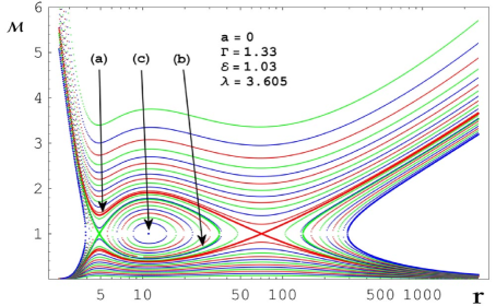
Figure 1: Mach number $v_{\perp}/c_{s}$ versus $r$ (in units of the Schwarzschild radius) for various $\dot{N}/h$. The entropy measure $\cal K$ corresponding to the flows marked by (a), (b) and (c) equals 0.0181289, 0.0188906. 0.0213815, respectively.

To find solutions with at least one regular sonic point, we take the derivative of (3.9) and (3.10) with respect to $r$, which yields

$$n^{\prime}\frac{\dot{N}}{n}+n\left(\frac{\dot{N}}{n}\right)^{\prime}=0,$$ (4.1)

$$w^{\prime}u_{0}+w(u_{0})^{\prime}=0.$$ (4.2)

Substituting $\dot{N}/n$ and $u_{0}$ from (3.9) and (3.10) and using (2.61), equations (4.1) and (4.2) may be written as a system of linear algebraic equations for $w^{\prime}/w$ and $v_{\perp}^{\prime}/v_{\perp}$

$$\frac{w^{\prime}}{w}+c_{s}^{2}\gamma_{\perp}^{2}\frac{v_{\perp}^{\prime}}{v_{\perp}}=-c_{s}^{2}\frac{1}{2}\frac{\Delta^{\prime}}{\Delta}\,,$$ (4.3)

$$\frac{w^{\prime}}{w}+v_{\perp}^{2}\gamma_{\perp}^{2}\frac{v_{\perp}^{\prime}}{v_{\perp}}=-\frac{1}{2}\frac{\Delta^{\prime}}{\Delta}+\frac{1}{2}\frac{B^{\prime}}{B}\,.$$ (4.4)

Obviously, the determinant of the system vanishes at the acoustic horizon owing to (2.19). The system will have a regular solution at the horizon if and only if the right-hand sides of the two equations become equal at the horizon. In this case, the algebraic system (4.3)-(4.4) degenerates at the horizon into one equation. Hence, the condition

$$(1-c_{s}^{2})\frac{\Delta^{\prime}}{\Delta}-\frac{B^{\prime}}{B}=0$$ (4.5)

must hold at the horizon. If this condition is not satisfied, any solution to (4.3)-(4.4) will have no acoustic horizon at all or will have irregular acoustic horizons, i.e., such that the derivatives $v_{\perp}^{\prime}$ and $c_{s}^{\prime}$ approach infinity as one approaches the horizon.

The regularity condition (4.5) gives $c_{s}$ at the horizon in terms of $r_{\rm h}$ but the actual value of $r_{\rm h}$ is yet unknown. To find $r_{\rm h}$, we need to specify the equation of state. Given the equation of state, we can express $w$ in terms of $c_{s}$, substitute $c_{s}$ from (4.5) into (3.10) and thus obtain an equation for $r$. For example, equation (2.62), which follows from the polytropic equation of state (2.56), yields

$${\cal E}\left(\Gamma-2+\frac{\Delta\,B^{\prime}}{B\Delta^{\prime}}\right)=(\Gamma-1)\left(\frac{\Delta^{\prime}}{B^{\prime}}\right)^{1/2}.$$ (4.6)

A solution to this equation for fixed $\lambda$ and $\cal E$ determines the horizon radius $r_{\rm h}$. Equation (4.6) may, in general, have more than one solution. However, not all real solutions are physically acceptable. The positivity of $u_{0}^{2}$ in (3.3) requires

$$g_{\phi\phi}+2\lambda g_{0\phi}+\lambda^{2}g_{00}\leq 0.$$ (4.7)

For a given $\lambda$, this inequality fixes the range of acceptable $r$.

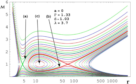
Figure 2: Same as figure 1 for a different flow topology. The entropy measure $\cal K$ corresponding to (a), (b) and (c) equals 0.0158061, 0.0180944 and 0.0206812, respectively.

Once we have $r_{\rm h}$ and $c_{s}$ at the horizon, the constant $\dot{N}/h$ may also be fixed from equation (3.9) evaluated at the horizon. Equations (3.9) and (3.10) then determine the radial dependence of $c_{s}$ and $v_{\perp}$. It is important to emphasize that this procedure determines only a subset of solutions to equations (3.9) and (3.10) (or equivalently (4.3) and (4.4)) which possess sonic points that satisfy the condition (4.5). Any other solution will have singular sonic points or no sonic point at all. This may be seen in figures 1 and 2 where two typical sets of solutions with different topology depending critically on $\lambda$ are plotted for a fixed $\cal{E}$. Solutions are expressed in terms of the so-called Mach number defined as the ratio ${\cal M}\equiv v_{\perp}/c_{s}$. The curves crossing the ${\cal M}=1$ line are transonic and the crossing points are the location of the acoustic horizon. The plots also include the configurations that do not satisfy (4.5) at the acoustic horizon. The plots describe both wind and accretion, depending on the sign of $\dot{N}$ or equivalently of $v_{\perp}$. Each line on the plot represents wind if $\dot{N}<0$ ($v_{\perp}>0$) or accretion if $\dot{N}>0$ ($v_{\perp}<0$). The flow described by line (a) has an X-type sonic point. The flow marked by (b) has two branches, each passing an X-type and ending at a singular sonic point. An isolated O-type sonic point is marked by (c).

Obviously, a smooth flow will have at most one regular sonic point.. Hence, a smooth multitransonic flow is not possible. However, a multitransonic flow with two sonic points and a shock in between may be realized if discontinuous transitions between different lines are allowed.

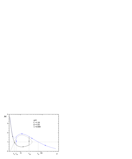
Figure 3: Transonic accretion with two sonic points at $r_{\rm h1}$ and $r_{\rm h2}$ and a shock in between at $r_{\rm sh2}$ (solid line). The dashed line represents an alternative flow with a (unstable) shock at $r_{\rm sh1}$. The parameters are as in figure 1.

The lines in the plots in figures 1 and 2 in general correspond to different constants $\dot{N}/h$ and if the entropy is conserved, there is no way to jump from one line to another. However, instead of keeping the constant ${\cal K}$ fixed, we fix $\dot{N}/h$ and allow ${\cal K}$ to vary from line to line. In this way the jumps between the lines labelled by different ${\cal K}$ will be allowed at those points where the Rankine-Hugoniot conditions are satisfied.

The flows with singular sonic points, i.e., the points where $v_{\perp}^{\prime}$ and $c_{s}^{\prime}$ diverge, will formally have acoustic horizons with infinite surface gravity. This property is generic for inviscid flows [31] and the problem will not appear in a realistic fluid with viscosity. In our case, owing to the shock formation, the flow will actually never reach these points. We assume that a stationary accretion flow goes from infinity where it is subsonic to the first unstable orbit of the black hole. In the example depicted in figure 1 the flow represented by line (a) passes through a regular sonic point. If the Rankine-Hugoniot conditions are met, a jump from a supersonic to a subsonic regime will take place, provided the entropy of the subsonic flow is larger. Since ${\cal K}_{\rm(a)}<{\cal K}_{\rm(b)}<{\cal K}_{\rm(c)}$, the entropy per particle $\sigma$, which increases with ${\cal K}$ according to (2.60), increases going from line (a) towards the point denoted by (c) and hence, a jump from (a) to (b) or to any of the closed loops inside loop (b) is possible. However, the only transition that will eventually result in a stable stationary flow will be a jump from (a) to the subsonic branch of (b). A flow with a similar transition from (a) to one of the closed loops will inevitably end up at a singular sonic point, and hence cannot remain stationary.

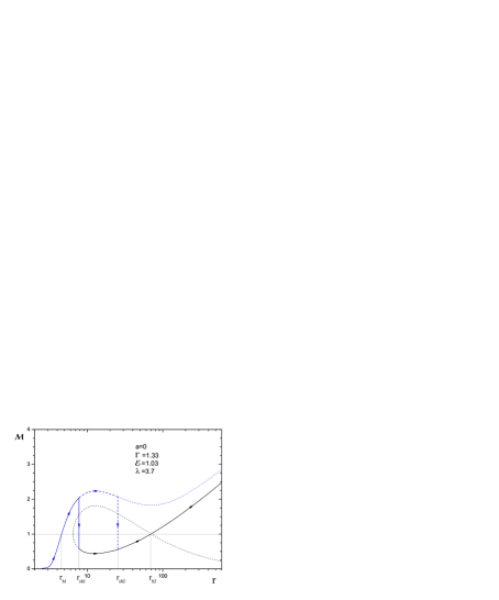
Figure 4: Transonic wind with two sonic points at $r_{\rm h1}$ and $r_{\rm h2}$ and a shock in between at $r_{\rm sh1}$ (solid line). The dashed line represents an alternative flow with a shock at $r_{\rm sh2}$. The parameters are as in figure 2.

The exact location of the shock $r_{\rm sh}$ for a particular flow configuration may be calculated using the Rankine-Hugoniot conditions (2.51)-(2.53) assuming that the outer flow is described by (a) and the inner flow by the subsonic branch of (b). The first two conditions (2.51) and (2.52) are trivially satisfied owing to equations (3.9) and (3.10). The particle number conservation (3.9) across the shock may be written as

$${\cal K}_{1}^{-\frac{1}{\Gamma-1}}\dot{\cal N}_{1}={\cal K}_{2}^{-\frac{1}{\Gamma-1}}\dot{\cal N}_{2}\,,$$ (4.8)

where the subscripts 1 and 2 denote, respectively, the inner and outer boundary values at the shock and

$$\dot{\cal N}\equiv\eta\left(\frac{\Gamma-1}{c_{s}^{2}}-1\right)^{-\frac{1}{\Gamma-1}}v_{\perp}\gamma_{\perp}$$ (4.9)

is a kinematic quantity the change of which across the shock depends on the change of $v_{\perp}$ and $c_{s}$ only. Hence, to make the particle number conserved, a discontinuity of $\dot{\cal N}$ is compensated by a corresponding discontinuity of ${\cal K}$ such that equation (4.8) holds. As a consequence, the entropy per particle $\sigma$ being a continuous function of ${\cal K}$ is not conserved across the shock. The third Rankine-Hugoniot condition (2.53) may now be written as

$$\eta^{\Gamma+1}\left(\frac{\Gamma-1}{c_{s1}^{2}}-1\right)^{-\frac{1}{\Gamma-1}}+(\Gamma-1)c_{s1}^{2}\left(\frac{\Gamma-1}{c_{s1}^{2}}-1\right)^{-\frac{\Gamma}{\Gamma-1}}\dot{\cal N}_{1}^{2}=$$

$$\left[\eta^{\Gamma+1}\left(\frac{\Gamma-1}{c_{s1}^{2}}-1\right)^{-\frac{1}{\Gamma-1}}+(\Gamma-1)c_{s2}^{2}\left(\frac{\Gamma-1}{c_{s2}^{2}}-1\right)^{-\frac{\Gamma}{\Gamma-1}}\dot{\cal N}_{2}^{2}\right]\left(\frac{{\cal K}_{1}}{{\cal K}_{2}}\right)^{\frac{1}{\Gamma-1}},$$ (4.10)

and may be solved for $r$. In figures 3 and 4 we show the solutions for the accretion and wind, respectively, corresponding to the flows depicted in figures 1 and 2. The two possible locations of the shock are shown by vertical lines at $r_{\rm sh1}$ and $r_{\rm sh2}$ with arrows indicating the flow orientation. According to a standard local stability analysis [32], one can show for a multitransonic accretion that only the shock formed in between the middle (indicated by (c) in figures 1 and 2) and the outer sonic point is stable. Hence, in our accretion example in figure 3, the shock at $r_{\rm sh2}$ is stable and the one at $r_{\rm sh1}$ is unstable.

5 Acoustic metric and causal structure

The geometric aspects of the axially symmetric accretion are conveniently described in terms of the acoustic metric defined by (2.17) and the metric discriminant ${\cal D}$ defined by (2.20). In figure 5 we plot the components of the metric tensor as functions of $r$ calculated using equation (2.17) for the transonic accretion flow represented by the solid line in figure 3 and similarly in 6 for the transonic wind of figure 4. For the same flow configurations depicted in figures 3 and 4 we also plot ${\cal D}$ as a function of $r$ in figures 7 and 8, respectively. Clearly, ${\cal D}$ is positive (negative) in the subsonic (supersonic) region. Acoustic horizons are located at the points where the discriminant changes its sign. Depending on the slope of ${\cal D}$ at these points passing in the direction of the flow, we call them acoustic black hole (if the slope is descending) or white hole (if the slope is ascending) horizons. Indeed, for both the multitransonic accretion (figure 3) and the wind (figure 4), the flow at the inner and the outer sonic points denoted by $r_{\rm h1}$ and $r_{\rm h2}$, respectively, goes from subsonic to supersonic; so, according to the classification of Barceló et al [33], there we have acoustic black hole horizons. At the discontinuity $r_{\rm sh1}$ or $r_{\rm sh2}$ the flow goes from supersonic to subsonic and hence observers in the subsonic region of the accretion (between $r_{\rm h1}$ and $r_{\rm sh2}$ in figures 3 and 7 ), and of the wind (between $r_{\rm sh1}$ and $r_{\rm h2}$ in figures 4 and 8) experience a white hole.

Figure 5: The components of the acoustic metric for the accretion flow as in figure 3

Figure 6: The components of the acoustic metric for the accretion flow as in figure 4

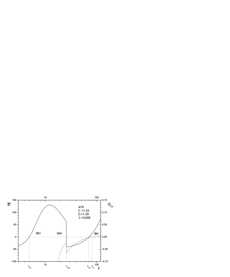
Figure 7: Acoustic metric functions $\cal D$ (solid line) and $G_{00}$ (dashed line) versus $r$ for the multitransonic accretion as in figure 3 with a shock at $r_{\rm sh2}$. Acoustic horizons and their type (from the point of view of an observer in the subsonic region) are indicated by BH (black hole) and WH (white hole).

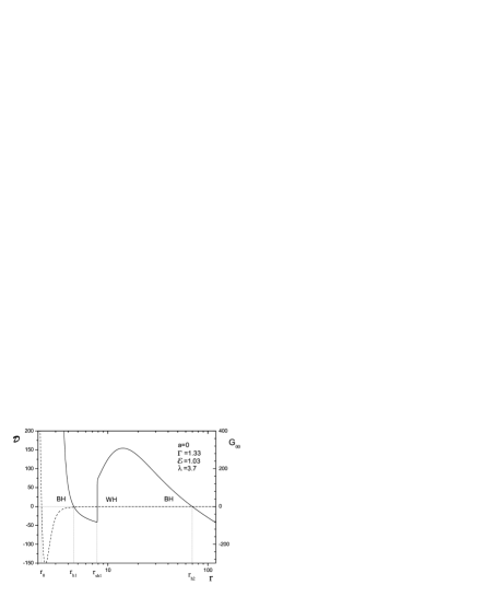
Figure 8: Acoustic metric functions $\cal D$ (solid line) and $G_{00}$ (dashed line) versus $r$ for the multitransonic wind as in figure 4 with a shock at $r_{\rm sh1}$.

In figures 7 and 8 we also plot the metric component $G_{00}$ as a function of $r$ (represented by the dashed line). The point $r_{0}$ where $G_{00}$ changes its sign is the radius of the stationary limit surface and the boundary of the acoustic ergo region.

Figure 9: Acoustic causal structure of the transonic accretion of figure 3 with the null curves $u={\rm const}$ (solid lines) and $w={\rm const}$ (dashed lines).

Figure 10: Acoustic causal structure of the transonic wind of figure 4 with the null curves $w={\rm const}$ (solid lines) and $u={\rm const}$ (dashed lines).

In order to study the causal structure of the axially symmetric acoustic geometry, let us introduce retarded and advanced radial null coordinates $u$ and $w$, respectively. We first make a transformation to the acoustic corotating frame by eliminating the term $G_{0\phi}dtd\phi$ from the acoustic metric. This is achieved by transforming $\phi$ to $\phi^{\prime}$ as

$$d\phi^{\prime}=d\phi+\frac{G_{0\phi}}{G_{\phi\phi}}dt\,,$$ (5.1)

with the remaining coordinates unchanged. This yields the acoustic metric

$$ds^{2}=G_{\mu\nu}^{\prime}dx^{\mu}dx^{\nu},$$ (5.2)

where

$$G_{00}^{\prime}=-\frac{\cal D}{G_{\phi\phi}};\;\;\;\;\;\;G_{0\phi}^{\prime}=0,$$ (5.3)

$$G_{0r}^{\prime}=G_{r0}^{\prime}=G_{0r}-G_{r\phi}\frac{G_{0\phi}}{G_{\phi\phi}},$$ (5.4)

with all remaining components of the acoustic metric unchanged. We then make the transformation

$$du=dt+\frac{1}{c_{+}}dr\,,$$ (5.5)

$$dw=dt+\frac{1}{c_{-}}dr\,,$$ (5.6)

where

$$c_{\pm}=\frac{G_{0r}^{\prime}\pm\sqrt{G_{0r}^{\prime 2}-G_{00}^{\prime}G_{rr}}}{G_{rr}}\,.$$ (5.7)

The acoustic metric at constant $\phi^{\prime}$ is then given by

$$\left.ds^{2}\right|_{\phi^{\prime}={\rm const}}=-\frac{\cal D}{G_{\phi\phi}}dudw\,.$$ (5.8)

The functions $t=t(r)$ at constant $u$ or constant $w$, obtained by integrating

$$t=-\int\frac{1}{c_{\pm}}dr\,,$$ (5.9)

represent, respectively, the right-moving and left-moving sound rays or null-rays [33].

In figures 9 and 10 we plot the $u={\rm const}$ and $w={\rm const}$ lines for the accretion of figure 3 and the wind of figure 4. The divergence of lines at the acoustic horizons towards $t=-\infty$ demonstrate an acoustic black hole. Since the transition from a supersonic to a subsonic region is discontinuous at the shock, the lines have a cusp pointing in the direction of positive $t$. If the transition at the shock were smooth, the null lines would diverge towards $t=+\infty$ as in the white-hole example of Barceló et al [33]. Hence, the cusp indicates a white hole.

6 Surface gravity and Hawking temperature

One of the most interesting aspects of acoustic horizons is the existence of a surface gravity and the associated Hawking radiation. To calculate the analogue surface gravity, we need the derivatives $c_{s}^{\prime}$ and $v_{\perp}^{\prime}$ at the acoustic horizon. Let us consider a regular sonic point, e.g., at $r_{\rm h1}$ or $r_{\rm h2}$ in figures 3-8, first. The case of shock will be discussed afterwards. To calculate $c_{s}^{\prime}$ and $v_{\perp}^{\prime}$ at a regular sonic point, we have to solve two equations. The first one is obtained combining (4.3) and the derivative of (2.62):

$$\frac{4c_{s}^{\prime}}{\Gamma-1-c_{s}^{2}}+\frac{2v_{\perp}^{\prime}}{1-c_{s}^{2}}=-c_{s}\frac{\Delta^{\prime}}{\Delta}\,.$$ (6.1)

The second equation is obtained by eliminating $w^{\prime}/w$ from (4.3) and (4.4) and taking the derivative with respect to $r$ of the equation thus obtained at the horizon. We find

$$4v^{\prime}_{\perp}\gamma^{2}_{\perp}(c^{\prime}_{s}-v^{\prime}_{\perp})+2c_{s}c^{\prime}_{s}\frac{\Delta^{\prime}}{\Delta}=\left(1-c^{2}_{s}\right)\left(\frac{\Delta^{\prime\prime}}{\Delta}-\frac{\Delta^{\prime 2}}{\Delta^{2}}\right)-\frac{B^{\prime\prime}}{B}+\frac{B^{\prime 2}}{B^{2}}\,.$$ (6.2)

Equations (6.1) and (6.2) can now be easily solved for $c_{s}^{\prime}$ and $v_{\perp}^{\prime}$.

The analogue surface gravity $\kappa$ may be calculated with help of the Killing field $\chi^{\mu}$ that is null on the horizon. We start from the expression [8, 10]

$$G^{\mu\nu}n_{\nu}\frac{\partial}{\partial n}(G_{\alpha\beta}\chi^{\alpha}\chi^{\beta})=2\kappa\chi^{\mu},$$ (6.3)

where $\partial/\partial n\equiv n^{\mu}\partial_{\mu}$ denotes the normal derivative at the horizon. Since the definition of surface gravity by equation (6.3) is conformally invariant [34], in the calculations that follow we drop the conformal factor $n/(wc_{s})$ in $G_{\mu\nu}$.

Figure 11: Analogue Hawking temperature at the inner (left) and outer (right) acoustic horizon versus the specific angular momentum of the black hole.

Consider the vector field $L^{\mu}$ defined by (2.8). Its magnitude in the acoustic metric is given by

$$\parallel\!L\!\parallel^{2}\equiv G_{\mu\nu}L^{\mu}L^{\nu}=[1-(1-c_{s}^{2})\gamma_{\perp}^{2}]=\gamma_{\perp}^{2}(c_{s}^{2}-v_{\perp}^{2}).$$ (6.4)

Hence, the vector $L^{\mu}$ is null on the horizon. We now construct a Killing vector $\chi^{\mu}$ in the form

$$\chi^{\mu}=\xi^{\mu}+\Omega_{\rm h}\phi^{\mu},$$ (6.5)

where the Killing vectors $\xi^{\mu}$ and $\phi^{\mu}$ are the generators of the temporal and axial isometry group, respectively. It may be easily verified that if the constant $\Omega_{\rm h}$ coincides with the angular velocity (2.16) evaluated at the acoustic horizon, then $\chi^{\mu}$ becomes parallel to $L^{\mu}$ and hence null on the horizon. Using $\chi^{\mu}=\sqrt{\chi^{\nu}\chi_{\nu}}L^{\mu}$ and the definition (2.8) we find

$$G^{\mu\nu}n_{\nu}=n^{\mu}-\frac{1}{v_{\perp}\gamma_{\perp}}u^{\mu}=-\frac{1}{v_{\perp}}\frac{\chi^{\mu}}{\sqrt{\chi^{\nu}\chi_{\nu}}}$$ (6.6)

at the horizon. Equation (6.3), together with (6.4) and (6.6) yields

$$\kappa=\frac{1}{1-c_{s}^{2}}\sqrt{\frac{\chi^{\nu}\chi_{\nu}}{-g_{rr}}}(v_{\perp}^{\prime}-c_{s}^{\prime}),$$ (6.7)

where it is understood that the derivatives and the quantity $\chi^{\mu}\chi_{\mu}$ are to be taken at the horizon. The corresponding Hawking temperature $T_{\rm AH}=|\kappa|/(2\pi)$ represents the temperature as measured by an observer near infinity. For $\lambda=a=0$, equation (6.7) reduces to (2.42) derived in a different way for a nonrotating fluid in a static background metric.

The norm of the Killing vector $\chi_{\mu}$ is easily calculated from (6.5) using (3.2). We find

$$\sqrt{\chi^{\mu}\chi_{\mu}}=\frac{r\sqrt{\Delta\,B}}{r^{3}+a^{2}r+2Ma^{2}-2\lambda Ma}.$$ (6.8)

We plot the ratio of the analogue Hawking temperature $T_{\rm AH}$ to the black hole Hawking temperature $T_{\rm H}$ at the inner and outer horizons as a function of the black-hole specific angular momentum $a$ (figure 11) and of the disk specific angular momentum $\lambda$ (figure 12). The solid and dashed lines represent the two topologies of figures 1 and 2, respectively. However, whereas the inner and the outer acoustic horizons for the topology of figure 1 belong to the same multitransonic flow connected by a shock (the typical configuration depicted in figure 3), the horizons for the topology of figure 2 belong to disconnected transonic flows marked by (a) and (b) in figure 2. Amazingly, the analogue surface gravity is smooth at the topological transition point.

Note that the analogue Hawking temperature $T_{\rm AH}$ of the outer horizon is much lower than the temperature $T_{\rm AH}$ of the inner horizon, which in turn is, although close in magnitude, typically lower than the black hole Hawking temperature $T_{\rm H}$. This is due to the relatively low specific energy ${\cal E}=1.01$, barely exceeding the rest mass. For a range of larger values of $\cal E$ , e.g., close to 2, the temperature $T_{\rm AH}$ would exceed $T_{\rm H}$ as in the spherically symmetric accretion [3, 6]. However, we have found that in this range of large specific energies a multitransonic behaviour is absent.

Figure 12: Analogue Hawking temperature at the inner (left) and outer (right) acoustic horizon versus the specific angular momentum of the disk for the two topologies depicted in figure 1 (solid line) and figure 2 (dashed line).

Calculation of the surface gravity at the shock is not possible in the present model with no viscosity. The shock may be viewed as a boundary separating two phases of the fluid. The equation of state, and hence the sound speed, as well as the radial component of the fluid velocity, in each phase are different and exhibit discontinuity at the boundary. As a consequence, the surface gravity and the associated Hawking temperature at the shock will be formally infinite. However, in a more realistic situation, the phase boundary, owing to viscosity, will have a finite thickness and discontinuities will be smoothed out. The gradients of $v_{\perp}$ and $c_{s}$ will actually be finite but possibly very large. A similar situation occurs in a non-relativistic acoustic setup in which the boundary of a stable-phase bubble propagates in the surrounding metastable phase [35] and in the ³He-A superfluid where a superluminally moving domain wall soliton provides an analogue event horizon [36, 37].

7 Acoustic superradiance

The existence of an ergo region in the transonic accretion flow as described in sections 4 and 5 suggests the possibility of acoustic superradiance. Acoustic waves entering the ergo region and reflecting from the outer acoustic horizon may experience a coefficient of reflection greater than 1. This effect is a close analogue of superradiant scattering [38, 39] which allows energy extraction from Kerr black holes. Acoustic superradiance has recently been extensively discussed in the context of the draining bathtub [40, 41] and its application to the Bose-Einstein condensate [42].

The quantitative investigation of acoustic superradiance in the accretion disc geometry may be performed in the usual way: First, the variables in (2.24) may be separated using a cylindrical wave ansatz

$$\varphi(t,r,\phi)=\Phi(r)e^{-i\omega t}e^{im\phi}\,,$$ (7.1)

where $\omega$ is real and positive and $m$ a positive integer. Equation (2.24) then reduces to an ordinary second-order differential equation for $\Phi(r)$ which may be solved numerically for suitable boundary conditions. However, this calculation may be quite involved for the transonic flow described in sections 4 and 5 and would go beyond the scope of this paper. Instead, we would like to demonstrate here that the acoustic superradiance occurs in a relativistic transonic axisymmetric flow if

$$0<\omega<m\Omega_{\rm h}\,,$$ (7.2)

where $\Omega_{\rm h}$ is the flow angular velocity (2.16) evaluated at the acoustic horizon. To show this, we follow the procedure outlined in [10].

Using the stress tensor (2.27) and the stationary Killing vector $\xi^{\mu}$ we first construct the analogue “energy current”

$$J_{\mu}=T_{\mu\nu}\xi^{\nu};\;\;\;\;\;J^{\mu}=G^{\mu\nu}J_{\nu}\,,$$ (7.3)

which is conserved, i.e. which satisfies $\nabla_{\mu}J^{\mu}=0$, $\nabla_{\mu}$ being the covariant derivative associated with $G_{\mu\nu}$. Hence if we integrate $\nabla_{\mu}J^{\mu}$ over the region $S$ with the boundary $\partial S$, we find by Gauss’s law

$$\int_{\partial S}dS_{\mu}J^{\mu}=\int_{C}dS_{\mu}J^{\mu}+\int_{\Sigma_{1}}dS_{\mu}J^{\mu}+\int_{\Sigma_{2}}dS_{\mu}J^{\mu}+\int_{\Delta{\mathcal{H}}}dS_{\mu}J^{\mu}=0,$$ (7.4)

where we have chosen $\partial S$ such that it consists of the cylinder $C$ of large radius $R\rightarrow\infty$ and height $\Delta t$, the disc $\Sigma_{1}$ at the bottom of the cylinder extended from the outer acoustic horizon radius $r_{\rm h}$ to $R$, the time translated disk $\Sigma_{2}$ at the top, and the part $\Delta{\mathcal{H}}$ of the outer acoustic horizon ${\mathcal{H}}$ between $\Sigma_{1}$ and $\Sigma_{2}$. The integrals over $\Sigma_{1}$ and $\Sigma_{2}$ cancel by time symmetry, the integral over $C$ represents the net energy flow out of $S$ to infinity, i.e., the difference between the outgoing and incoming energies $E_{\rm out}-E_{\rm in}$ during the time $\Delta t$, whereas the integral over $\Delta{\mathcal{H}}$ represents the net energy flow into the acoustic black hole. Thus we have

$$E_{\rm out}-E_{\rm in}=-\int_{\Delta{\mathcal{H}}}dS_{\mu}J^{\mu}=\int dAdt\,\chi^{\mu}J_{\mu}\,,$$ (7.5)

where we have used $n_{\mu}=-G_{\mu\nu}\chi^{\nu}$ as the outward directed normal to the horizon and $\chi^{\mu}$ is given by (6.5). The integral in (7.5) is taken over the proper volume element $dAdt$ on the acoustic horizon. Using $G_{\mu\nu}\chi^{\mu}\xi^{\nu}=0$ which follows directly from (6.6), a straightforward algebra yields

$$\chi^{\mu}J_{\mu}=\chi^{\mu}\partial_{\mu}\varphi\,\xi^{\nu}\partial_{\nu}\varphi=(\partial_{t}\varphi+\Omega_{\rm h}\partial_{\phi}\varphi)\partial_{t}\varphi.$$ (7.6)

Applying this to (7.1) it follows from (7.5) that the time averaged energy flux across the horizon is given by

$$\frac{1}{\Delta t}(E_{\rm in}-E_{\rm out})=\frac{1}{2}A\,\Phi^{2}\omega(\omega-m\Omega_{\rm h})\,,$$ (7.7)

where $A$ is the proper “area” of the horizon. Thus, in the frequency range of equation (7.2), the energy loss across the horizon is negative and hence superradiance is obtained.

8 Conclusions

In this paper we have studied the phenomena related to the acoustic geometry of the axially symmetric accretion flow. We have discussed the formation of the shock and acoustic horizons using a general relativistic formalism in a model of the flow based on a perfect polytropic gas. We have found that a multitransonic flow can form with two sonic points and a shock in between. Null curves depicted in figures 9 and 10 clearly demonstrate the presence of the acoustic black hole at regular sonic points and of the white hole at the shock.

Multitransonic accretion happens for a range of values of the specific energy density not much exceeding the rest mass. The analogue Hawking temperature of the inner horizon, calculated for a typical set of physical parameters, is lower but close in magnitude to the black-hole Hawking temperature. However, at the middle horizon that forms at the shock location, the surface gravity is formally infinite owing to discontinuities in the speed of sound and the radial velocity. We expect that in a realistic fluid with viscosity, discontinuity will be removed and replaced by a steep slope resulting in a finite but possibly very high analogue Hawking temperature.

References

- [1] Novello, Visser & Volovik (ed.) 2002, Artificial Black Holes. World Scientific, Singapore.
- [2] C. Barceló, S. Liberati, and M. Visser, “Analogue Gravity”, gr-qc/0505065
- [3] T.K. Das, Class. Quantum Grav. 21 (2004) 5253, gr-qc/0408081.
- [4] T.K. Das, “Transonic Black Hole Accretion as Analogue System”, gr-qc/0411006.
- [5] V. Moncrief, Astrophys. J. 235 (1980) 1038-46
- [6] S. Dasgupta, N. Bilic and T. K. Das, Gen. Rel. Grav. 37 (2005) 1877, astro-ph/0501410.
- [7] L.D. Landau, E.M. Lifshitz, The Classical Theory of Fields, (Pergamon, Oxford, 1994) p. 251
- [8] N. Bilić, Class. Quantum Grav. 16 (1999) 3953
- [9] S. W. Hawking and G. F. R. Ellis, The large scale structure of space-time, (Cambridge University Press, Cambridge, 1973).
- [10] R.M. Wald, General relativity, (University of Chicago, Chicago, 1984).
- [11] W. G. Unruh and R. Schutzhold, Phys. Rev. D 68 (2003) 024008
- [12] N.D. Birrell and P.C.W. Davies, Quantum fields in curved space (Cambridge University Press, Cambridge, 1982).
- [13] W. G. Unruh, Phys. Rev. D 51 (1995) 2827.
- [14] T. Jacobson, Phis. Rev. D44 (1991) 1731; Phys. Rev. D 48 (1993) 728; S. Corley and T. Jacobson, Phys. Rev. D 54 (1996) 1568.
- [15] L.D. Landau, E.M. Lifshitz, Fluid Mechanics, (Pergamon, Oxford, 1993) p. 507.
- [16] A.H. Taub, “Relativistic Fluid Mechanics”, Ann. Rev. Fluid Mech. 10 (1978) 301–332
- [17] L.D. Landau, E.M. Lifshitz, Statistical Physics, (Pergamon, Oxford, 1994) p. 125.
- [18] J.M. Bardeen, W.H. Press, and S.A. Teukolski, Astrophys. J. 178 (1972) 347-369
- [19] I. D. Novikov, K. S. Thorne, in C. DeWitt and B. DeWitt, eds., Black Holes (Gordon and Breach, New York (NT), 1973) p. 343.
- [20] M. A. Arbamowicz, W. H. Zurek, Astrophys. J., 246 (1981) 314.
- [21] J. Fukue, Publications of the astronomical society of Japan, 39, no. 2, (1987) 309-327; S. K. Chakrabarti, Astrophys. J. 347 (1989) 365; A. K. Ray and J. K. Bhattacharjee, astro-ph/0307447; P. Barai, T. K. Das, and P. J. Wiita, Astrophys. J. Lett. 613 (2004) L49.
- [22] T. K. Das, Astrophys. J. 577 (2002) 880.
- [23] T. K. Das, 2004, Mon. Not. R. Astron. Soc 349 (2004) 375.
- [24] J. Lense and H. Thirring, Phys. Z. 19 (1919) 156.
- [25] J.M. Bardeen and J.A. Petterson, Astrophys. J. 195 (1975) L65.
- [26] T.J. Maccarone, MNRAS 336 (2002) 1371; J.F. Lu and B. Zhou, Astrophys. J. 635 (2005) L17.
- [27] J.A. Petterson, Astrophys. J. 214 (1977) 550; S. Kumar, MNRAS 233 (1988) 33; M. Demianski and P.B. Ivanov, Astron. Astrophys. 324 (1997) 829.
- [28] P.A. Scheuer and R. Feiler, MNRAS 282 (1996) 291.
- [29] R.P. Nelson and J.C. Papaloizou, MNRAS 315 (2000) 570.
- [30] P.C. Fragile and P. Anninos, Astrophys. J. 623 (2005) 347.
- [31] S. Liberati, S. Sonego, and M. Visser, Class. Quantum Grav. 17 (2000) 2903.
- [32] R. Yang and M. Kafatos, Astron. Astrophys. 295 (1995) 238.
- [33] C. Barceló, S. Liberati, S. Sonego and M. Visser, New J. Phys. 6 (2004) 186, gr-qc/0408022.
- [34] T. Jacobson and G. Kang, Class. Quantum Grav. 10 (1993) L201–L206.
- [35] T. Vachaspati, gr-qc/0312069.
- [36] T.A. Jacobson, G.E. Volovik, Pisma Zh. Eksp. Teor. Fiz. 68 (1998) 833-838; JETP Lett. 68 (1998) 874-880, gr-qc/9811014.
- [37] T.A. Jacobson, G.E. Volovik, Phys. Rev. D 58 (1998) 064021
- [38] Ya. B. Zel’dovich, JETP Lett. 14 (1971) 180; Sov. Phys. JETP 35 (1972) 1085.
- [39] A. A. Starobinskii, Sov. Phys. JETP 37 (1973) 28-32.
- [40] S. Basak and P. Majumdar, Class. Quant. Grav. 20 (2003) 2929; ibid 20 (2003) 3907.
- [41] E. Berti, V. Cardoso and J. P. S. Lemos, Phys. Rev. D 70 (2004) 124006; S. Lepe and J. Saavedra, Phys. Lett. B 617 (2005) 174; T.R. Slatyer, C.M. Savage, Class. Quantum Grav. 22 (2005) 3833-3839; C. Cherubini et al, Phys. Rev. D 72 (2005) 084016; W. T. Kim, E. J. Son and M. S. Yoon, gr-qc/0504127; K. Choy et al, gr-qc/0505163.
- [42] S. Basak, gr-qc/0501097; F. Federici, C. Cherubini, S. Succi and M. P. Tosi, gr-qc/0503089.