Geodesics, the Equivalence Principle and Singularities
in Higher-dimensional General Relativity and Braneworlds

Edward Anderson^1,2,† and Reza Tavakol^2,‡

¹ Department of Physics, P-412 Avadh Bhatia Physics Laboratory, University of Alberta,

Edmonton, Alberta, Canada T6G 2J1;

Peterhouse ,Cambridge U.K. CB2 1RD;

DAMTP, Centre for Mathemetical Sciences, Wilberforce Road Cambridge U.K. CB3 0WA.

² Astronomy Unit, School of Mathematical Sciences, Queen Mary,

University of London, U.K. E1 4NS

The geodesics of a spacetime seldom coincide with those of an embedded submanifold of codimension one. We investigate this issue for higher-dimensional general relativity-like models, firstly in the simpler case without branes to isolate which features are already present, and then in the more complicated case with branes. The framework in which we consider branes is general enough to include asymmetric braneworlds but not thick branes. We apply our results on geodesics to study both the equivalence principle and cosmological singularities. Among the models we study these considerations favour $Z_{2}$ symmetric braneworlds with a negative bulk cosmological constant.

PACS NUMBERS: 04.50.+h, 98.80.Jk

Electronic mail: ^†ea212@cam.ac.uk, ^‡R.Tavakol@qmul.ac.uk

1 Introduction

Higher dimensional general relativity (GR) theories have recently attracted much attention. The main role of the extra dimension in such theories is to provide extra degrees of freedom on the $3+1$ hypersurface which is taken to represent the apparent world. Although these are not leading candidates for fundamental theories, they have been used to study some aspects of string/M-theory.

Examples of such higher-d GR theories include (noncompactified) $(n+1)$-d GR [2] (where the choice of the 3 + 1 apparent world is arbitrary), Kaluza–Klein theory [3] (where one dimension is compactified leading to a $3+1$ apparent world described by GR, electromagnetism and a scalar), low energy string cosmology [4] (based on generalized compactifications), and some of the simpler braneworlds [5, 6, 7, 8, 9] (in which the apparent world consists of matter and tension restricted to a special brane hypersurface and the actual world is this hypersurface together with a surrounding bulk spacetime).

Given that the observed macroscopic apparent world is $(3+1)$-d, an important question concerning such theories is how closely their corresponding $3+1$ apparent worlds resemble the observed world, and in particular how observations made in their apparent worlds can test and set constraints on the full theories themselves.

The first aim of this article is to clarify the extent to which such theories satisfy geodesic postulates similar to those of 4-d GR, concerning the motion of particles and light rays. While works relating the geodesics of an embedded 3 + 1 apparent world spacetime and those of the embedding 4 + 1 spacetime have recently appeared (see e.g [10, 11]), we generalize these and work out further consequences of this relation, for 5-d GR models in Sec. 2 and for a wide range of 5-d GR braneworld models in Sec. 3. We find a number of conditions under which the 3 + 1 and 4 + 1 geodesics coincide on the apparent world. These include the so-called $Z_{2}$ symmetry as one of the most robust conditions that enforces this important coincidence. This provides an important extra physical motivation for the consideration of $Z_{2}$ symmetric brane models at the level of GR, independently of the usual motivations based on heterotic M-theory [12, 7] and mathematical simplicity [12].

Geodesics are central to the study of singularities. Having studied the geodesics in higher-d GR models, the second aim of this article is to consider singularities (and whether there is any hope of their resolution) in these settings. We shall study this question for higher-d GR (Sec. 4), as well as for a range of higher-d GR braneworld models (Sec. 5). We shall see that such models become especially interesting in the latter case, with both $Z_{2}$ and non-$Z_{2}$ models giving rise to a range of new possibilities. We conclude in Sec. 6.

2 Foundations for GR and higher-d GR theories

In this section we shall study the extent to which higher-d GR theories are built on foundations analogous to those of GR. We recall that the conventional formulation of GR has three main postulates. (i) 3 + 1 spacetime is a pseudo-Riemannian manifold, which is assumed to be the arena in which real physical events and interactions take place, (ii) Einstein field equations hold and (iii) light rays and freely-falling non-rotating, test-mass particles respectively follow the null and timelike geodesics of the spacetime. This allows contact to be made with observations, and is intimately connected with the equivalence principle, according to which freely-falling non-rotating test particles follow timelike geodesics irrespective of their composition (see [14, 15] for a thorough discussion).

We note that assumptions made in developing higher-d theories can be viewed as more elaborate versions of the above. This involves defining the roles given both to the hypothesized actual $n$ + 1 world and to the 3 + 1 apparent world. Concerning the field equations, the usual and simplest practice is to take $n=4$ and employ the 4 + 1 Einstein field equations. While this would provide a simple choice for the 4 + 1 field equations, it would cause the 3 + 1 apparent-world field equations to differ from the 3 + 1 GR Einstein field equations, as a result of projections of higher-d matter and ‘matter’ induced terms from the higher-d geometry [2, 6].

A crucial issue in braneworld/higher-d models concerns the precise nature of the bulk/higher dimensions. This can either be specified by a fundamental theory, in which case it would in general constrain the dynamics of the brane/lower-d apparent world with observational consequences; or it can be left free - as is to some extent true in most braneworld models considered so far - in which case the lower-d physics will remain unrestricted, unable to provide constraints which may be compared with observations. Clearly the former is essential for physically complete models. In the following we shall mainly consider vacuum or Einstein space bulks, which cover a range of scenarios [2, 5, 6].

Finally, one would require the analogues of the geodesic postulates in GR, both in order to make contact with observations, and because these are implicit in the set-up of some higher-d scenarios where some fields are assumed to be 4-d while others are allowed to propagate in 5-d. Geodesics are also crucial in discussing singularities for these higher-d GR models. In this section we consider 4 + 1 GR including the assumption that the 4 + 1 version of the equivalence principle holds, in the sense that freely falling non-rotating test-mass particles follow 4 + 1 geodesics irrespective of their composition. Now since all test masses follow the same paths in (4 + 1)-d, they will also appear to follow the same paths from the perspective of any included 3 + 1 apparent worlds. Thus there will be some kind of ‘equivalence principle’ from the apparent world perspective. However, the apparent world will not in general look like a 3 + 1 GR world because the set of curves privileged by free fall in the apparent world will not in general include the 3 + 1 timelike geodesics privileged in 3 + 1 GR. Likewise the apparent world’s set of curves privileged by light rays will not in general include the null geodesics privileged in 3 + 1 GR. This is made clear by the following comparative study of the geodesic equations in each space, which is more general that previous studies [19, 10], since we allow general rather than merely tangential paths from the apparent-world perspective.

Contrast the geodesic equations of 3 + 1 GR

$$0=\dot{\mbox{x}}^{\mbox{\scriptsize{A}}}\mbox{D}_{\mbox{\scriptsize{A}}}\dot{\mbox{x}}^{\mbox{\scriptsize{B}}}$$ (1)

with the geodesic equations of a 4 + 1 bulk

$$0=\dot{\mbox{\bf x}}^{\mbox{\bf{\scriptsize A}}}\mbox{\bf D}_{\mbox{\bf{\scriptsize A}}}\dot{\mbox{\bf x}}^{\mbox{\bf{\scriptsize B}}}.$$ (2)

Splitting these equations with respect to a candidate 3 + 1 apparent-world hypersurface we have

$$0=\left\{\begin{array}[]{c}\dot{x}^{A}\mbox{\bf D}_{A}\dot{x}^{B}+\dot{x}^{z}\mbox{\bf D}_{z}\dot{x}^{B}\\ \dot{x}^{A}\mbox{\bf D}_{A}\dot{x}^{z}+\dot{x}^{z}\mbox{\bf D}_{z}\dot{x}^{z}\end{array}\right\}\mbox{ },$$ (3)

where z is the bulk coordinate, and where we have used the splitting with respect to a $(n-1)+1$ hypersurface for a $(1,0)$ tensor on an $n$ + 1 space, $\dot{\mbox{\bf{x}}}^{\mbox{\scriptsize{\bf A}}}=\{\dot{x}^{A},\dot{x}^{z}\}$. Using the corresponding splitting for the covariant derivative $\mbox{\bf D}^{A}$ as can be simply deduced from e.g [20] and passing to normal coordinates, the geodesic equation (2) becomes

$$0=\left\{\begin{array}[]{c}\dot{x}^{A}D_{A}\dot{x}^{B}-2\dot{x}^{A}{K_{A}}^{B}\dot{x}^{z}+\dot{x}^{z}\frac{\partial\dot{x}^{B}}{\partial z}\\ \dot{x}^{A}D_{A}\dot{x}^{z}+K_{AB}\dot{x}^{A}\dot{x}^{B}+\dot{x}^{z}\frac{\partial\dot{x}^{z}}{\partial z}\end{array}\right\}\mbox{ }.$$ (4)

One can view these as representing the motion under velocity-dependent force terms, including terms similar to the Lorentz force, with $x^{z}$ playing the role of charge and the extrinsic curvature $K_{AB}$ playing that of the electromagnetic field tensor $F_{AB}$. We note that for motions with $x^{z}\neq 0$ and assuming $K_{AB}\neq 0$, one would obtain different 5-d trajectories for different $x^{z}$, similar to the way particles with different charges travel on different paths in nonzero electromagnetic fields.

For the geodesics to coincide, we shall allow an arbitrary matter flow $\dot{\mbox{\bf{x}}}^{\mbox{\bf{\scriptsize A}}}$ and then ask under what conditions would the candidate 3 + 1 apparent world strictly reproduce GR, by demanding that

$$\dot{\mbox{\bf x}}^{\mbox{\bf{\scriptsize A}}}\mbox{\bf D}_{\mbox{\bf{\scriptsize A}}}\dot{\mbox{\bf x}}^{\mbox{\bf{\scriptsize B}}}=\left\{\begin{array}[]{c}\dot{x}^{A}D_{A}\dot{x}^{B}\\ 0\end{array}\right\}\mbox{ }.$$ (5)

One has coincidence if

$$\dot{x}_{z}=0~{}~{}\mbox{ and }~{}~{}K_{AB}=0\mbox{ },$$ (6)

$$\mbox{\sl{or} if }\mbox{ }\mbox{ }\frac{\partial\dot{\mbox{x}}^{A}}{\partial z}=0~{}~{}\mbox{ }\dot{x}^{z}=\mbox{ constant }~{}~{}\mbox{ and }~{}~{}K_{AB}=0\mbox{ }.$$ (7)

These conditions ensure both that the 3 + 1 equivalence principle holds and that no matter leaves the 3 + 1 apparent world.

The condition $K_{AB}=0$, which is crucial in both cases, is termed the totally geodesic condition for a 3 + 1 hypersurface embedded within a 4 + 1 bulk. The significance of $K_{AB}=0$ has already been noted in the higher-d literature (e.g [11]), for the cases with $\dot{x}^{z}=0$. The advantages of not presupposing this condition are twofold. Firstly it leads to the second case above, that is an example of a 3 + 1 world hypersurface which, while totally geodesic, allows flows in the perpendicular direction at the same rate. Furthermore there is no difference between the on-apparent-world components of the flows and the corresponding components of flows on a nearby ‘parallel’ 3 + 1 world. Secondly this highlights the fact that leaking matter and equivalence principle violation effects are two sides of the same coin in setting up apparent worlds within higher-d GR bulks.

While the assumption of total geodesy would ensure that both astronomical observations and equivalence principle experiments are in accord with accepted physics and that no matter would disappear from the 3 + 1 apparent world, it is important to note that 3 + 1 apparent worlds cannot generically be accommodated as totally-geodesic hypersurfaces within e.g 4 + 1 vacuum manifolds. This is due to the fact that the specification of a general apparent world would require full knowledge of the form of its metric $h_{AB}$ (10 independent pieces of information), as well as the simultaneous assumption of total geodesy (i.e. $K_{AB}=0$, which amounts to 10 more pieces of information). But, as $h_{AB}$ and $K_{AB}$ are restricted by 5 constraint equations, this specification is in general impossible. By the Gauss constraint, only those apparent worlds with Ricci scalar $R=0$ can be treated thus. One might attempt to avoid this difficulty by leaving the bulk matter content unspecified, in which case the constraint equations could be viewed as equations to solve for the bulk matter content that permits such a slice to exist. Generically, however, there is no reason for the ensuing bulk matter content to be physically reasonable, which is similar to the related problem in GR where arbitrary specification of the metric on the left hand side of Einstein field equations does not generally result in a reasonable energy momentum tensor on the right hand side, as was pointed out by Synge [22] long ago. As we shall see total geodesy is both restrictive and supplantable for $Z_{2}$ braneworlds (Sec. 3).

One could try to remedy this problem by considering ‘almost total geodesy’, instead, where the ‘almost’ implies ‘within observational bounds’. We recall that observations of bending of starlight by the the Sun and galaxies (by microlensing), together with the observations of the Shapiro effect conform to geodesic motion. Furthermore, the universality of free fall is known extremely accurately for a broad range of compositions. Even though it is not these observations that are under direct consideration here, clearly a substantial breakdown of the geodesic assumption would compromise the interpretation of the above observations within a GR framework. On the other hand these are not clean tests of geodesic motion. Indeed, the presupposition of the geodesic principle runs so deep in the GR literature that we were unable to find how accurately it is known that light and freely-falling particles follow geodesics. Therefore it is possible that perfect and universal geodesic motion only hold approximately were we to live on an apparent world, rather than a 4-d GR world. In that case the fundamental theory should provide convincing (i.e. not fine-tuned) arguments for why the departures from perfect geodesic motion should be small, while the theoretical framework [15] of experimental relativity should provide accurate bounds on this smallness.

There is also the associated difficulty of what would be the physical status of an apparent world, if it leaked matter, even slowly. It might be argued that this problem would be resolved by identifying the apparent world with the hypersurface which ‘goes with the flow’, rather than as a leaky hypersurface which just happens to possess a theoretically-desirable metric. However, two issues would in general still remain: does the apparent world become distorted or crinkled if $K_{AB}$ is inhomogeneous and could the flow lead to ‘spreading/incoherence’, in the sense that particles of different composition or moving at different 3 + 1 velocities could flow at different rates within the 4 + 1 picture, so that an initial thin sheet could become much thicker at later times. [We shall return to this question in Sec. 3].

Finally there is the question of how to mathematically quantify the notion of almost geodesy. Comparison of curves only makes sense to us if they are on the same manifold and if they share endpoints [[23] contains a method of doing this].

3 Do higher-d GR braneworlds have analogous foundations?

In this section we extend the investigation of Sec. 2 to the case of higher-d GR braneworld models in which the apparent world is confined to an infinitely thin brane which generally has both tension and matter. The models considered here have the important advantage over those in Sec. 2 that they can accommodate a wide range of apparent worlds, thus making contact with a broad range of braneworld models [5, 6, 7, 8, 9].

Consider a general notion of braneworld with thin branes which do not necessarily satisfy the $Z_{2}$ symmetry, i.e which have a distinct bulk spacetime either side of the brane. Braneworld scenarios usually involve a more complicated set of physically privileged curves than in GR. In such models, it is usually postulated that gravitons and bulk-species test matter move on 4 + 1 geodesics, while ordinary test matter follows curves that are confined to a 3 + 1 apparent world. Thus these postulates can amount to a significant practical alteration of the foundations of physics. Thus from a 4 + 1 GR perspective the usual notion of geodesics is applied to the 4 + 1 ones, which is now reserved for the motion of speculative bulk matter, while all brane-confined matter fields (test particles, light rays) are postulated to move on 3 + 1 geodesics. Since as we saw above these are not in general among the 4 + 1 geodesics, one is in effect postulating two separate privileged classes of curves for free fall. This, by definition, amounts to equivalence principle violation and in this sense these models are not generally expected to be higher-d GR theories. But unless there is little or no equivalence principle violation, they would not be viable observationally.

We begin our analysis by looking for conditions which ensure that the geodesics on the brane and bulk coincide. We shall use the notation

$$[A]=A_{+}-A_{-}\mbox{ },$$ (8)

$$(A)=A_{+}+A_{-}\mbox{ },$$ (9)

where +, – denote each side of the brane. For tractability we require a number of objects to be continuous across the brane, namely the apparent world metric:

$$[g_{AB}]=0\mbox{ },\mbox{ }$$ (10)

and some velocities

$$[\dot{x}_{A}]=0\mbox{ },\mbox{ }[\dot{x}_{z}]=0\mbox{ }.$$ (11)

Moreover a discontinuity is permitted in $K_{AB}$ in the limit of a thin sheet of matter being sandwiched between the two bulk portions so that [19]

$$-\frac{1}{2}Y_{AB}=[{K}_{AB}-g_{AB}K]\mbox{ }\mbox{ }\Leftrightarrow\mbox{ }\mbox{ }[K_{AB}]=-\frac{1}{2}\left\{Y_{AB}-\frac{Y}{3}g_{AB}\right\}\mbox{ },$$ (12)

for $K$ is the trace of the apparent world’s extrinsic curvature $K_{AB}$ and $Y_{AB}$ is composed of the thin matter sheet energy-momentum $T_{AB}$ and the brane’s tension $\lambda$:

$$Y_{AB}=T_{AB}-\lambda g_{AB}\mbox{ }.$$ (13)

The Einstein field equations for the composite spacetime is then $\mbox{\bf G}_{\mbox{\bf{\scriptsize AB}}}=\mbox{\bf T}_{\mbox{\bf{\scriptsize AB}}}-\Lambda\mbox{\bf g}_{\mbox{\bf{\scriptsize AB}}}-\delta^{(4)}(z)Y_{\mbox{\bf{\scriptsize AB}}}$, where $\mbox{\bf g}_{\mbox{\bf{\scriptsize AB}}}$, $\mbox{\bf G}_{\mbox{\bf{\scriptsize AB}}}$, $\mbox{\bf T}_{\mbox{\bf{\scriptsize AB}}}$ and $\Lambda$ are the bulk metric, Einstein tensor, energy–momentum and cosmological constant respectively.

As regards geodesics, what is relevant on-brane are the geodesic equations with the average bulk contributions. Thus one generally has, in ‘brane-centric’ normal coordinates,

$$0=\left\{\begin{array}[]{c}\dot{x}^{A}D_{A}\dot{x}^{B}-\dot{x}^{A}{(K_{A}}^{B})\dot{x}^{z}+\dot{x}^{z}\frac{\partial\dot{x}^{B}}{\partial z}\\ \dot{x}^{A}D_{A}\dot{x}^{z}+\frac{1}{2}(K_{AB})\dot{x}^{A}\dot{x}^{B}+\dot{x}^{z}\frac{\partial\dot{x}^{z}}{\partial z}\end{array}\right\}\mbox{ }.$$ (14)

The condition for the 3 + 1 and 4 + 1 geodesics to coincide now becomes

$$0=\dot{\mbox{\bf x}}^{\mbox{\bf{\scriptsize A}}}\mbox{\bf D}_{\mbox{\bf{\scriptsize A}}}\dot{\mbox{\bf x}}^{\mbox{\bf{\scriptsize B}}}=\left\{\begin{array}[]{c}\dot{x}^{A}D_{A}\dot{x}^{B}\\ 0\end{array}\right\}\mbox{ }.$$ (15)

which holds if

$$\dot{x}^{z}=0~{}~{}\mbox{and}~{}~{}(K_{AB})=0\mbox{ },$$ (16)

$$\mbox{ or if }\mbox{ }\mbox{ }\frac{\partial\dot{\mbox{x}}^{\mbox{{\scriptsize A}}}}{\partial z}=0\mbox{ , }~{}~{}\dot{x}^{z}=\mbox{ constant }\mbox{ and }~{}~{}(K_{AB})=0\mbox{ }.$$ (17)

Comparing with the previous section, we note that from (12) total geodesy now requires that the on-brane matter has a pure trace energy–momentum tensor. Furthermore, it is now the averaged totally-geodesic condition $(K_{AB})=0$ (also known as $Z_{2}$ symmetry) which ensures the coincidence of the apparent and bulk geodesic equations (i.e. no equivalence principle violation) as well as ensuring that bulk matter does not fall on or off the apparent world. While this condition does not generally hold for braneworld scenarios, it does hold for a range of thin branes. This makes it a far more general condition than total geodesy, since the brane apparent worlds satisfying this condition remain privileged among the more general possibilities by possessing on-brane 4-d and 5-d geodesic coincidence and a sort of neutral stability to falling off the brane.

We note that the absence of $Z_{2}$ symmetry is not immediately disastrous in terms of matter confinement, as one may be able to arrange the apparent world to be identified with the hypersurface which ‘goes with the flow’. However, we shall show below that this is not generally possible. Also, even in presence of confinement, braneworld models may suffer equivalence principle violation by the arguments above. Finally, as we shall see below, $Z_{2}$ symmetry is not the only way to ensure coincidence between geodesics and hence confinement.

One should also bear in mind that the main motivation for considering such models is string/M-theory, within which matter species propagate differently depending on whether they belong to open or closed string multiplets. This would require two distinct types of confinement. Firstly, one would require an approximate confinement whereby bulk ‘closed string’ species do not make the apparent world look overly 5-d. This is modelled by warping as e.g occurs in anti-deSitter-like bulks. Secondly, there is an independent, total confinement of on-brane ‘open string end’ species. From our arguments, one way of attaining this is to invoke $Z_{2}$ symmetric models. These are neutrally stable to constituent bodies accelerating straight off the thin matter sheet.

Despite these appealing features, there are a number of reasons why these mechanisms may not be satisfactory. First, the delta function branes may come with mathematical problems, much as delta-function particles and cosmic strings do. Second, thick branes [25] may actually be more desirable, in which case there may still be 2 sets of privileged curves within them, without a clear notion of which to identify with lower-d geodesics. Thirdly, it is not clear how string-theoretic the models considered in this article really are.

Testing the theories of this section presents additional difficulties. If light is postulated to be totally confined to the 3 + 1 apparent world and to follow geodesics thereon, there is no difference between light propagation on the apparent-world brane and in conventional GR. Thus light deflection cannot be used as a distinguishing test. For equivalence principle tests, one would need to possess a bulk matter particle in order to compare its free fall with that of a particle made of ordinary matter. Were gravitons and massless scalars alone to follow 4 + 1 geodesics, massive test objects could not be built out of 4 + 1 geodesic-traversing matter so no tests of the equivalence principle could ever be affected. In principle one could compare the paths of photons and gravitons, but this would require observations of gravity waves and a clear knowledge that both were emitted simultaneously.

We proceed as follows. The 4 + 1 bulk Einstein field equations are split up as before with respect to a timelike hypersurface, which is moreover now declared to be an apparent-world brane. Thus there are additional discontinuity terms both in the $Z_{2}$ case, and even more so in the asymmetric case.

We present the five ‘constraints’ by adding and subtracting them for the two sides of the brane. Adding the Codazzi constraints,

$$-(j_{B})=D^{A}(K_{AB})-D_{B}(K)\mbox{ },$$ (18)

and subtracting them,

$$-[j_{B}]=D^{A}[K_{AB}]-D_{B}[K]=D^{A}Y_{AB}\mbox{ }.$$ (19)

Adding the Gauss constraints,

$$R+\frac{1}{4}\left\{(K_{AB})(K^{AB})-(K)^{2}\right\}+2\{\rho-\Lambda\}=-\frac{1}{4}\left\{[K_{AB}][K^{AB}]-[K]^{2}\right\}=-\frac{1}{4}\left\{Y_{AB}Y^{AB}-\frac{Y^{2}}{3}\right\}\mbox{ },$$ (20)

and subtracting them,

$$2[\rho-\Lambda]=(K)[K]-(K_{AB})[K^{AB}]=(K_{AB})Y^{AB}\mbox{ }.$$ (21)

In order to have on-brane energy-momentum conservation, one requires $[j_{B}]=0$ which gives $(j_{B})=2j_{B}$ in (18). This precludes a net flow of energy–momentum on or off the brane hypersurface. Also, as was discussed above, thick branes would be prefereable in view of their smooth mathematical properties. In that case it would be natural to have the other components of $[\mbox{\bf{T}}_{\mbox{\scriptsize{\bf AB}}}]$ to be zero, with $[\rho]=0$ being of particular relevance in the above context. Another common choice that is often made is $j_{A}=0$, since in that case the often-imposed ${Z}_{2}$ symmetry, $(K_{AB})=0$, would allow equations (19) and (21) to be solved automatically (the latter for $[\Lambda]=0$), while at the same time simplifying (20). This choice, however, entails further brane-bulk noninteraction. In the case of $j_{A}\neq 0$, on the other hand, ${Z}_{2}$ symmetry is not possible by (18). In that case one would need to consider more general asymmetric bulk braneworld scenarios [8, 9].

3.1 Stability of thin matter sheets/branes

It turns out that in addition to the matter-type-insensitive condition $(K_{AB})=0$, there are also matter-type-specific conditions which ensure the coincidence of 3 + 1 and 4 + 1 geodesics. Here we briefly consider a number of examples:

Single perfect fluid with tension

We seek the conditions that a single perfect fluid would remain on the brane, without assuming any relations between $K^{+}_{AB}$ and $K^{-}_{AB}$. This can be obtained by recalling that the perceived normal acceleration is the averaged one, $<a_{z}>$, given by

$$\{{\sigma+p}\}<a_{z}>=-\frac{1}{2}\{\lambda+p\}(K)\mbox{ }$$ (22)

where $\sigma$ and $p$ are the density and pressure of matter/energy of the apparent world. Therefore, if $\sigma\neq-p$, we obtain an expression for $<a_{z}>$, that is zero if either the fine-tuned on-brane balance $p=-\lambda$ holds or $(K)=0$. If $\sigma=-p$, then either $p=-\lambda$ or $(K)=0$ are required for consistency and we no longer have an expression for $<a_{z}>$.

A number of sub-cases can then be easily studied, including the case of a thin sheet of dust on a hypersurface. In this case $p=0=\lambda$ and we have $<a_{z}>=0$, which shows that a thin sheet of dust stays on whatever hypersurface it is declared to be on without any assumptions about what relation there might be between $K^{+}_{AB}$ and $K^{-}_{AB}$, as was shown by Israel [19].

Including pressure generalizes this condition to

$$\{{\sigma+p}\}<a_{z}>=-\frac{p(K)}{2}\mbox{ }.$$ (23)

So, if $\sigma\neq-p$, we have an expression for $<a_{z}>$, and it is only zero if $p=0$ (the dust case) or $(K)=0$ (the ‘stationary-average’ condition). Thus even though Israel’s result is dust-specific, a weaker result of non-motion holds for perfect fluids, when the two bulk extrinsic curvatures obey $(K)=0$ which is more general than the ‘$Z_{2}$’ or ‘space-symmetric average’ or ‘totally geodesic average’ condition $(K_{AB})=0$. If $\sigma=-p$ (the inflationary case), then if the universe is nonempty, $(K)=0$ is required for consistency and we no longer have an expression for $<a_{z}>$.

Multiple perfect fluids with tension One can also consider multi-fluid models with tension, where for example one has

$$Y_{AB}=\{\sigma_{1}+p_{1}\}u_{1A}u_{1B}-p_{1}g_{AB}+\{\sigma_{2}+p_{2}\}u_{2A}u_{2B}-p_{2}g_{AB}-\lambda g_{AB}$$ (24)

for a two-component non-interacting fluid. In this case (20) implies that

$$<a_{1z}>\{\sigma_{1}+p_{1}\}+<a_{2z}>\{\sigma_{2}+p_{2}\}=-\frac{p_{1}+p_{2}+\lambda}{2}(K)\mbox{ }.$$ (25)

If neither fluid is inflationary (i.e. $\sigma_{1}\neq-p_{1},\sigma_{2}\neq-p_{2}$), then it is impossible to ensure

$<a_{1z}>=0=<a_{2z}>$ unless

$$(K)=0\mbox{ or the fine-tuned on-brane balance}~{}~{}p_{1}+p_{2}=-\lambda$$ (26)

holds. Furthermore, the condition $<a_{1z}>=<a_{2z}>$ is not generic, so the two components of the fluid will generally experience different normal accelerations and move away from the original brane-candidate hypersurface at different rates.

This example demonstrates that one cannot in general associate an intially thin hypersurface of complicated enough composition with a brane, by having it move with ‘the’ transversal flow, as there may simultaneously exist more than one such flow. In the case that (without loss of generality) fluid 1 is inflationary and fluid 2 is not, (25) gives an expression for $<a_{2z}>$, which is zero if either of the conditions (26) hold, while we do not have an expression for $<a_{1z}>$. If both fluids are inflationary, then either of the conditions (26) must hold for consistency and we do not have expressions for either $<a_{1z}>$ or $<a_{2z}>$.

Thus, summarizing (and in all cases assuming $p>-\sigma$), a brane is non-accelerating if: I) It is $Z_{2}$ symmetric, $(K_{AB})=0$, regardless of its (minimally coupled) matter composition. II) It is a ‘stationary-average’ brane, $(K)=0$, and of single perfect fluid composition. III) It is of unrestricted $(K_{AB})$, of single perfect fluid composition and fine-tuned in a special way.

We also note, following [8], that one can think of $[\rho-\Lambda]$ as an external force capable of moving around the above thin matter sheets. We do not consider the possibility of $[\rho]\neq 0$ on the grounds of over-richness of solutions and naturality given that $[j_{b}]=0$ is required for on-brane energy–momentum conservation. While this assumption changes the precise form of the balances for no on-brane perpendicular accelerations of test particles, it does not change the fine-tuned nature of such balances in that they continue to require equating on-brane matter quantities (such as $p$ and $\lambda$) with the a priori unrelated geometrical object $(K)$ alongside the a priori unrelated difference of bulk cosmological constants $[\Lambda]$.

Stability of branes

Finally, an important question concerns the fate of initial thin brane configurations. The general answer to this question clearly lies beyond the scope of the single thin brane considerations here. Our results concerning multi-fluid cases allow some intuition to be gained in this connection. For example, even though pure (single component) dust without tension would remain fixed on the initial brane, implying some form of stability, this would not be the case for a more general multiple component perfect fluid. A simple example is that of 2 dust fluids with tension, in the absence of external forces, which would usually accelerate differently.

Further important questions in this regard are how thick a brane could our world be within experimental bounds? What are the predictions of thick brane physics? Can they thicken too quickly to agree with observations? We note that the assumption of $Z_{2}$ symmetry does not preclude thickening. Also the neutral stability discussed above may not be enough in general: one should also investigate the stability to perturbations, which may or may not be $Z_{2}$ symmetric, depending upon theoretical preference.

4 Singularities in GR and higher-d GR theories

The physically-privileged status of geodesics makes them of fundamental importance in the study of singularities. Even though there is no universally satisfactory definition of singularities [26, 27], they are often defined in terms of geodesic-incompleteness. On the other hand, the study of singularities has been approached in terms of other notions (some physically motivated and some merely convenient), including the expansion and shear of geodesic congruences, energy conditions and curvature scalars.

We study the cosmologies of standard GR, apparent worlds, and bulk worlds in terms of smooth congruences of past-directed normal timelike geodesics with normalized tangents. In each case there is a normal Raychaudhuri equation determining the evolution of the expansion. For example, for the standard GR we have

$$\dot{\mbox{o}}-\frac{\mbox{o}^{2}}{3}={\varsigma}_{\mbox{{\scriptsize AB}}}\varsigma^{\mbox{{\scriptsize AB}}}+\mbox{R}_{\mbox{{\scriptsize AB}}}\mbox{U}^{\mbox{{\scriptsize A}}}\mbox{U}^{\mbox{{\scriptsize B}}}\geq 0\mbox{ }.$$ (27)

Now for initial expansion $\mbox{o}_{0}>0$ this would, under certain global conditions, usually imply the development of caustics which give rise to conjugate points (i.e the intersection points of re-intersecting geodesics). Singularity theorems are thus obtained. In a cosmological context the simplest of these is [28]

Cosmological Singularity Theorem 1: For globally-hyperbolic 3 + 1 GR spacetimes obeying the strong energy condition and such that $\mbox{o}=C\geq 0$ on some smooth (spacelike) Cauchy surface S, then no past-directed timelike curve from S can have greater length than $\frac{3}{|C|}$.

By the definition of Cauchy surface, all past-directed timelike geodesics are among the timelike curves mentioned and are thus incomplete, so the spacetime is singular.

There are a number of other cosmological singularity theorems (see e.g. [29, 23, 30] both to accommodate weaker assumptions and to eliminate a number of pathological cases. These are all phrased in terms of geodesic-incompleteness. We recall that singularity theorems concern the existence of singularities, saying nothing about their qualitative properties. Carrying out a classification program of singularities according to their properties [27] is extremely difficult, and may never be completed [30].

Below, we confine ourselves to the commonly considered curvature singularities, for which at least one spacetime curvature scalar such as the Ricci scalar R or the contracted product of two Ricci tensors $\mbox{R}_{\mbox{{\scriptsize AB}}}\mbox{R}^{\mbox{{\scriptsize AB}}}$ blows up.

Similar results also hold in higher-d. Our aim, however, is the simultaneous consideration of apparent and bulk worlds, in order to understand whether a surrounding actual bulk world can provide a different account of what appears to be singular behaviour on the apparent world. That some singular spacetimes may be ‘embeddable’ in nonsingular ones follows from simple considerations of hypersurface geometry, which reveal that the behaviour of the higher- and lower-d singularities need not be related. We consider this relation below for the simple 4 + 1 GR models, and for braneworld models in Sec. 5. At the outset of each section, we assume that energy conditions hold for both apparent and bulk worlds, though we will consider this crucial issue toward the end of each Section.

First, as discussed in Sec. 2, the geodesics of a 3 + 1 submanifold are not generally among the geodesics of a 4 + 1 embedding space. Then the question of which curves are to be privileged by freely falling particles translates to which curves’ extendibility is in question in the study of singularities. A subcase of this involves the 3 + 1 incompleteness corresponding to the 3 + 1 apparent-world hypersurface becoming tangent to the characteristics of the bulk equations thus forcing the timelike and null geodesics to exit the 3 + 1 apparent-world hypersurface. Also, the 3 + 1 geodesics might be pieces of 4 + 1 geodesics which are extendible only by replacing a piece of the original foliation with a new one that extends into what was originally regarded as the extra d. If one postulates that both 3 + 1 and 4 + 1 geodesics play a part, it is then not clear what is meant by a singularity: exactly which curves are supposed to be incomplete? In particular, this plays a role in the braneworld case of Sec. 5.

Second, the bulk expansion is

$$\Theta=\mbox{\bf h}^{\mbox{\bf{\scriptsize AB}}}\Theta_{\mbox{\bf{\scriptsize AB}}}=\mbox{\bf h}^{zz}\mbox{\bf D}_{z}\mbox{\bf U}_{z}+\mbox{\bf h}^{AB}\mbox{\bf D}_{A}\mbox{\bf U}_{B}=\Theta_{zz}+h^{AB}\{D_{B}U_{A}+U_{z}K_{AB}\}$$ (28)

using the split provided in [20]. Employing the $zz$ component of the definition of the bulk flow shear $\Sigma_{\mbox{\bf{\scriptsize AB}}}$,

$$\Theta=\Sigma_{zz}+\frac{\Theta}{4}\mbox{\bf h}_{zz}+\theta+U_{z}K\mbox{ },$$ (29)

where $\theta$ is the apparent-world expansion, so the balance between the two expansions is

$$\theta=\frac{3}{4}\Theta-\Sigma_{zz}-U_{z}K\mbox{ }.\mbox{ }$$ (30)

This clearly demonstrates that a blow-up in ${\theta}$ need not imply a blow-up in $\Theta$. Instead it could be the shear component $\Sigma_{zz}$ that blows up (Fig 1). Alternatively it could be $U_{z}$ or the trace $K$ of the extrinsic curvature of the 3 + 0 slice with respect to the 4 + 0 slice that blow up. Thus the 4 + 1 spacetime perspective on focusing of geodesics can be completely different from that of some 3 + 1 apparent-world hypersurface. Thus the condition in cosmological singularity theorem 1, $\theta\geq\frac{3}{C^{(3)}}$, neither implies nor is implied by $\Theta\geq\frac{4}{C^{(4)}}$.

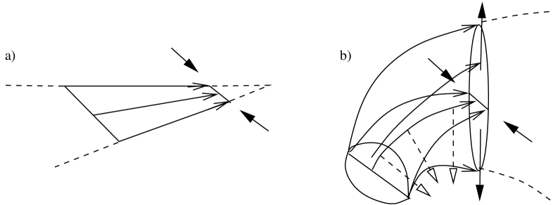
Figure 1: Schematic representation of how lower-d expansion can be higher-d shear or bending. The hollow arrows denote directed geodesics, the black arrows indicate how the congruence is squeezed or deformed and the white arrows are the normals the change in which is extrinsic curvature.

Third, the apparent-world hypersurface components of the higher-d shear are likewise

$$\Sigma_{AB}=\mbox{\bf D}_{A}\mbox{\bf U}_{B}-\frac{\Theta}{4}\mbox{\bf h}_{AB}=D_{A}U_{B}+U_{z}K_{AB}-\frac{\Theta}{4}\mbox{\bf h}_{AB}\mbox{ }.$$ (31)

Using $D_{A}U_{B}=\theta_{AB}=\sigma_{AB}-\frac{\theta}{3}h_{AB}$ together with equation (30) for the apparent-world shear $\sigma_{ab}$, the balance of these components of the two shears is given by

$$\sigma_{AB}=\Sigma_{AB}+\frac{1}{3}\Sigma_{zz}+U_{z}\{Kh_{AB}-K_{AB}\}\mbox{ }.$$ (32)

So a blow-up in $\sigma_{AB}$ could reflect a blow-up in $U_{z}$ or $K_{AB}$ rather that in $\Sigma_{\mbox{\bf{\scriptsize AB}}}$ components.

Fourth, as is already intuitively clear at the level of Gauss’ theorem for embeddings of highly curved 2-d surfaces into flat 3-space, the mathematics of embedding has a means of ‘losing curvature’ in transcending dimension. To consider in particular the balance of the bulk and apparent Ricci scalars, we require the double contraction of the higher-d indefinite signature version of Gauss’ theorem, namely the Gauss constraint

$$2\mbox{\bf R}_{zz}-\mbox{\bf R}=\frac{3}{4}{K}^{2}-L_{\mbox{\bf{\scriptsize AB}}}L^{\mbox{\bf{\scriptsize AB}}}-R\mbox{ }.$$ (33)

The 4 + 1 Einstein field equations also permit the left-hand side of this to be replaced by $2\mbox{\bf T}_{zz}=2\rho$. Thus, clearly, extrinsic curvature can compensate for differences between higher- and lower-d intrinsic curvatures. Our simple point is that one should pay attention to the implications for rigorous embedding mathematics in the cases where lower-d curvature scalars become infinite. It is plausible for some 3 + 1 worlds which have Ricci-scalar curvature singularities $|R|\longrightarrow\infty$, to have corresponding surrounding 4 + 1 worlds in which R (and the 5-d $\mbox{\bf T}_{zz}$) remain finite. For this could be compensated by $|L_{\mbox{\bf{\scriptsize AB}}}L^{\mbox{\bf{\scriptsize AB}}}-\frac{3}{4}{K}^{2}|\longrightarrow\infty$ which could involve

$$|{K}|\longrightarrow\infty\left(\mbox{ i.e.~{} 4 + 0 caustic formation }\right),\mbox{and/or }L_{\mbox{\bf{\scriptsize AB}}}L^{\mbox{\bf{\scriptsize AB}}}\longrightarrow\infty\left(\mbox{ i.e.~{} shear blow up}\right).$$ (34)

If $R\longrightarrow-\infty$, shear blow up will be required.

4.1 Example: the embedding of flat 4-d Robertson–Walker in 5-d Minkowski spacetime

The following simple example illustrates many of the above points and allows further insights to be gained. Consider a 4 + 1 spacetime with the metric (see e.g [32, 33])

$$\mbox{\bf g}_{\mbox{\bf{\scriptsize AB}}}=\mbox{diag}(\mbox{\bf g}_{tt},\mbox{ }h_{ab},\mbox{ }\mbox{\bf g}_{zz})=\mbox{diag}\left\{-z^{2},\mbox{ }t^{\frac{2}{q}}z^{\frac{2}{1-q}}\delta_{ab},\mbox{ }\frac{q^{2}t^{2}}{\{1-q\}^{2}}\right\}\mbox{ },\mbox{ }\mbox{ }q>1.$$ (35)

This is a simple example to treat since: 1) Foliating it with constant $z$ hypersurfaces, a portion of each $z=$ const hypersurface, has induced on it a flat Robertson–Walker metric. In particular, with the coordinates chosen here the $z=1$ hypersurface is the Robertson–Walker metric with scale factor $t^{\frac{1}{q}}$. We note that $q\leq 3$ is required if the dominant energy condition is to hold. For $q\neq 2$ there is a 3 + 1 Ricci scalar curvature singularity. ($q=2$ is the radiation universe whence the energy-momentum trace is zero whence R = 0.)

2) The 4 + 1 spacetime is in fact Minkowski. That such an embedding is possible has long been known [34] and studied elsewhere in the literature [35]. To proceed we first foliate the flat Robertson–Walker metric with constant $t$ surfaces. This gives $\theta=\frac{3}{qt}\longrightarrow\infty$ as $t\longrightarrow 0$, showing that there is 3 + 1 focusing as the Big Bang is approached. Furthermore, only focusing occurs: $\sigma_{AB}=0$. Next one foliates the 4 + 1 spacetime with constant $t$ surfaces. Foliating the 4 + 1 spacetime by constant-$z$ surfaces with Robertson–Walker metrics allows the construction of a congruence by collecting the Robertson–Walker geodesics on each $z=$ const slice. Then the 4 + 1 expansion ${\Theta}=\frac{q+3}{ztq}$ also blows up as $t\longrightarrow\infty$, but there is also a blowup of the corresponding 4 + 1 shear:

$$\Sigma_{\mbox{\bf{\scriptsize AB}}}\equiv\frac{q-1}{4qzt}\mbox{diag}\left\{-h_{ab},\mbox{ }3\mbox{\bf g}_{zz}\right\}\mbox{ }.$$ (36)

Also, whilst both $\theta$ and $\Theta$ still blow up in this case, the former viewed from within the $(z=1)$ 3 + 1 hypersurface corresponds to a genuine 3 + 1 singularity, whilst the latter is a mere caustic in 4 + 1.

Now consider the $(z=1)$ hypersurface as a slice of the 4 + 1 spacetime. The ‘expansion’ and ‘shear’ as regards this slicing are given by

$$K=\frac{q-4}{qt}\mbox{ },\mbox{ }L_{\mbox{\bf{\scriptsize AB}}}=-\frac{1}{4t}\mbox{diag}\left\{3,\mbox{ }t^{\frac{2}{q}}\delta_{ab}\right\}\mbox{ }.$$ (37)

Thus for the physical range of $q$, both $K$ and $L_{\mbox{\bf{\scriptsize AB}}}$ blow up as $t\longrightarrow 0$. So the spacetime includes a $(z=0,t=0)$ point, at which there is a 4 + 0 caustic. These blow-ups combine in $L_{\mbox{\bf{\scriptsize AB}}}L^{\mbox{\bf{\scriptsize AB}}}-\frac{3}{4}{K}^{2}$ to cancel $R$ for all values of $q$; for $q=2$ the ‘shear’ and ‘expansion’ contributions exactly cancel each other. Note that the $q=4$ case is an example of a pure shear blowup. This also provides an example of how theoretically desirable candidate apparent-world hypersurfaces in a bulk can turn out to violate energy conditions on closer inspection.

Although the congruence discussed above is constructed to naturally include the geodesics of all the included Robertson–Walker metrics, these turn out not to be the 4 + 1 geodesics (nor even pieces of them). Changing the coordinates in (35) to standard 4 + 1 Minkowski coordinates, it is easy to show that the Minkowski geodesics pierce the $z=$ constant surfaces which are the Robertson–Walker universes (more significantly in the early universe). As $t\longrightarrow 0$ the $z=$ constant surfaces approach the null cone, thus providing an example of how foliating 3 + 1 hypersurfaces become tangent to the characteristics at the point of interest. The foliation breaks down as $t\longrightarrow 0$ since the family of hypersurfaces of constant $z$ intersect at $t=0$ [see Fig. 2].

Figure 2: Schematic representation of the embedding of flat Robertson–Walker universes into 4 + 1 Minkowski spacetime in the standard 4 + 1 Minkowski coordinates $(T,X_{1},X_{2},X_{3},Z)$. The curved surfaces are the Robertson–Walker spacetimes. As one approaches $T=0$ (corresponding to $t=0$ in Robertson–Walker coordinates), each of these surfaces becomes tangent to the null cone (characteristics of Minkowski). The foliation by these surfaces also becomes bad here because the surfaces intersect. Note also that the Robertson–Walker geodesics move within each of the surfaces whereas the Minkowski geodesics clearly pierce these surfaces. Thus the 3 + 1 and 4 + 1 geodesics in this example are not the same.

To summarize: our studies of examples concerning the relationship between singularities in the 3 + 1 apparent world and 4 + 1 bulk worlds demonstrate that in some cases 3 + 1 singularities may be viewed as projective effects due to a badly-behaved choice of the foliation, e.g one that becomes tangent to the 4 + 1 characteristics. A clear example of this can be seen by (37).

In view of their special nature, however, such examples cannot be taken as representative of generic settings, which are of primary importance in the study of singularities. A first potential source of general theorems are currently-known embedding theorems. Unfortunately, as has been argued elsewhere [37], general statements based on these face difficulties including non-uniqueness, reliance on analytic functions or on high co-dimension. They also have singularity-specific difficulties: (1) the requirement in many embedding theorems for the embedded hypersurface to be entirely of one signature, thus excluding the very points at which the hypersurface goes characteristic. (2) The impossibility of inclusion of the singularity in the set of points on which data is prescribed, since they represent an edge rather than a point of the spacetime. Attempts at their inclusion by providing data ‘right up’ to the edge, cannot always stop the data from becoming badly-behaved, by e.g some components of $K_{{\mbox{{\scriptsize AB}}}}$ becoming infinite when attempting to embed a Ricci scalar singular spacetime into a nonsingular one. (3) The approach to singularities is not always analytic [30].

A second potential source of general theorems are the classical singularity theorems. These readily generalize to higher-d spacetimes, provided that analogous energy conditions are obeyed. However, then even if one were to succeed in excising singularities from a lower-d model, one would typically expect singularities to occur elsewhere in the resultant higher-d models by the higher-d singularity theorems. Also the nature of the corresponding higher-d singularities could be different, specially given that the unrestricted embedding of symmetric spacetimes may result in ‘less symmetric’ higher-d models which by analogy with [39] are capable of exhibiting a wider range of singular (and even nonsingular) behaviours [39]. We add that from the GR perspective it may be viewed as unsatisfactory to replace the unambiguous geodesics with some new privileged curves whose nature depends on the highly nonunique procedure that can be involved in embeddings.

Finally, a key question concerns the nature of bulk matter and the corresponding energy conditions, specially given the absence of observational or theoretical constarints at present. This is important since an assumed bulk strong energy condition need not induce an apparent-world strong energy condition nor vice versa. Minkowski bulks in which anti-deSitter apparent worlds are embedded suffice to illustrate the former, and anti-deSitter bulks in which Minkowski apparent worlds are embedded suffices to illustrate the latter. The crucial point is that the bulk expression $\mbox{\bf R}_{\mbox{\bf{\scriptsize AB}}}\mbox{\bf U}^{\mbox{\bf{\scriptsize A}}}\mbox{\bf U}^{\mbox{\bf{\scriptsize B}}}$ contains not only the apparent-world expression $R_{AB}U^{A}U^{B}$ but also a complicated - albeit easily-computible - combination of terms (involving $\mbox{\bf R}_{Az}$, $\mbox{\bf R}_{zz}$, $K_{AB}$ etc) that arise from the projection of the 4 + 1 Ricci tensor. A related point concerning the strong energy condition is that from the stability condition for geodesics near a totally-geodesic surface [11],

$$\mbox{\bf R}_{\mbox{\scriptsize{\bf AB}}}{\mbox{\bf U}}^{\mbox{\scriptsize{\bf A}}}{\mbox{\bf U}}^{\mbox{\scriptsize{\bf B}}}>R_{AB}U^{A}U^{B}\mbox{ for stability }$$ (38)

and the choice of bulk field equations $\mbox{\bf R}_{\mbox{\scriptsize{\bf AB}}}=0$, one cannot have totally geodesic submanifolds that are simultaneously stable in the above sense and obeying the strong energy condition. Moreover, if there are two distinct notions of privileged curves, the ordinary notion of causality, which physically motivates the dominant energy condition, is undermined.

Note that these complications involving lower- and higher-d energy conditions compromise the apparent-world versions of, among other theorems, the classical cosmological singularity theorems [23]. The points discussed in the last three paragraphs furthermore apply just as well to the case of braneworlds, to which we now turn.

5 Singularities in braneworld models

The fact that 3 + 1 geodesics do not generally coincide with those in 4 + 1 complicates the study and characterization of singularities in these settings. In the case of models satisfying $Z_{2}$ symmetry the geodesics do coincide, thus removing many of these complications. This provides an important motivation for the consideration of $Z_{2}$ symmetric models.

Let the normal congruences of the bulk and apparent world have normalized tangents denoted by

$$\mbox{\bf U}_{\mbox{{\scriptsize\bf A}}}^{\mbox{\scriptsize bulk}}=\mbox{\bf U}_{\mbox{{\scriptsize\bf A}}}^{\mbox{\scriptsize bulk species}}+\mbox{\bf U}_{\mbox{{\scriptsize\bf A}}}^{\mbox{\scriptsize brane species}}\delta^{(4)}(z)\mbox{ }\mbox{ },\mbox{ }\mbox{ }U_{A}^{\mbox{\scriptsize brane}}=U_{A}^{\mbox{\scriptsize bulk species}}+U_{A}^{\mbox{\scriptsize brane species}}\mbox{ }.$$ (39)

The balance of expansions $\theta$ and $\Theta$ can then be arranged to give

$$\frac{3}{4}(\Theta)-(\Sigma_{zz})+U_{z}^{\mbox{\scriptsize bulk species}}(K) = 2\theta\mbox{ },$$ (40)

$$\mbox{ }\frac{3}{4}[\Theta]=[\Sigma_{zz}]+U_{z}^{\mbox{\scriptsize bulk species}}\frac{Y}{6}\mbox{ },$$ (41)

using the fact that $\mbox{\bf U}_{z}^{\mbox{\scriptsize brane species}}$ does not contribute as well as the continuity requirement

$[\mbox{\bf U}_{z}^{\mbox{\scriptsize bulk species}}]=0$. In the $Z_{2}$ case with $\mbox{\bf U}_{z}^{\mbox{\scriptsize bulk-traversing species}}=0$, there is less freedom to compensate for on-brane expansion blow-ups than in the previous section:

$$\frac{3}{4}(\Theta)-(\Sigma_{zz}) = 2\theta\mbox{ },$$ (42)

$$\mbox{ }\frac{3}{4}[\Theta]=[\Sigma_{zz}]\mbox{ }.$$ (43)

Freedom to compensate is also restricted if the brane species have no isotropic contribution $Y=0$ or if the brane is stationary on average, $(K)=0$.

The balance of apparent-world hypersurface components of the shears are given by

$$2\sigma_{AB}=(\Sigma_{AB})+\frac{(\Sigma_{zz})}{3}h_{AB}+U_{z}^{\mbox{\scriptsize bulk species}}\{(K)h_{AB}-(K_{AB})\}$$ (44)

$$0=[\Sigma_{AB}]+\frac{(\Sigma_{zz})}{3}h_{AB}+U_{z}^{\mbox{\scriptsize bulk species}}\frac{Y_{AB}}{2}\mbox{ }.$$ (45)

So $Z_{2}$ symmetry, $\mbox{\bf U}_{z}^{\mbox{\scriptsize bulk species}}=0$, and no brane species matter $Y_{AB}=0$ are conditions which restrict freedom to compensate for on-brane shear blow-ups.

As regards the prospect of Ricci scalar curvature singularity removal, the balance equation in the $Z_{2}$ symmetric case is now given by

$$\frac{1}{4}\left\{\frac{Y^{2}}{3}-Y_{AB}Y^{AB}\right\}-R+2\Lambda=2\mbox{\bf R}_{zz}-\mbox{\bf R}=2\rho\mbox{ }.$$ (46)

Now if $|R|\longrightarrow\infty$ and R and $\rho$ are to remain finite, then we require $\left|\frac{Y^{2}}{3}-Y_{AB}Y^{AB}\right|\longrightarrow\infty$. It is interesting to consider under which circumstances the brane-confined fields’ energy-momentum tensor $Y_{AB}$ remains finite or becomes infinite. It is the former which is unusual as far as standard cosmology is concerned. Although compensation for Ricci scalar blow-up is still possible, while $K_{AB}$ remains finite, through the inverse metric blowing up, $Y_{AB}=-K_{AB}+Kh_{AB}$ will nevertheless diverge if the blow-up is a caustic $|K|\longrightarrow\infty$. Finite density of brane-confined fields is only possible if the blow-up is pure ‘shear’ $|L_{AB}L^{AB}|\longrightarrow\infty$ and due to $h^{AB}$ rather than $L_{AB}$ blowing up.

Also, quite unlike GR, there is a possibility here for two quantities, which are measurable from within the apparent world, to both blow up and yet produce a bulk world which is nonsingular, without resorting to assumptions about any inaccessible bulk parameters. Thus given the novel physical interpretation placed on $[K_{AB}]$ in braneworld models, the Ricci scalar $R$ and brane-confined fields’ energy-momentum $Y_{AB}$ could both blow up, but in such a way that the first and second terms on the left hand side of (46) cancel each other.

In the non-$Z_{2}$ case, there is an extra term $(K_{AB})(K^{AB})-(K)^{2}$ on the left hand side which could be used to balance the Ricci scalar singularity. The brane-confined species’ energy-momentum tensor $Y_{AB}$ is free to remain finite in this case, as it is unrelated to $(K_{AB})$.

5.1 Examples

The above considerations allow a clearer understanding of specific examples of ‘unusual’ singular behaviour considered in the literature. One recent example is given in [31], where in the light of our discussions above it is the curvature blow-ups that are compensated by the extrinsic curvature blow-ups, thus keeping 4 + 1 Ricci curvature finite. We can also answer the question raised in that paper, namely whether braneworlds that are more general than isotropic can have unusual singularities. According to our results here, the answer is in principle yes, in the sense that the required balances are in principle possible for the fully general braneworld field equations in the $Z_{2}$ case and even more so in the non-$Z_{2}$ case. What is not, however, known a priori is whether these possibilities typically occur for the fully general braneworld field equations.

As another example, we further study the example of a bulk anti-deSitter metric given in [10]:

$$\mbox{\bf g}_{\mbox{\bf{\scriptsize AB}}}=\mbox{diag}(\mbox{\bf g}_{tt},\mbox{ }h_{ab},\mbox{ }\mbox{\bf g}_{zz})=\mbox{diag}\left\{-\left\{1+\frac{z^{2}}{l^{2}}\right\},z^{2}S_{ab}^{(3)},\left\{1+\frac{z^{2}}{l^{2}}\right\}^{-1}\right\}$$ (47)

(with coordinates $t$, $\theta$, $\phi$, $\psi$, $z$), where $l$ is some ‘anti-deSitter length’ closely related to the bulk cosmological constant $\Lambda$ and ${S_{ab}}^{(3)}$ is the 3-sphere which we coordinatize by the angles $\theta$, $\phi$, $\psi$. This bulk contains a brane that is a closed Robertson–Walker universe obtained by setting $r=a$ to be the solution of the braneworld version of the Friedmann equation and $t$ to be the solution of $-(1+a^{2}/l^{2})(dt/d\tau)^{2}+(1+a^{2}/l^{2})(da/d\tau)^{2}=-1$.

Using $a=t$ and leading on from a comment in [10], our first point is that this means that the brane becomes tangent to the characteristics of the bulk anti-deSitter spacetime at these singularities. Consequently certain embedding theorems are not applicable there.

Secondly, using the asymptotic solution given in [10], we find that the asymptotic form of the induced 4-metric,

$$h_{AB}=\mbox{diag}\left\{-\left\{1+\frac{t^{2}}{l^{2}}\right\},t^{2}S^{(3)}_{ab}\right\}$$ (48)

(with coordinates $t$, $\theta$, $\phi$, $\psi$), obtained by using $z=a=t$ in (47), has a Ricci curvature singularity $R\sim 1/t^{2}$ as $t\longrightarrow 0$ which corresponds in each case (each with its own choice of $t$) to the approach to the singularity. On the other hand, the anti-deSitter bulk remains perfectly finite there. What happens is that both $L_{\mbox{{\scriptsize AB}}}L^{\mbox{{\scriptsize AB}}}$ and $K^{2}$ blow up as $\sim 1/t^{2}$ so as to compensate for the on-brane Ricci curvature singularity. Moreover, in this example, $K_{AB}$ remains finite, while it is the inverse induced metric that blows up. Nevertheless, the brane-confined matter energy-momentum tensor blows up, because $Y_{AB}=-K_{AB}+Kh_{AB}$ and $K$ blows up. This provides an example of a singularity from the on-brane perspective which is balanced from the bulk perspective such that the blow-up of the brane-confined fields’ energy-momentum cancels out the blow-up of the on-brane Ricci scalar.

Finally, other on-brane Robertson–Walker universes have been considered [31, 40] where derivatives of the scale factor blow-up rather than the scale factor shrinking to zero. These serve as additional examples of behaviours qualitatively different from the Big Bang, but are not connected to the types of balances discussed in this paper.

To summarize, we have shown that there is definitely scope in braneworld models for two distinct notions of physically privileged curves to coexist. Thus the notion of ‘singular’ is even more complicated than in GR case since one would have to consider the extendibility for two congruences of privileged curves of different dimension. Also, as pointed out in [41, 10, 24], assigning roles to both higher-d and lower-d geodesics leads in some cases to amelioration of the apparent world’s horizon problem. We should point out that this too is not solely a feature of braneworlds, but that it is shared by the simpler, not totally-geodesic, models considered in the previous section. We also point out that whenever this amelioration occurs, then the apparent-world dominant energy condition loses physical motivation. Conversely, when some 3 + 1 geodesics permit faster travel than those in 4 + 1, the bulk dominant energy condition loses physical motivation. This is a disturbing legacy given the technical importance of energy conditions, and in particular the dominant energy condition which is currently required, for example, for the positive energy theorem and the zeroth law of black hole mechanics to hold. So such a resolution of the horizon problem would come hand-in-hand with losing understanding of compact object astrophysics.

We also emphasize that the strong energy condition is compromised in braneworlds, both as in Sec. 4.1 as well as for other braneworld reasons. To see this consider the apparent-world Raychaudhuri equation

$$\dot{\theta}=-\frac{\theta^{2}}{3}+\left\{(K)(K_{AB})-(K_{AC})({K^{C}}_{B})+\mbox{Lin}_{AB}+\mbox{Quad}_{AB}\right\}U^{A}U^{B}$$ (49)

where Lin_AB and Quad_AB are linear and quadratic matter terms respectively. Thus even in the $Z_{2}$ case the presence of quadratic matter terms can interfere with establishing an inequality along the lines of the strong energy condition, while in the non $Z_{2}$ case geometrical terms that are untied to matter content can additionally interfere. Thus in GR-based braneworlds, apparent-world versions of the classical singularity theorems (listed in [23]) appear compromised. One problem that can be alleviated in braneworlds is that for bulks with a pure negative cosmological constant, our conclusion in Sec. 4.2, using the stability results from [11] concerning the stability of geodesics on a submanifold to bulk perturbations not being compatible with the strong energy condition on that manifold, does not hold. This is another reason to choose negative cosmological constant bulks.

Moreover, other complications can occur for certain braneworld models with anti-deSitter-like bulks, which though desirable for their confining properties, do not satisfy the weak energy condition. This compromises the bulk versions of one of the classical singularity theorems and of the third law of black hole mechanics. Furthermore, anti-deSitter-like bulks have Cauchy horizons [43] and thus are not globally hyperbolic. This compromises the bulk version of cosmological singularity theorem 1, although the other classical singularity theorems (see [23]) survive this pitfall since they do not require global hyperbolicity. It should also be noted that ‘global hyperbolicity of the apparent world’ may be compromised through bulk influences. This would cause an apparent-world analogue of cosmological singularity theorem 1 to lose its motivation.

6 Conclusion

We have shown that the geodesics of a codimension 1 submanifold are not generically among those of the manifold. One consequence is that the contents of a given submanifold which has been declared as the apparent world may have a propensity to fall off it. Another is that the equivalence principle may no longer hold if 3 + 1 GR is replaced by such a submanifold embedded in a higher-d bulk. For, free fall may acquire an element of composition dependence or may cease to be along the 3 + 1 timelike geodesics of the submanifold. Even though it is true that totally-geodesic submanifolds have geodesics which coincide with those of the surrounding bulk, such worlds are not generic. Also it is not clear that submanifolds that are not branes can serve as apparent worlds. In principle observers may move on a submanifold by appropriate choice of motion. The question, however, is what obliges observersto move on that submanifold? Can matter leave that submanifold even if undergoing forced (rather than geodesic) motion and would an observer whose motion is restricted to that submanifold (by choice or otherwise) notice its disappearance?

In models with branes, however, there is confinement by fiat (some species are declared to be brane-confined fields and observers could be confined by virtue of being made out of these - e.g Standard Model fields) while there is also approximate confinement by warping [whereby bulk-traversing species look very (3 + 1)-d also]. There is evidence that this approximate confinement is within acceptable experimental bounds for at least some braneworld models [5, 44]. For a general thin asymmetric braneworld, bulk and brane geodesics will not in general coincide, so bulk-propagating and brane-confined matter test-bodies undergo distinct free fall: there is in principle equivalence principle violation and on-brane gain or loss of bulk species matter. Moreover, at the level of these GR-like braneworld models, $Z_{2}$-symmetric braneworlds have apparent and bulk geodesic coincidence on the apparent-world brane while being considerably more general that totally-geodesic submanifolds. Thus we argue that these are ‘more like GR’ than asymmetric brane models, which makes them more plausible in themselves within the GR-like braneworld setting, quite apart from $Z_{2}$ symmetry being a feature of at least some phenomenological string-theoretic scenaria [45]. Establishing that was the first aim of this article, alongside constructing a list of aspects of asymmetric braneworlds that are rather more complicated than one might naïvely expect from studying $Z_{2}$ worlds. We also point out that it is not entirely clear whether the idea of brane-confined matter is compatible with GR, in the sense that were the framework of study general enough to include thick branes, could initially-thin branes rapidly become thick?

As regards singularities, we showed that in brane-free models there are already simple balances whereby the bulk and apparent-world versions of the objects used in the study of singularities may greatly differin behaviour. This affects curvature singularities and, more significantly, the energy conditions on which many theorems rest. While these balances permit some curvature singularities to be removed by transcending dimension, this can sometimes be mere alteration or displacement rather than true removal of singularities. We showed that all these phenomena are compounded by including effects due to branes. Again, non-$Z_{2}$ braneworlds open up new possibilities while complicating the definition of a singularity, by complicating the issue of exactly which curves are supposed to be incomplete. On the other hand $Z_{2}$ braneworlds are more reassuringly GR-like. Nevertheless, even these are subject to difficulties due to the bulk and apparent energy conditions not matching up.

Acknowledgements

We would like to thank Malcolm MacCallum, Gary Gibbons and Sanjeev Seahra for fruitful discussions, and Clifford Will and Jurgen Ehlers for comments. RT thanks Miguel Vazquez-Mozo and Kerstin Kunze for helpful discussions. EA thanks PPARC, Peterhouse Cambridge and the Killam Foundation for funding over the years in which this work was done, and Queen Mary London for Visitor status.

References

- [1]
- [2] P.S. Wesson and J. Ponce de Leon, J. Math. Phys. 33 3883 (1992); J.M. Overduin and P.S. Wesson, Phys. Rept. 283 303 (1997), gr-qc/9805018; P.S. Wesson, Space-Time-Matter (World Scientific, Singapore 1999). (We take additional interpretative components therein to be options we do not pursue in this paper).
- [3] See e.g T. Appelquist, A. Chodos and P.G.O. Freund, Modern Kaluza–Klein Theories (Addison–Wesley, Reading MA. 1987); M.J. Duff, Talk delivered at the Oskar Klein Centenary Nobel Symposium, hep-th/9410046.
- [4] See e.g J.E. Lidsey, D. Wands and E.J. Copeland, Phys. Rept. 337 343 (2000), hep-th/9909061.
- [5] L. Randall and R. Sundrum, Phys. Rev. Lett. 83 3370 (1999), hep-ph/9905221; 4690 (1999), hep-th/9906064.
- [6] T. Shiromizu, K-i. Maeda and M. Sasaki, Phys. Rev. D62 024012 (2000), gr-qc/9910076.
- [7] R. Maartens, Living Reviews Relativity 7 7 (2004), gr-qc/0312059.
- [8] R.A. Battye and B. Carter, Phys. Lett. B509 331(2001), hep-th/0101061.
- [9] A-C. Davis, I Vernon, S.C. Davis and W.B. Perkins, Phys. Lett. B504 254 (2001), hep-ph/0008132; R.A. Battye, B. Carter, A. Mennim and J-P. Uzan, Phys. Rev. D64 124007 (2001), hep-th/0105091; L.A. Gergely, Phys. Rev. D68 124011 (2003), gr-qc/0308072; L.A. Gergely, E. Leeper and R. Maartens, Phys. Rev. D70 104025 (2004), gr-qc/0408084; L.A. Gergely and R. Maartens, Phys. Rev. D71 024032 (2005), gr-qc/0411097.
- [10] H. Ishihara, Phys. Rev. Lett. 86 381 (2001), gr-qc/0007070.
- [11] S.S. Seahra, Phys. Rev. D68 104027 (2003), hep-th/0309081.
- [12] P. Brax, C. van de Bruck, A–C. Davis, Rept. Prog. Phys. 67 2183 (2004), hep-th/0404011.
- [13] For a historical account, see P. Havas in Einstein and the History of General Relativity, ed. D. Howard and J. Stachel (Birkhäuser, Boston, 1989). For remaining controversies, see J. Ehlers GRG 11 proceedings, ed. M.A.H. MacCallum (1987); J. Ehlers and R. Geroch, Ann. Phys. N.Y. 309 232 (2004), gr-qc/0309074.
- [14] F.A.E. Pirani, in ‘Lectures on General Relativity’ Brandeis Summer Institute in Theoretical Physics (Prentice-Hall, Inc. New Jersey 1964); I. Ciufolini and J.A. Wheeler, Gravitation and Inertia (Princeton University Press, Princeton 1996).
- [15] C.M. Will, Living Rev. Rel. 4 4 (2001), gr-qc/0103036.
- [16] D. Lovelock, J. Math. Phys. 12 498 (1971).
- [17] D.J. Gross and J.H. Sloan, Nu. Phys. B291 41 (1987).
- [18] J.E. Kim, B. Kyae and H.M. Lee, Nucl. Phys. B582 296 (2000), Errata B591 587 (2000), hep-th/0004005; S. Nojiri and S.D. Odintsov, 2000 JHEP 0007 049, hep-th/0006232; M. Cvetic, S. Nojiri and S.D. Odintsov, 2002 Nucl. Phys. B 628 295, hep-th/0112045; I.P. Neupane, 2001 Phys. Lett. 512 137, hep-th/0104226; I.P. Neupane, 2002 Nucl. Phys. B 621 388, hep-th/0104227; B. Abdesselam and N. Mohammedi, Phys. Rev. D65 084018 (2002), hep-th/0110143; C. Charmousis, J-F. Dufaux, Class. Quantum Grav. 19 4671 (2002), hep-th/0202107. E. Gravanis and S. Willison, Phys. Lett. B562 118 (2003), hep-th/0209076; J.E. Lidsey and N. J. Nunes, Phys. Rev. D67 103510 (2003), astro-ph/0303168; K-i. Maeda and T. Torii, Phys. Rev. D69 024002 (2004), hep-th/03090152; M.H. Dehghani, Phys. Rev. D70 064009 (2004), hep-th/0404118.
- [19] W. Israel, Nuovo Cim. B44 1, (1966), erratum B48 463, (1967).
- [20] K.V. Kuchař, J. Math. Phys. 17 792 (1976).
- [21] It is an obvious consequence of Gauss–Weingarten, specifically made in L.P. Eisenhart, Riemannian Geometry (Princeton University Press, Princeton, 1949).
- [22] J.L. Synge, page 189-190 of Relativity: the general theory (North Holland, Amsterdam 1960).
- [23] R.M. Wald General Relativity (University of Chicago Press, Chicago, 1984).
- [24] D.J.H. Chung, E.W. Kolb and A. Riotto, Phys. Rev. D64 043503 (2001), hep-ph/0008126.
- [25] F. Bonjour, C. Charmousis and R. Gregory, Phys. Rev. D62 083504 (2000), gr-qc/0002063; E. Kiritsis, N. Tetradis and T. Tomaras; JHEP 0108 012 (2001), hep-th/0106050; S. Kobayashi, K. Koyama and J. Soda, Phys. Rev. D65 064014 (2002), hep-th/0107025; P. Mounaix and D. Langlois, Phys. Rev. D65 103523 (2003), gr-qc/0202089; C. Barceló and A. Campos Phys. Lett. B563217 (2003), hep-th/0206217; R. Mansouri, M. Borhani and S. Khakshournia, Int. J. Mod. Phys. A19 4687 (2004) hep-th/0301228; K. Ghoroku and M. Yahiro, hep-th/0305150; D. Bazeia, C. Furtado and A.R. Gomes, JCAP 0402 002 (2004), hep-th/0308034; D. Bazeia and A.R. Gomes, JHEP 0405 012 (2004), hep-th/040314; J. Vinet and J.M. Cline, Phys. Rev. D70 083514 (2004), hep-th/0406141; R. Koley and S. Kar, Mod. Phys. Lett. A20 363 (2005), hep-th/0407159; J. Vinet, Int. J. Mod. Phys. A19 5295 (2004), hep-th/0408082.
- [26] C.W. Misner, Lectures in Applied Mathematics 8 (American Mathematical Society, 1967); R. Geroch, Ann. Phys. (N.Y.) 48 526 (1968).
- [27] G.F.R. Ellis and B.G. Schmidt, Gen. Rel. Grav. 8 915 (1977).
- [28] S.W. Hawking, Proc. Roy. Soc. Lond. A294 511 (1966).
- [29] See e.g S.W. Hawking and G.F.R. Ellis, The large-scale structure of space-time (Cambridge University Press, Cambridge 1973).
- [30] C.J.S. Clarke The Analysis of Space-Time Singularities (Cambridge University Press, Cambridge 1993).
- [31] Y. Shtanov and V. Sahni, Class. Quant. Grav. 19 L101 (2002), gr-qc/0204040.
- [32] J. Ponce de Leon, Gen. Rel. Grav. 20 1115 (1988).
- [33] P.S. Wesson, Mod. Phys. Lett. 7 921 (1992); P.S. Wesson, Astrophys. J. 394 19 (1992); D.J. McManus, J. Math. Phys. 35 4889 (1994); A.A. Coley and D.J. McManus, J. Math. Phys. 36 335 (1995); S.S. Seahra and P.S. Wesson, Class. Quantum Grav. 19 1139 (2002), gr-qc/0202010.
- [34] H.P. Robertson, Rev. Mod. Phys. 5 62 (1933).
- [35] O. Heckmann and E. Schüking, in Gravitation: an Introduction to Current Research ed L. Witten (Wiley, New York 1962); J. Rosen, Rev. Mod. Phys. 37 204 (1965); D. Lynden-Bell, J. Katz and I.H. Redmount, Mon. Not. R. Astr. Soc. 239 201 (1989); W. Rindler, Phys. Lett. A276 52 (2000); M. Lachièze-Rey, Astron. Astrophys. 364 894 (2000), astro-ph/0010163.
- [36] H. Stephani, D. Kramer, M.A.H. MacCallum, C. Hoenselaers and E. Herlt, Exact Solutions to Einstein’s Field Equations Second Edition (Cambridge University Press, Cambridge 2003); G. Abolghasem, A.A. Coley and D.J. McManus, J. Math. Phys. 37 361 (1996).
- [37] E. Anderson, gr-qc/0409122.
- [38] G.W. Gibbons, G.T. Horowitz and P.K. Townsend, Class. Quantum Grav. 12 297 (1995), hep-th/9410073.
- [39] A. Krasiński, Inhomogeneous Cosmological Models (Cambridge University Press, Cambridge 1997).
- [40] N. Deruelle and T. Dolezel, Phys. Rev. D62 103502 (2000), gr-qc/0004021.
- [41] D.J.H. Chung and K. Freese, Phys. Rev. D62 063513 (2000), hep-ph/9910235; R.R. Caldwell and D. Langlois, Phys. Lett. B511 129 (2001), gr-qc/0103070; E. Abdalla, B. Cuadros-Melgar, S-S. Feng and B. Wang, Phys. Rev. D65 083512 (2002), hep-th/0109024; E. Abdalla, A. Casali and B. Cuadros-Melgar, Nu. Phys. B644 201 (2002), hep-th/0205203; E. Abdalla and B. Cuadros-Melgar, Phys. Rev. D67 084012 (2003), hep-th/0209101; B. Cuadros-Melgar, Class. Quant. Grav. 21 2669 (2004), hep-th/0303131
- [42] S. Mukohyama, T. Shiromizu and K-i. Maeda, Phys. Rev. D62 024028 (2000), hep-th/9912287.
- [43] A. Chamblin and G.W. Gibbons, Phys. Rev. Lett. 84 1090 (2000), hep-th/9909130; M. Sasaki, T. Shiromizu and K-i. Maeda, Phys. Rev. D62 024008 (2000), hep-th/9912233.
- [44] J. Garriga and T. Tanaka, Phys. Rev. Lett. 84 2778 (2000), hep-th/9911055.
- [45] P. Hořava and E. Witten Nucl. Phys. B460 506 (1996); B475 94 (1996).