Spacetime symmetries and varying scalars

Abstract

This talk discusses the relation between spacetime-dependent scalars, such as couplings or fields, and the violation of Lorentz symmetry. A specific cosmological supergravity model demonstrates how scalar fields can acquire time-dependent expectation values. Within this cosmological background, excitations of these scalars are governed by a Lorentz-breaking dispersion relation. The model also contains couplings of the scalars to the electrodynamics sector leading to the time dependence of both the fine-structure parameter $\alpha$ and the $\theta$ angle. Through these couplings, the variation of the scalars is also associated with Lorentz- and CPT-violating effects in electromagnetism.

1 Introduction

Despite its phenomenological success, the Standard Model of particle physics leaves unresolved a variety of theoretical issues. Substantial experimental and theoretical efforts are therefore directed toward the search for a more fundamental theory that includes a quantum description of gravity. However, most quantum-gravity effects in virtually all leading candidate models are expected to be minuscule due to Planck-scale suppression.

Recently, minute violations of Lorentz and CPT symmetry have been identified as promising Planck-scale signals.[1] The idea is that these symmetries hold exactly in established physics, are accessible to ultrahigh-precision tests, and can be broken in various quantum-gravity candidates. As examples, we mention strings,[2] spacetime foam,[3, 4] nontrivial spacetime topology,[5] loop quantum gravity,[6] and noncommutative geometry.[7]

The emerging low-energy effects of Lorentz and CPT breaking are described by the Standard-Model Extension (SME).[8] The SME is a field-theory framework at the level of the usual Standard Model and general relativity. Its flat-spacetime limit has provided the basis for numerous experimental and theoretical studies of Lorentz and CPT violation involving mesons,[9, 10, 11, 12] baryons,[13, 14, 15] electrons,[16, 17, 18] photons,[19] muons,[20] and the Higgs sector.[21] We remark that neutrino-oscillation experiments offer the potential for discovery.[8, 22, 23]

Varying scalars are another feature of many approaches to fundamental physics. Effective couplings, for instance, typically acquire time dependencies in models with extra dimensions.[24] Another class of models contains scalar fields, which can acquire time-dependent expectation values driven by the expansion of the universe. For example, in modern approaches to cosmology, such as quintessence,[25] k essence,[26] or inflation,[27] scalar fields are frequently invoked to explain certain observations.

In the present talk, it is demonstrated that the above potential quantum-gravity features are interconnected. In particular, spacetime-dependent scalars are typically associated with Lorentz and possibly CPT violation. In Sec. 2, general arguments in favor of this claim are given. For further illustrations and some specific results, a toy model is introduced in Sec. 3. Lorentz violating effects within the scalar sector of our toy cosmology are discussed in Sec. 4. Section 5 discusses the Lorentz and CPT breaking in the electrodynamics sector of the model. Section 6 contains a brief summary.

2 General arguments

A spacetime-dependent scalar, regardless of the mechanism driving the variation, typically implies the breaking of spacetime-translation invariance. Since translations and Lorentz transformations are closely linked in the Poincaré group, it is reasonable to expect that the translation-symmetry violation also affects Lorentz invariance.

Consider, for instance, the angular-momentum tensor $J^{\mu\nu}$, which is the generator for Lorentz transformations:

$$J^{\mu\nu}=\int d^{3}x\;\big{(}\theta^{0\mu}x^{\nu}-\theta^{0\nu}x^{\mu}\big{)}.$$ (1)

Note that this definition contains the energy–momentum tensor $\theta^{\mu\nu}$, which is not conserved when translation invariance is broken. In general, $J^{\mu\nu}$ will possess a nontrivial dependence on time, so that the usual time-independent Lorentz-transformation generators do not exist. As a result, Lorentz and CPT symmetry are no longer assured.

Intuitively, the violation of Lorentz invariance in the presence of a varying scalar can be understood as follows. The 4-gradient of the scalar must be nonzero in some regions of spacetime. Such a gradient then selects a preferred direction in this region. Consider, for example, a particle that interacts with the scalar. Its propagation features might be different in the directions parallel and perpendicular to the gradient. Physically inequivalent directions imply the violation of rotation symmetry. Since rotations are contained in the Lorentz group, Lorentz invariance must be violated.

Lorentz violation induced by varying scalars can also be established at the Lagrangian level. Consider, for instance, a system with varying coupling $\xi(x)$ and scalar fields $\phi$ and $\Phi$, such that the Lagrangian $\mathcal{L}$ contains a term $\xi(x)\,\partial^{\mu}\phi\,\partial_{\mu}\Phi$. The action for this system can be integrated by parts (e.g., with respect to the first partial derivative in the above term) without affecting the equations of motion. An equivalent Lagrangian $\mathcal{L}^{\prime}$ would then obey

$$\mathcal{L}^{\prime}\supset-K^{\mu}\phi\,\partial_{\mu}\Phi,$$ (2)

where $K^{\mu}\equiv\partial^{\mu}\xi$ is an external nondynamical 4-vector, which clearly violates Lorentz symmetry. We remark that for variations of $\xi$ on cosmological scales, $K^{\mu}$ is constant to an excellent approximation locally—say on solar-system scales.

3 Specific cosmological model

In the remainder of this talk, we illustrate the result from the previous section within a specific supergravity model. This model generates the variation of two scalars $A$ and $B$ in a cosmological context. It leads to a varying fine-structure parameter $\alpha$ and a varying electromagnetic $\theta$ angle. The starting point is pure $N=4$ supergravity in four spacetime dimensions. Although unrealistic in its details, it can give qualitative insights into candidate fundamental physics because it is a limit of $N=1$ supergravity in eleven dimensions, which is contained in M-theory.

When only one graviphoton $F^{\mu\nu}$ is excited, the bosonic part of pure $N=4$ supergravity reads[28, 29]

$$\kappa{\mathcal{L}}_{\rm sg} = -{\textstyle{{1}\over{2}}}\sqrt{g}R+\sqrt{g}({\partial_{\mu}A\partial^{\mu}A+\partial_{\mu}B\partial^{\mu}B})/{4B^{2}}$$ (3)

$$\qquad\!-{\textstyle{{1}\over{4}}}\kappa\sqrt{g}MF_{\mu\nu}F^{\mu\nu}-{\textstyle{{1}\over{4}}}\kappa\sqrt{g}NF_{\mu\nu}\tilde{F}^{\mu\nu}\;.$$

Here,

$$M={{B(A^{2}+B^{2}+1)}\over{(1+A^{2}+B^{2})^{2}-4A^{2}}}\;,\quad N={{A(A^{2}+B^{2}-1)}\over{(1+A^{2}+B^{2})^{2}-4A^{2}}}\;,$$ (4)

$\tilde{F}^{\mu\nu}=\varepsilon^{\mu\nu\rho\sigma}F_{\rho\sigma}/2$ denotes the dual field-strength tensor, and $g=-\det(g_{\mu\nu})$. We remark that the redefinition $F^{\mu\nu}\rightarrow F^{\mu\nu}/\sqrt{\kappa}$ removes the explicit appearance of the gravitational coupling $\kappa$ in the equations of motion.

As a further ingredient, we gauge the internal SO(4) symmetry of the full $N=4$ supergravity Lagrangian, which supports the interpretation of $F^{\mu\nu}$ as the electromagnetic field-strength tensor. This leads to a potential for the scalars $A$ and $B$ that is unbounded from below.[30] At this point, we take a phenomenological approach and assume that in a realistic situation stability must be ensured by additional fields and interactions. At first order, we can then model the potential for the scalars with the following mass-type terms

$$\delta{\mathcal{L}}=-{\textstyle{1\over 2}}\sqrt{g}(m_{A}^{2}A^{2}+m_{B}^{2}B^{2})\;,$$ (5)

which we add to ${\mathcal{L}}_{\rm sg}$ in Eq. (3).

The full $N=4$ supergravity Lagrangian also contains fermionic matter.[28] In the present cosmological context, we can effectively represent the fermions by the energy–momentum tensor $T_{\mu\nu}$ of dust describing galaxies and other matter:

$$T_{\mu\nu}=\rho u_{\mu}u_{\nu}\;.$$ (6)

As usual, $\rho$ is the energy density of the matter and $u^{\mu}$ is a unit timelike vector orthogonal to the spatial hypersurfaces.

We are now ready to search for cosmological solutions of our supergravity model. We proceed under the usual assumption of an isotropic homogeneous flat $(k=0)$ Friedmann–Robertson–Walker universe with the conventional line element

$$ds^{2}=dt^{2}-a^{2}(t)\;(dx^{2}+dy^{2}+dz^{2})\;.$$ (7)

Here, $a(t)$ denotes the scale factor and $t$ the comoving time. Since isotropy requires $F^{\mu\nu}=0$ on large scales, our cosmology is governed by the Einstein equations and the equations of motion for the scalars $A$ and $B$. Note that the fermionic matter is uncoupled from the scalars at tree level, so that we can take $T_{\mu\nu}$ as covariantly conserved separately. It then follows that $\rho(t)=c_{\rm n}/a^{3}(t)$, where $c_{\rm n}$ is an integration constant.

Although analytical solutions within this cosmological model can be found in special cases,[29, 31] numerical integration is necessary in general. A particular solution is depicted in Figs. 1 and 2, where the following priors have been used:[31]

$$m_{A} = 2.7688\times 10^{-42}\,{\rm GeV}\;,$$

$$m_{B} = 3.9765\times 10^{-41}\,{\rm GeV}\;,$$

$$c_{\rm n} = 2.2790\times 10^{-84}\,{\rm GeV}^{2}\;,$$

$$a(t_{\rm n}) = 1\;,$$

$$A(t_{\rm n}) = 1.0220426\;,$$

$$\dot{A}(t_{\rm n}) = -8.06401\times 10^{-46}\,{\rm GeV}\;,$$

$$B(t_{\rm n}) = 0.016598\;,$$

$$\dot{B}(t_{\rm n}) = -2.89477\times 10^{-45}\,{\rm GeV}\;.$$ (8)

Here, the dot denotes differentiation with respect to the comoving time, and the subscript n indicates the present value of the quantity. For our present purposes, the details of this solution are less interesting. Note, however, that the scalars $A$ and $B$ have acquired a dependence on the comoving time $t$, so that they vary on cosmological scales.

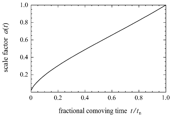
Figure 1: Scale factor $a(t)$ versus fractional comoving time $t/t_{\rm n}$. It turns out that the expansion history of this model matches closely the observed one.

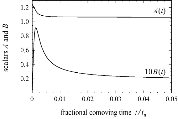
Figure 2: Time dependence of the scalars $A$ and $B$. At late times, the scalars approach constant values.

Such a spacetime variation of $A$ and $B$ has various implications for the scalars themselves and (due to the coupling of $A$ and $B$ to $F^{\mu\nu}$) for electrodynamics. These implications are discussed in Secs. 4 and 5, respectively.

4 Effects in the scalar sector

To gain insight into how the time-dependent cosmological background solutions $A_{\rm b}$ and $B_{\rm b}$ affect the scalars themselves, we investigate the propagation properties of small localized excitations $\delta A$ and $\delta B$ of the cosmological background $A_{\rm b}$ and $B_{\rm b}$. For such a study, it is appropriate to work in local coordinates, which we take to be anchored at the spacetime point $x_{0}$.

Substituting the ansatz

$$A(x) = A_{\rm b}(x)+\delta A(x)$$

$$B(x) = B_{\rm b}(x)+\delta B(x)$$ (9)

for the scalars into the equations of motion for $A$ and $B$ determines the dynamics of the perturbations $\delta A$ and $\delta B$. One obtains the following linearized equations:

$${}\!\!\!0 = \big{[}\Box-2B^{\mu}\partial_{\mu}+2m_{A}^{2}B_{\rm b}^{2}\big{]}\delta A-\big{[}2A^{\mu}\partial_{\mu}-2A^{\mu}B_{\mu}-4m_{A}^{2}A_{\rm b}B_{\rm b}\big{]}\delta B\;,$$

$$0 = \big{[}2A^{\mu}\partial_{\mu}\big{]}\delta A+\big{[}\Box-2B^{\mu}\partial_{\mu}+6m_{B}^{2}B_{\rm b}^{2}-A^{\mu}A_{\mu}+B^{\mu}B_{\mu}\big{]}\delta B\;.$$ (10)

Here, $A_{\rm b}$ and $B_{\rm b}$ as well as $A^{\mu}\equiv B_{\rm b}^{-1}\partial^{\mu}A_{\rm b}$, and $B^{\mu}\equiv B_{\rm b}^{-1}\partial^{\mu}B_{\rm b}$ are evaluated at $x=x_{0}$.

Equation (10) determines the propagation features of $\delta A$ and $\delta B$ in the varying cosmological background. In the context of this equation, $A^{\mu}$ and $B^{\mu}$ are external nondynamical vectors selecting a preferred direction in the local inertial frame. It follows that the propagation of $\delta A$ and $\delta B$ in the varying cosmological background fails to obey Lorentz symmetry. This result carries over to quantum theory: the traveling disturbances $\delta A$ and $\delta B$ would be seen as the effective particles corresponding to the scalars $A$ and $B$, so that such particles would violate Lorentz invariance.

We remark that the usual ansatz with $\exp(-ip\cdot x)$ yields the plane-wave dispersion relation. As expected, this dispersion relation contains the fixed vectors $A^{\mu}$ and $B^{\mu}$ contracted with the momentum $p^{\mu}$ implying Lorentz breaking. In addition, this dispersion relation exhibits imaginary terms leading to decaying solutions. This is consistent with the nonconservation of 4-momentum due to the violation of translational invariance. We also point out that the equations of motion are coupled, so that a plane-wave is a linear combination of $\delta A$ and $\delta B$. More details can be found in Ref. blpr.

5 Effects in the scalar-coupled sector

Instead of excitations $\delta A$ and $\delta B$ of the scalar fields, we now consider excitations of $F_{\mu\nu}$ in our background cosmological solution $A_{\rm b}$ and $B_{\rm b}$. Again, it is appropriate to work in a local inertial frame. Then, the effective Lagrangian ${\mathcal{L}}_{\rm cosm}$ for localized $F_{\mu\nu}$ fields follows from Eq. (3)

$${\mathcal{L}}_{\rm cosm}=-{\textstyle{{1}\over{4}}}M_{\rm b}F_{\mu\nu}F^{\mu\nu}-{\textstyle{{1}\over{4}}}N_{\rm b}F_{\mu\nu}\tilde{F}^{\mu\nu}\;,$$ (11)

where $M_{\rm b}$ and $N_{\rm b}$ are determined by the time-dependent cosmological solutions $A_{\rm b}$ and $B_{\rm b}$ for the scalars.

The physics content of ${\mathcal{L}}_{\rm cosm}$ is best extracted by comparison to the conventional electrodynamics Lagrangian ${\mathcal{L}}_{\rm em}$ given by

$${\mathcal{L}}_{\rm em}=-{{1}\over{4e^{2}}}F_{\mu\nu}F^{\mu\nu}-{{\theta}\over{16\pi^{2}}}F_{\mu\nu}\tilde{F}^{\mu\nu}\;.$$ (12)

This shows that $e^{2}\equiv 1/M_{\rm b}$ and $\theta\equiv 4\pi^{2}N_{\rm b}$. Since $M_{\rm b}$ and $N_{\rm b}$ are functions of the varying scalar background $A_{\rm b}$ and $B_{\rm b}$, the electromagnetic couplings $e$ and $\theta$ are no longer constant in general. In other words, in our supergravity cosmology the fine-structure parameter $\alpha$ and the electromagnetic $\theta$ angle acquire related spacetime dependences. The evolution of $\alpha$ in the present model with initial conditions (8) is depicted in Fig. 3. Also shown is the recently reported Webb dataset[32] obtained from measurements of high-redshift spectra.

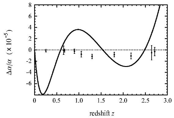
Figure 3: Relative change in the fine-structure parameter $\alpha$ versus redshift. For comparison, the Webb data has been included into the plot. Although disagreeing in detail, the data and the model exhibit variations of $\alpha$ of roughly the same order of magnitude.

Lorentz violation in our effective electrodynamics can be clearly established by inspection of the modified Maxwell equations resulting from the Lagrangian (11):

$${{1}\over{e^{2}}}\partial^{\mu}F_{\mu\nu}-{{2}\over{e^{3}}}(\partial^{\mu}e)F_{\mu\nu}+{{1}\over{4\pi^{2}}}(\partial^{\mu}\theta)\tilde{F}_{\mu\nu}=0\;.$$ (13)

In our supergravity cosmology, the gradients of $e$ and $\theta$ appearing in Eq. (13) are nonzero, approximately constant in local inertial frames, and act as a nondynamical external background. This vectorial background selects a preferred direction in the local inertial frame violating Lorentz symmetry.

We remark that the term exhibiting the gradient of $\theta$ can be identified with a Chern–Simons-type contribution to the modified Maxwell equations. Such a term, which is contained in the minimal SME, has received a lot of attention recently.[33] For example, it typically leads to vacuum Čerenkov radiation.[34]

6 Summary

In this talk, it has been demonstrated that the violation of spacetime-translation invariance is closely intertwined with the breaking of Lorentz symmetry. More specifically, a varying scalar—regardless of the mechanism driving the variation—is associated with a nonzero gradient, which selects a preferred direction in spacetime. This mechanism for Lorentz violation is interesting because varying scalars appear in many cosmological contexts.

References

- [1] For an overview see, e.g., CPT and Lorentz Symmetry II, edited by V.A. Kostelecký (World Scientific, Singapore, 2002).
- [2] V.A. Kostelecký and S. Samuel, Phys. Rev. D 39, 683 (1989); Phys. Rev. Lett. 63, 224 (1989); 66, 1811 (1991); V.A. Kostelecký and R. Potting, Nucl. Phys. B 359, 545 (1991); Phys. Lett. B 381, 89 (1996); Phys. Rev. D 63, 046007 (2001); V.A. Kostelecký et al., Phys. Rev. Lett. 84, 4541 (2000).
- [3] G. Amelino-Camelia et al., Nature (London) 393, 763 (1998).
- [4] D. Sudarsky et al., Phys. Rev. D 68, 024010 (2003).
- [5] F.R. Klinkhamer, Nucl. Phys. B 578, 277 (2000).
- [6] J. Alfaro et al., Phys. Rev. Lett. 84, 2318 (2000); Phys. Rev. D 65, 103509 (2002).
- [7] S.M. Carroll et al., Phys. Rev. Lett. 87, 141601 (2001); Z. Guralnik et al., Phys. Lett. B 517, 450 (2001); A. Anisimov et al., Phys. Rev. D 65, 085032 (2002); C.E. Carlson et al., Phys. Lett. B 518, 201 (2001).
- [8] D. Colladay and V.A. Kostelecký, Phys. Rev. D 55, 6760 (1997); 58, 116002 (1998); V.A. Kostelecký and R. Lehnert, Phys. Rev. D 63, 065008 (2001); V.A. Kostelecký, Phys. Rev. D 69, 105009 (2004).
- [9] KTeV Collaboration, H. Nguyen, in Ref. \refcitecpt01; OPAL Collaboration, R. Ackerstaff et al., Z. Phys. C 76, 401 (1997); DELPHI Collaboration, M. Feindt et al., preprint DELPHI 97-98 CONF 80 (1997); BELLE Collaboration, K. Abe et al., Phys. Rev. Lett. 86, 3228 (2001); BaBar Collaboration, B. Aubert et al., hep-ex/0303043; FOCUS Collaboration, J.M. Link et al., Phys. Lett. B 556, 7 (2003).
- [10] V.A. Kostelecký and R. Potting, Phys. Rev. D 51, 3923 (1995).
- [11] D. Colladay and V.A. Kostelecký, Phys. Lett. B 344, 259 (1995); Phys. Rev. D 52, 6224 (1995); V.A. Kostelecký and R. Van Kooten, Phys. Rev. D 54, 5585 (1996); O. Bertolami et al., Phys. Lett. B 395, 178 (1997); N. Isgur et al., Phys. Lett. B 515, 333 (2001).
- [12] V.A. Kostelecký, Phys. Rev. Lett. 80, 1818 (1998); Phys. Rev. D 61, 016002 (2000); Phys. Rev. D 64, 076001 (2001).
- [13] D. Bear et al., Phys. Rev. Lett. 85, 5038 (2000); D.F. Phillips et al., Phys. Rev. D 63, 111101 (2001); M.A. Humphrey et al., Phys. Rev. A 68, 063807 (2003); Phys. Rev. A 62, 063405 (2000); V.A. Kostelecký and C.D. Lane, Phys. Rev. D 60, 116010 (1999); J. Math. Phys. 40, 6245 (1999).
- [14] R. Bluhm et al., Phys. Rev. Lett. 88, 090801 (2002).
- [15] F. Canè et al., Phys. Rev. Lett. 93, 230801 (2004).
- [16] H. Dehmelt et al., Phys. Rev. Lett. 83, 4694 (1999); R. Mittleman et al., Phys. Rev. Lett. 83, 2116 (1999); G. Gabrielse et al., Phys. Rev. Lett. 82, 3198 (1999); R. Bluhm et al., Phys. Rev. Lett. 82, 2254 (1999); Phys. Rev. Lett. 79, 1432 (1997); Phys. Rev. D 57, 3932 (1998).
- [17] B. Heckel, in Ref. \refcitecpt01; L.-S. Hou et al., Phys. Rev. Lett. 90, 201101 (2003); R. Bluhm and V.A. Kostelecký, Phys. Rev. Lett. 84, 1381 (2000).
- [18] H. Müller et al., Phys. Rev. D 68, 116006 (2003); R. Lehnert, Phys. Rev. D 68, 085003 (2003); J. Math. Phys. 45, 3399 (2004); Int. J. Mod. Phys. A 20, 1303 (2005).
- [19] S.M. Carroll et al., Phys. Rev. D 41, 1231 (1990); V.A. Kostelecký and M. Mewes, Phys. Rev. Lett. 87, 251304 (2001); Phys. Rev. D 66, 056005 (2002); J. Lipa et al., Phys. Rev. Lett. 90, 060403 (2003); H. Müller et al., Phys. Rev. Lett. 91, 020401 (2003); Phys. Rev. D 67, 056006 (2003); V.A. Kostelecký and A.G.M. Pickering, Phys. Rev. Lett. 91, 031801 (2003); G.M. Shore, Contemp. Phys. 44, 503 (2003); P. Wolf et al., Gen. Rel. Grav. 36, 2352 (2004); Q. Bailey and V.A. Kostelecký, Phys. Rev. D 70, 076006 (2004).
- [20] V.W. Hughes et al., Phys. Rev. Lett. 87, 111804 (2001); R. Bluhm et al., Phys. Rev. Lett. 84, 1098 (2000); E.O. Iltan, JHEP 0306, 016 (2003).
- [21] E.O. Iltan, Mod. Phys. Lett. A 19, 327 (2004); D.L. Anderson et al., Phys. Rev. D 70, 016001 (2004).
- [22] S. Coleman and S.L. Glashow, Phys. Rev. D 59, 116008 (1999); V. Barger et al., Phys. Rev. Lett. 85, 5055 (2000); J.N. Bahcall et al., Phys. Lett. B 534, 114 (2002); V.A. Kostelecký and M. Mewes, Phys. Rev. D 70, 031902 (2004).
- [23] V.A. Kostelecký and M. Mewes, Phys. Rev. D 69, 016005 (2004).
- [24] E. Cremmer and J. Scherk, Nucl. Phys. B 118, 61 (1977); P. Forgacs and Z. Horvath, Gen. Rel. Grav. 11, 205 (1979); A. Chodos and S. Detweiler, Phys. Rev. D 21, 2167 (1980); W.J. Marciano, Phys. Rev. Lett. 52, 489 (1984); T. Damour and A.M. Polyakov, Nucl. Phys. B 423, 532 (1994).
- [25] R.R. Caldwell et al., Phys. Rev. Lett. 80, 1582 (1998); A. Masiero et al., Phys. Rev. D 61, 023504 (2000); Y. Fujii, Phys. Rev. D 62, 044011 (2000).
- [26] C. Armendáriz-Picón et al., Phys. Lett. B 458, 209 (1999).
- [27] A.H. Guth, Phys. Rev. D 23, 347 (1981).
- [28] E. Cremmer and B. Julia, Nucl. Phys. B 159, 141 (1979).
- [29] V.A. Kostelecký et al., Phys. Rev. D 68, 123511 (2003).
- [30] A. Das et al., Phys. Rev. D 16, 3427 (1977).
- [31] O. Bertolami et al., Phys. Rev. D 69, 083513 (2004).
- [32] J.K. Webb et al., Phys. Rev. Lett. 82, 884 (1999); 87, 091301 (2001).
- [33] R. Jackiw and V.A. Kostelecký, Phys. Rev. Lett. 82, 3572 (1999); C. Adam and F.R. Klinkhamer, Nucl. Phys. B 657, 214 (2003); H. Belich et al., Phys. Rev. D 68, 025005 (2003); M.B. Cantcheff et al., Phys. Rev. D 68, 065025 (2003); B. Altschul, Phys. Rev. D 69, 125009 (2004).
- [34] R. Lehnert and R. Potting, Phys. Rev. Lett. 93, 110402 (2004); Phys. Rev. D 70, 125010 (2004) [Erratum-ibid. D 70, 129906 (2004)]; see also these proceedings.