Quantum Gravity: General Introduction and Recent Developments

Abstract.

I briefly review the current status of quantum gravity. After giving some general motivations for the need of such a theory, I discuss the main approaches in quantizing general relativity: Covariant approaches (perturbation theory, effective theory, and path integrals) and canonical approaches (quantum geometrodynamics, loop quantum gravity). I then address quantum gravitational aspects of string theory. This is followed by a discussion of black holes and quantum cosmology. I end with some remarks on the observational status of quantum gravity.

1. Why quantum gravity?

The consistent implementation of the gravitational interaction into the quantum framework is considered to be the outstanding problem in fundamental physics. A big obstacle so far is the lack of a direct experimental hint. Therefore, the motivations for the need of such a theory are at present purely theoretical. These motivations strongly indicate, however, that the present framework of theoretical physics is incomplete. In the following I shall briefly discuss the main reasons that motivate the search for a quantum theory of gravity. More details on this as well as on the other issues discussed in this review can be found in my monograph [1] to which I refer the reader for more details and references.

Why should one believe that there is a need for a quantum theory of gravity?

• Singularity theorems: Under very general conditions, it follows from general relativity (GR) that singularities in spacetime are unavoidable [2]. GR, therefore, predicts its own breakdown. This applies in particular to the universe as a whole: there are strong indications for the presence of an initial singularity (this can be inferred from the existence of the cosmic microwave background radiation). Since the classical theory is then no longer applicable, a more comprehensive theory must be found – the general expectation is that this is a quantum theory of gravity.

• Initial conditions in cosmology: This is related to the first point. Cosmology as such is incomplete if its beginning cannot be described in physical terms. It seems that even an inflationary epoch cannot avoid a singularity in the past [3]. Inflation itself is based on the ‘no-hair conjecture’ according to which spacetime approaches locally de Sitter space if a positive (effective) cosmological constant is present. An implicit assumption for the validity of the no-hair conjecture is that modes smaller than the Planck scale (see below) are not excited to macroscopic scales (‘trans-Planckian problem’).

• Evolution of black holes: Black holes radiate with a temperature proportional to $\hbar$, the Hawking temperature [2], see below. For the final evaporation, a full theory of quantum gravity is needed since the semiclassical approximation leading to the Hawking temperature then breaks down.

• Unification of all interactions: All non-gravitational interactions have so far been successfully accomodated into the quantum framework. Gravity couples universally to all forms of energy. One would therefore expect that in a unified theory of all interactions, also gravity is described in quantum terms.

• Inconsistency of an exact semiclassical theory: All attempts to construct a fundamental theory where a classical gravitational field is coupled to quantum fields have failed up to now [1]. Such a semiclassical theory seems to exist only in an approximate sense.

• Avoidance of divergences: It has long been speculated that quantum gravity may lead to a theory devoid of the ubiquitous divergences arising in quantum field theory. This may happen, for example, through the emergence of a natural cutoff at small distances (large momenta). In fact, modern approaches such as string theory or loop quantum gravity (see below) provide indications for a discrete structure at small scales.

At which scale(s) would one expect that effects of quantum gravity necessarily occur? As shown by Max Planck in 1899, gravitational constant $G$, quantum of action $\hbar$ and speed of light $c$ can be combined in a unique way (apart from numerical factors) to provide fundamental units of length, time, and mass, respectively. These ‘Planck units’ read

$$l_{\rm P} = \sqrt{\frac{\hbar G}{c^{3}}}\approx 1.62\times 10^{-33}\,{\rm cm}\ ,$$ (1)

$$t_{\rm P} = \sqrt{\frac{\hbar G}{c^{5}}}\approx 5.40\times 10^{-44}\,{\rm s}\ ,$$ (2)

$$m_{\rm P} = \sqrt{\frac{\hbar c}{G}}\approx 2.17\times 10^{-5}\,{\rm g}\approx 1.22\times 10^{19}\,{\rm GeV}\ .$$ (3)

One might think that the presence of a fundamental length scale is not a Lorentz invariant notion. This is, however, not necessarily the case because special relativity cannot be applied in this regime and, moreover, lengths should be related to eigenvalues of a geometric quantum operator, cf. [4] for a detailed discussion in the framework of loop quantum gravity.

Quantization of gravity means quantization of geometry. But which structures should be quantized, that is, to which structures should one apply the superposition principle? Chris Isham has presented the hierarchy of structures depicted in Fig. 1 [5].

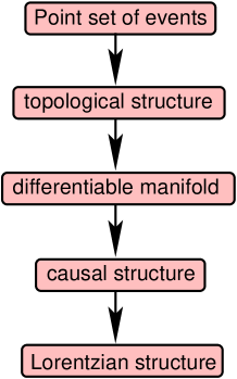
Figure 1. Different levels for the application of quantization

Structures that are not quantized remain as absolute (non-dynamical) entities in the formalism. One would expect that in a fundamental theory no absolute structure remains. This is referred to as background independence of the theory.

Problem of time

A particular aspect of background independence is the ‘problem of time’, which arises in any approach to quantum gravity. On the one hand, time is external in ordinary quantum theory; the parameter $t$ in the Schrödinger equation,

$${\rm i}\hbar\,\frac{\partial\psi}{\partial t}=H\psi\ ,$$ (4)

is identical to Newton’s absolute time—it is not turned into an operator and is presumed to be prescribed from the outside. This is true also in special relativity where the absolute time $t$ is replaced by Minkowski spacetime, which is again an absolute structure.

On the other hand, time in general relativity is dynamical because it is part of spacetime described by Einstein’s equations,

$$R_{\mu\nu}-\frac{1}{2}\,g_{\mu\nu}\,R+\Lambda g_{\mu\nu}=\frac{8\pi G}{c^{4}}T_{\mu\nu}\ .$$ (5)

Both concepts cannot be true fundamentally. It is expected that the fundamental theory does not contain any absolute structure. We shall see below how far present approaches to quantum gravity implement background independence.

Hawking effect

The relationship between quantum theory and gravity has been experimentally investigated only on the level of Newtonian gravity implemented into the Schrödinger equation or its relativistic generalizations, cf. [6] for a recent review. On the level of quantum field theory on a classical gravitational background there exists a specific prediction which has, however, not yet been tested: Black holes radiate with a temperature proportional to $\hbar$ (‘Hawking radiation’),

$$T_{\rm BH}=\frac{\hbar\kappa}{2\pi k_{\rm B}c}\ ,$$ (6)

where $\kappa$ is the surface gravity. For a Schwarzschild black hole this yields

$$T_{\rm BH}=\frac{\hbar c^{3}}{8\pi k_{\rm B}GM}\approx 6.17\times 10^{-8}\left(\frac{M_{\odot}}{M}\right)\ {\rm K}\ .$$ (7)

The black hole shrinks due to Hawking radiation and possesses a finite lifetime. The final phase, where $\gamma$-radiation is being emitted, could be observable. The temperature (7) is unobservably small for black holes that result from stellar collapse. One would need primordial black holes produced in the early universe because they could possess a sufficiently low mass [7]. For example, black holes with an initial mass of $5\times 10^{14}$ g would evaporate at the present age of the universe. In spite of several attempts, no experimental hint for black-hole evaporation has been found. Primordial black holes can result from density fluctuations produced during an inflationary epoch [7]. However, they can only be produced in sufficient numbers if the scale invariance of the power spectrum is broken at some scale, cf. [8].

Since black holes radiate thermally, they also possess an entropy, the ‘Bekenstein–Hawking entropy’, which is given by the expression

$$S_{\rm BH}=\frac{k_{\rm B}c^{3}A}{4G\hbar}=k_{\rm B}\frac{A}{4l_{\rm P}^{2}}\ ,$$ (8)

where $A$ is the surface area of the event horizon. For a Schwarzschild black hole with mass $M$, this reads

$$S_{\rm BH}\approx 1.07\times 10^{77}k_{\rm B}\left(\frac{M}{M_{\odot}}\right)^{2}\ .$$ (9)

Since the Sun has an entropy of about $10^{57}k_{\rm B}$, this means that a black hole resulting from the collapse of a star with a few solar masses would experience an increase in entropy by twenty orders of magnitude during its collapse.

It is one of the challenges of any approach to provide a microscopic explanation for this entropy, that is, to derive (8) from a counting of microscopic quantum gravitational states.

Main Approaches

What are the main approaches?

• Quantum general relativity: The most straightforward attempt, both conceptually and historically, is the application of ‘quantization rules’ to classical general relativity. One distinguishes

  • Covariant approaches: These are approaches that employ four-dimensional covariance at some stage of the formalism. Examples include perturbation theory, effective field theories, renormalization-group approaches, and path integral methods.

  • Canonical approaches: Here one makes use of a Hamiltonian formalism and identifies appropriate canonical variables and conjugate momenta. Examples include quantum geometrodynamics and loop quantum gravity.

• String theory: This is the main approach to construct a unifying quantum framework of all interactions. The quantum aspect of the gravitational field only emerges in a certain limit in which the different interactions can be distinguished.

• There are a couple of other attempts such as quantization of topology, or the theory of causal sets, which I will not address in this short review.

2. Covariant quantization

Perturbative Quantum Gravity

Historically, the first attempt to quantize gravity was through perturbation theory. In 1930, Léon Rosenfeld investigated the gravitational field produced by an electromagnetic field and calculated the gravitational self-energy after quantization [9]. It turned out to be infinite. Infinities have been encountered before in the self-energy of the electron, and Rosenfeld did his calculation (following a question by Werner Heisenberg) to see whether such infinities already occur in situations where only ‘fields’ (no ‘matter fields’ such as electrons) are present.

Perturbation theory starts by decomposing the metric, $g_{\mu\nu}$, into a background part, $\bar{g}_{\mu\nu}$, and a ‘small’ perturbation, $f_{\mu\nu}$,

$$g_{\mu\nu}=\bar{g}_{\mu\nu}+\sqrt{32\pi G}f_{\mu\nu}\ .$$ (10)

The important assumption is the presence of an (approximate) background with respect to which standard perturbation theory (formulation of Feynman rules, etc.) can be applied. In this approximate framework the quantum aspects of gravity are encoded in a spin-2 particle propagating on the background – the graviton. In contrast to Yang–Mills theory, however, the ensuing perturbation theory is non-renormalizable: At each order in the expansion with respect to $G$, new types of divergences occur which have to be absorbed into appropriate parameters that have to be fixed by measurement. All together, one would have to introduce infinitely many parameter, rendering the theory useless. An explicit calculation of the 2–loop divergence in 1985 has shown that the divergences are real and that there is no ‘miraculous’ cancellation of divergences already in the absence of non-gravitational fields [10]. The corresponding divergent two-loop Lagrangian reads

$${\mathcal{L}}^{({\rm div})}_{\rm 2-loop}=\frac{209\hbar^{2}}{2880}\,\frac{32\pi G}{(16\pi^{2})^{2}\epsilon}\,\bar{R}^{\alpha\beta}{}_{\gamma\delta}\,\bar{R}^{\gamma\delta}{}_{\mu\nu}\,\bar{R}^{\mu\nu}{}_{\alpha\beta}\ ,$$ (11)

where $\epsilon$ is a regularization parameter (from dimensional regularization) that goes to zero and thus produces a divergence. The presence of supersymmetry (SUSY) alleviates the occurrence of divergences; they, however, appear at higher loops and thus do not seem to prevent the theory from being perturbatively non-renormalizable.

Effective Field Theories and Renormalization Group

Even if the theory is perturbatively non-renormalizable, it may lead to definite predictions at low energies. This is the framework of ‘effective field theories’. As an example I quote the quantum gravitational correction to the Newtonian potential, calculated in [11],

$$V(r)=-\frac{Gm_{1}m_{2}}{r}\,\left(1+3\frac{G(m_{1}+m_{2})}{2r}+\frac{41}{10\pi}\,\frac{G\hbar}{r^{2}}\right)\ .$$ (12)

This result is independent of the ambiguities that are present at higher energies. In fact, effective field theories are successfully applied elsewhere, for example, ‘chiral perturbation theory’ in QCD (where one considers the limit of the pion mass $m_{\pi}\to 0$) is such an effective theory.

A theory that is perturbatively non-renormalizable may still be non-perturbatively renormalizable. A standard example is the three-dimensional Gross–Neveu model with a large number of flavour components [12]. Could this happen for quantum general relativity, too? A theory may be ‘asymptotically safe’ in the sense that a non-Gaussian (non-vanishing) ultraviolet (UV) fixed point exists non-perturbatively [13]. In fact, there are indications that this is the case [14]: Consider an ‘Einstein–Hilbert truncation’ defined by the action (in $d$ spacetime dimensions)

$$\Gamma_{k}[g]=\frac{1}{16\pi G_{k}}\,\int{\rm d}^{d}x\,\sqrt{g}\,\left(-R(g)+2\bar{\lambda}_{k}\right)\,,$$ (13)

plus classical gauge fixing, where $\bar{\lambda}_{k}$ and $G_{k}$ are the momentum ($k$-) dependent cosmological and gravitational constant, respectively. Studying the renormalization-group equations within this truncation (which is of course a very restrictive ansatz), it is found in [14] that the dimensionless versions of these parameters, $\lambda_{k}=k^{-2}\bar{\lambda}_{k}$ and $g_{k}=k^{d-2}G_{k}$, have an UV attractive non-Gaussian fixed point at values $(\lambda_{*},g_{*})\neq(0,0)$. Therefore, as $k\to\infty$,

$$G_{k}\approx\frac{g_{*}}{k^{d-2}}\,,\quad\bar{\lambda}\equiv\Lambda\approx\lambda_{*}\,k^{2}\ .$$ (14)

The gravitational constant thus vanishes in this limit (for $d>2$), and the theory would be asymptotically free. Using more general truncations, it may also be possible to obtain a small positive cosmological constant as a strong infrared quantum effect [15] and to get a growth of $G$ at large distances which could explain the observed flat galaxy rotation curves [16]. Although these results have been obtained within special truncations and may not survive in the full theory, they show that quantum GR could in principle be perturbatively renormalizable and lead to testable predictions even at a macroscopic level (and what could be more macroscopic than galaxies). This is also the hope for the approaches to quantum GR presented below.

Path Integrals

In quantum mechanics and quantum field theory, path integrals provide a convenient tool for a wide range of applications. Among them are saddle point approximations and non-perturbative approaches, the latter typically in a lattice framework. In quantum gravity, a path-integral formulation would have to employ a sum over all four-metrics for a given topology,

$$Z[g]=\int{\mathcal{D}}g_{\mu\nu}(x)\,{\rm e}^{{\rm i}S[g_{\mu\nu}(x)]/\hbar}\ .$$ (15)

In addition, one would expect that a sum over all topologies has to be performed. Since four-manifolds are not classifiable, this is an impossible task. Attention is therefore restricted to a given topology (or to a sum over few topologies). Still, the evaluation of an expression such as (15) meets great mathematical and conceptual difficulties.

From a methodological point of view, one distinguishes between a Euclidean and a Lorentzian version of the path integral (15). In the Euclidean version, one performs a Wick rotation $t\to-{\rm i}\tau$ in the action and integrates over Euclidean metrics only. In ordinary quantum field theory, this improves the convergence properties of the path integral. In quantum gravity, however, the situation is different because the Euclidean action is unbounded from below. This unboundedness is not necessarily a problem as long as one is only concerned with a saddle point approximation of the path integral, that is, a WKB aproximation of the form $\exp(-I)$, where $I$ denotes the extremal value of the Euclidean action.

Such an approximation lies, in fact, at the heart of one of the prominent proposals for boundary conditions in quantum cosmology—the ‘no-boundary condition’ or ‘Hartle–Hawking proposal’ [17]. This consists of two parts. First, it is assumed that the Euclidean form of the path integral is fundamental, and that the Lorentzian structure of the world only emerges in situations where the saddle point is complex. Second, it is assumed that one integrates over metrics with one boundary only (the boundary corresponding to the present universe), so that no ‘initial’ boundary is present; this is the origin of the term ‘no-boundary proposal’. The absence of an initial boundary is implemented through appropriate regularity conditions. In the simplest situation, one finds as the dominating geometry the ‘Hartle–Hawking instanton’ depicted in Fig. 2: the dominating contribution at small radii is (half of the) Euclidean four-sphere $S^{4}$, whereas for bigger radii it is (part of) de Sitter space, which is the analytic continuation of $S^{4}$. Both geometries are matched at a three-geometry with vanishing extrinsic curvature. The Lorentzian nature of our universe would thus only be an ‘emergent’ phenomenon.

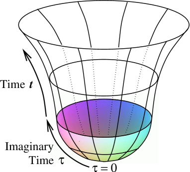
Figure 2. Hartle–Hawking instanton: The dominating contribution to the Euclidean path integral is assumed to be half of a four-sphere attached to a part of de Sitter space.

In more general situations, one has to look for integration contours in the space of complex metrics that render the integral convergent. Consider one quantum cosmological example discussed in detail in [18]. It describes a scalar field (called $\chi$ after a field redefinition) conformally coupled to the scale factor, $a$, of a Friedmann universe. The classical solutions are confined to a rectangle centred around the origin in the $(a,\chi)$-plane. One can explicitly construct wave packets that follow these classical trajectories. (They are solutions of the Wheeler–DeWitt equation discussed below.) The corresponding quantum states are normalizable in both the $a$ and the $\chi$ direction. A general quantum gravitational (cosmological) path integral depends on two values for $a$ and $\chi$, called $a^{\prime},a^{\prime\prime}$ and $\chi^{\prime},\chi^{\prime\prime}$. respectively. Fig. 3 shows the corresponding $(a^{\prime\prime},\chi^{\prime\prime})$ space; the values for $a^{\prime}$ and $\chi^{\prime}$ define the origin of the ‘light cones’ depicted in the Figure by bullets.

The Hartle–Hawking wave function is obtained for $a^{\prime}=0=\chi^{\prime}$, that is, for the case when the light cones in Fig. 3 shrink to one cone centred at the origin. For this model, the path integral can be evaluated exactly. The investigation in [18] has shown that there is no contour for the path integration in the complex-metric plane that leads to a wave function which can be used in the construction of wave packets following the classical trajectories: the resulting wave functions either diverge along the ‘light cones’ or they diverge for large values of $a$ and $\chi$. The states are thus not normalizable, and it is not clear how they should be interpreted.

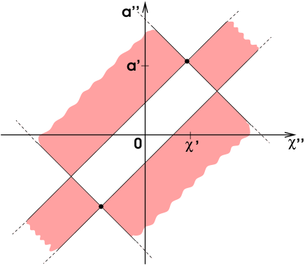
Figure 3. The wave functions obtained from the path integral for the model investigated in [18] either diverge along the light cones in minisuperspace or for large values of $a$ and $\chi$. They exhibit oscillatory behaviour in the shaded regions.

Dynamical triangulation

An alternative method to attack the full path integral (15) is dynamical triangulation, cf. [19] and the references therein. Here one starts from a Lorentzian path integral in the first place and employs a discretization of the geometry (a Euclidean formulation is used in an intermediate step of the calculations). In contrast to earlier attempts such as Regge calculus, the edge lengths of simplices are held fixed; the sum is then performed over all possible manifold gluings of equilateral simplices, using Monte Carlo simulations.

Some interesting results have already been obtained. First, the Hausdorff dimension $H$ of space, defined by $V(r)\propto\langle r\rangle^{H}$, where $V$ is the space volume, is found to read $H=3.10\pm 0.15$. This is an indication for the three-dimensionality of space (and thus for the four-dimensionality of spacetime). Since there is no background in quantum gravity, the dimension $d+1$ of the geometries to be summed over in the path integral does not need to be identical to the resulting value for $H+1$. Strangely enough, one had found earlier that for a Euclidean path integral the result is always $H=2$ for $d>2$. Second, a positive value for the cosmological constant, $\Lambda>0$, is needed. This is in accordance with results from recent measurements of the cosmic acceleration. However, no special value for $\Lambda$ seems to be preferred. Third, for large scales the volume seems to behave semiclassically. However, in spite of these promising hints, a continuum limit is still elusive.

3. Canonical quantization

One of the earliest attempts to quantize gravity employs a Hamiltonian approach. In a first step, the classical theory (GR) is reformulated in ‘3+1 form’ in which it describes the dynamics of three-geometries (with matter fields on them). Global hyperbolicity of the spacetime from which one starts is a necessary prerequisite. It must be emphasized that the topology of the three-dimensional space $\Sigma$ is fixed, that is, there is one canonical theory for each topology. In a second step, the canonical variables, that is, the configuration variable and its momentum (the ‘symplectic structure’) is chosen. The third step then addresses the canonical quantization procedure. The most straightforward approach would be to choose the three-metric and its conjugate momentum (which is a linear function of the second fundamental form). The resulting quantum theory is called ‘quantum geometrodynamics’ and is historically the oldest approach. More recently, alternative systems of variables have proved to be of great interest; because they can be interpreted as a connection or a loop variable, the corresponding approaches are called ‘quantum connection dynamics’ or ‘loop quantum gravity’. I shall review these approaches briefly in the following.

The central equations are the quantum constraints. The invariance of the classical theory under coordinate transformation leads to four (local) constraints: the Hamiltonian constraint,

$${\mathcal{H}}_{\bot}\Psi=0\ ,$$ (16)

and the three diffeomorphism (or momentum) constraints,

$${\mathcal{H}}_{a}\Psi=0\ .$$ (17)

The total gravitational Hamiltonian reads (apart from boundary terms)

$$H=\int{\rm d}^{3}x\ \left(N{\mathcal{H}}_{\bot}+N^{a}{\mathcal{H}}_{a}\right)\ ,$$ (18)

where $N$ (‘lapse function’) and $N^{a}$ (‘shift vector’) are Lagrange multipliers. In the connection and loop approaches, three additional (local) constraints emerge because of the freedom to choose the local triads upon which the formulation is based.

Some interesting features occur for 2+1-dimensional spacetimes [20] but I shall restrict myself in the following to the four-dimensional case.

Quantum geometrodynamics

The canonical variables are the three-dimensional metric, $h_{ab}(x)$, and its conjugate momentum. In this case one usually refers to (16) (or the full equation $H\Psi=0$) as the ‘Wheeler–DeWitt equation’. Here are some characteristics of this approach:

• The wave functional $\Psi$ depends on the three-dimensional metric, but because of (17) it is invariant under coordinate transformations on three-space.

• No external time parameter is present anymore – in this sense the theory is ‘timeless’. This also holds for the connection and loop approaches.

• Such constraints result from any theory that is classically reparametrization invariant, that is, a theory without background structure.

• The Wheeler–DeWitt equation is (locally) hyberbolic, and one can thereby define a local ‘intrinsic time’ distinguished by the sign in this wave equation.

• This approach is a candidate for a non-perturbative quantum theory of gravity. But even if it is superseded by a more fundamental theory at the Planck scale (such as superstring theory, see below), it should approximately be valid away from the Planck scale. The reason is that GR is then approximately valid, and the quantum theory from which it emerges in the WKB limit is quantum geometrodynamics.

Let us consider a simple example: a Friedmann universe with scale factor $a\equiv{\rm e}^{\alpha}$ containing a massive scalar field $\phi$. This is an interesting model for quantum cosmology (see below). In this case, the diffeomorphism constraints are identically fulfilled, and the Wheeler–DeWitt equation (16) reads

$$H\psi\equiv\left({G}\hbar^{2}\frac{\partial^{2}}{\partial\alpha^{2}}-\hbar^{2}\frac{\partial^{2}}{\partial\phi^{2}}+m^{2}\phi^{2}{\rm e}^{6\alpha}-\frac{{\rm e}^{4\alpha}}{{G}}\right)\psi(\alpha,\phi)=0\ .$$ (19)

This equation is simple enough to find solutions (at least numerically) and to study physical aspects such as the dynamics of wave packets and the semiclassical limit [1].

The semiclassical approximation can be conveniently discussed also for the full Wheeler–DeWitt equation, at least in a formal sense (i.e., treating functional derivatives as if they were ordinary derivatives and neglecting the problem of anomalies). The discussion is also connected to the question: Where does the imaginary unit in the (functional) Schrödinger equation come from [21]? The full Wheeler–DeWitt equation is real,

$$H\Psi=0\ ,$$ (20)

and one would also expect real solutions for $\Psi$. An approximate solution is found through a Born–Oppenheimer-type of scheme, in analogy to molecular physics. This is discussed at great length in [1]. The state then assumes the form

$$\Psi\approx\exp({\rm i}S_{0}[h]/\hbar)\,\psi[h,\phi]\ ,$$ (21)

where $h$ is an abbreviation for the three-metric, and $\phi$ stands for non-gravitational fields. In short, one has

• $S_{0}$ obeys the Hamilton–Jacobi equation for the gravitational field and thereby defines a classical spacetime which is a solution to Einstein’s equations (this order is formally similar to the recovery of geometrical optics from wave optics via the eikonal equation).

• $\psi$ obeys an approximate (functional) Schrödinger equation,

  $${\rm i}\hbar\,\underbrace{\nabla\,S_{0}\,\nabla\psi}_{\frac{\displaystyle\partial\psi}{\displaystyle\partial t}}\approx H_{\rm m}\,\psi\ ,$$ (22)

  where $H_{\rm m}$ denotes the Hamiltonian for the non-gravitational fields $\phi$. Note that the expression on the left-hand side of (22) is a shorthand notation for an integral over space, in which $\nabla$ stands for functional derivatives with respect to the three-metric. Semiclassical time $t$ is thus defined in this limit from the dynamical variables.

• The next order of the Born-Oppenheimer scheme yields quantum gravitational correction terms proportional to the inverse Planck mass squared, ${1}/{m_{\rm P}^{2}}$. The presence of such terms may in principle lead to observable effects, for example, in the anisotropy spectrum of the cosmic microwave background radiation.

The canonical formalism can also be extended to quantum supergravity [1, 22]. Its semiclassical approximation – recovery of the functional Schrödinger equation and calculation of quantum gravitational correction terms – has recently been performed in [23].

The Born–Oppenheimer expansion scheme distinguishes a state of the form (21) from its complex conjugate. In fact, in a generic situation both states will decohere from each other, that is, they will become dynamically independent [24]. This is a type of symmetry breaking, in analogy to the occurrence of parity violating states in chiral molecules. It is through this mechanism that the i in the Schrödinger equation emerges.

The recovery of the Schrödinger equation (22) raises an interesting issue. It is well known that the notion of Hilbert space is connected with the conservation of probability (unitarity) and thus with the presence of an external time (with respect to which the probability is conserved). The question then arises whether the concept of a Hilbert space is still required in the full theory where no external time is present. It could be that this concept makes sense only on the semiclassical level where (22) holds.

A major problem with quantum geometrodynamics is the lack of a precise mathematical framework for the full theory. This provides one with a motivation to look for alternatives.

Connection and loop dynamics

Instead of the metric formulation of the last subsection one can use a different set of variables, leading to the connection or the loop formulation. Detailed expositions can be found, for example, in [25, 26, 27], see also [1]. Starting point are the ‘new variables’ introduced by Abhay Ashtekar in 1986,

$$E_{i}^{a}(x) = \sqrt{h}\,e^{a}_{i}(x)\ ,$$ (23)

$$GA^{i}_{a}(x) = \Gamma^{i}_{a}(x)+{\beta}K^{i}_{a}(x)\ .$$ (24)

Here, $e^{a}_{i}(x)$ is the local triad (with $i$ being the internal index), $h$ is the determinant of the three-metric, $\Gamma^{i}_{a}(x)$ the spin connection, and $K^{i}_{a}(x)$ the second fundamental form. The parameter $\beta\in{\mathbb{C}}\backslash\{0\}$ denotes a quantization ambiguity similar to the $\theta$-parameter ambiguity in QCD and is called the ‘Barbero–Immirzi parameter’. The canonical pair of variables are the densitized triad $E_{i}^{a}(x)$ (this is the new momentum) and the connection $A^{i}_{a}(x)$ (the new configuration variable). They obey the Poisson-bracket relation

$$\{A^{i}_{a}(x),E_{j}^{b}(y)\}=8\pi{\beta}\delta^{i}_{j}\delta^{b}_{a}\delta(x,y)\ .$$ (25)

The use of this pair leads to what is called ‘connection dynamics’. One can rewrite the above constraints in terms of these variables and subject them to quantization. In addition, one has to treat the ‘Gauss constraint’ arising from the freedom to perform arbitrary rotations in the local triads.

The loop variables, on the other hand, are constructed from a non-local version of the connection. Consider a loop in the three-space $\Sigma$, see Fig. 4.

Figure 4. An oriented loop in the three-manifold $\Sigma$.

The fundamental loop variable is the holonomy $U[A,\alpha]$ defined as the path-ordered product

$$U[A,\alpha]={\mathcal{P}}\exp\left(G\int_{\alpha}A\right)\ .$$ (26)

The conjugate variable is the ‘flux’ of $E^{a}_{i}$ through a two-dimensional surface ${\mathcal{S}}$ in $\Sigma$.

Loop quantum gravity

A central concept in the formulation of loop quantum gravity is the spin-network basis. This is a complete orthonormal basis with respect to which all appropriate quantum states can be expanded. How is it defined? A spin network is a triple $S(\Gamma,\vec{j},\vec{N})$, where $\Gamma$ denotes a graph, $\vec{j}$ is a set of ‘spins’ (representations of SU(2)) that are attached to the curves forming the graph, and $\vec{N}$ denotes the chosen collection of basis elements at the nodes where the curves meet. A spin-network state is then

$$\Psi_{S}[A]=f_{S}(U_{1},\ldots,U_{n})\ ,$$ (27)

where $f$ is a ‘cylindrical function’ attributed to the graph, which is defined as a mapping from $[{\rm SU}(2)]^{n}$ (putting a holonomy on each curve) to ${\mathbb{C}}$. One can show that a natural Hilbert-space structure can be constructed on the kinematical level, that is, before the constraints (16) and (17) are imposed.

The introduction of the group SU(2)—and with it the algebra of angular momenta—introduces a discrete structure into the formalism. It is thus of interest to consider geometrical operators and discuss their spectrum with respect to the kinematical Hilbert space. As one may have expected, the spectrum turns out to be discrete. As one example I want to mention the quantization of area. Applying the ‘area operator’ $\hat{A}({\mathcal{S}})$ (whose classical analogue is the area of the two-dimensional surface ${\mathcal{S}}$) to a spin-network state one obtains

$$\hat{A}({\mathcal{S}})\Psi_{S}[A]=8\pi\beta l_{\rm P}^{2}\sum_{P\in S\cap{\mathcal{S}}}\sqrt{j_{P}(j_{P}+1)}\Psi_{S}[A]\ .$$ (28)

The points $P$ denote the intersections of the spin network with the surface, see Fig. 5 for an example with four curves.

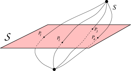
Figure 5. A spin network $S$ intersecting the surface $\mathcal{S}$.

Note that the area operator is not invariant under three-dimensional diffeomorphisms. This is because it is defined for an abstract surface in terms of coordinates. It does also not commute with the Hamiltonian constraint. An area operator that is invariant should be defined intrinsically with respect to curvature invariants or matter fields. A concrete realization of such an operator remains elusive.

In spite of much promising aspects, some open problems remain, cf. [28] and [25, 26]. They include:

• The presence of quantum anomalies in the constraint algebra could make the formalism inconsistent. How can anomalies be avoided?

• How does one have to treat the constraints? The Gauss constraint is easy to implement, but there are various subtleties and ambiguities with the diffeomorphism and Hamiltonian constraints.

• Can a semiclassical limit be obtained? Since the constraints assume now a form different from the one in geometrodynamics, a Born–Oppenheimer approach cannot be straightforwardly applied. An important role may be played by generalized coherent states. For large enough scales, the semiclassical approximations of loop quantum gravity and quantum geometrodynamics should of course coincide.

A path-integral formulation of loop quantum gravity employs the notion of ‘spin foam’, that is, time-developed spin networks that are integrated over, cf. [25] for details.

4. String theory

String theory (resp. M-theory) provides a drastically different approach to quantum gravity. The idea is to first construct a quantum theory of all interactions (a ‘theory of everything’) from which separate quantum effects of the gravitational field follow in some appropriate limit. String theory transcends local field theory in that it contains at the fundamental level higher dimensional objects (not only strings, but also branes) instead of points. However, as the discussion of loop quantum gravity above shows, non-local entities can also emerge in quantum GR. This is a consequence of background independence, which is not the case in standard field theories such as QED. A detailed exposition of this topic can be found in [29], cf. also [30] for a short non-technical overview. The main characteristics of string theory are:

• The appearance of gravity is inevitable. The graviton is an excitation of closed strings, and it appears via virtual closed strings in open-string amplitudes.

• String theory has as important ingredients the concepts of gauge invariance, supersymmetry (SUSY), and the presence of higher dimensions.

• It provides a unification of all interactions.

• String perturbation theory seems to be finite at each order, but the sum diverges.

• Only three fundamental constants are present: $\hbar,c$ and the string length $l_{\rm s}$; all other physical parameters (masses and coupling constants) should in principle be derivable from them.

• A net of dualities connects various string theories and indicates the presence of an underlying non-perturbative theory (M-theory) from which the various string theories can be recovered in appropriate limits.

Starting point is the formulation of a string action on the two-dimensional worldsheet of the string. It is given by the (generalized) Polyakov action describing the propagation of the string in a $D$-dimensional embedding (target) spacetime. For the bosonic string it reads

$$S\ \propto l_{\rm s}^{-2}\int{\rm d}^{2}\sigma\ \left(\sqrt{h}h^{\alpha\beta}\partial_{\alpha}X^{\mu}\partial_{\beta}X^{\nu}{g_{\mu\nu}(X)}\right.$$ (29)

$$\;\;\left.-l_{\rm s}^{2}\sqrt{h}\,{}^{(2)}\!R{\Phi(X)}+\epsilon^{\alpha\beta}\partial_{\alpha}X^{\mu}\partial_{\beta}X^{\nu}{B_{\mu\nu}(X)}\right)\ .$$

Here, $g_{\mu\nu}$ is the $D$-dimensional metric of the embedding space, $\Phi$ is the dilaton field, and $B_{\mu\nu}$ is an antisymmetric tensor field. They are all background fields, that is, they will not be integrated over in the path integral. In the path integral,

$$Z=\int{\mathcal{D}}X{\mathcal{D}}h\ {\rm e}^{-S}\ ,$$ (30)

one only integrates over the embedding variables $X^{\mu}$ (denoted here by $X$) and the worldsheet metric $h_{\alpha\beta}$ (denoted here by $h$). Note that one here usually employs a Euclidean path-integral formulation.

The path integral (30) contains in particular a sum over all worldsheets, that is, a sum over all Riemann surfaces. It is in this way that string interactions arise. One can then introduce a ‘string coupling’ constant $g$ that is related to the genus of the worldsheet—string perturbation theory is then an expansion with respect to $g$ (‘loop expansion’).

Demanding the absence of anomalies on the worldsheet leads to constraints:

• The background fields have to obey the ‘Einstein’s equations’ $+{\mathcal{O}}(l_{\rm s}^{2})$. They can be derived from an effective action, $S_{\rm eff}$, defined in the $D$-dimensional embedding space.

• The number of spacetime dimensions for the embedding space is restricted: One has $D=26$ for the bosonic string ($D=10$ resp. $D=11$ for the superstring).

There is an important connection between the worldsheet path integral and the effective action: Amplitudes for scattering processes (e.g. graviton–graviton scattering) calculated from string scattering are identical to the field-theoretic amplitudes of the corresponding processes which are derived from $S_{\rm eff}$ (they are found after a decomposition of the form (10) is made).

Apart from the lack of experimental evidence, there are various theoretical problems; they include

• There are many ways to compactify the additional spacetime dimensions (whose number is $D-4$). Moreover, these additionals dimensions may be non-compact as indicated by the existence of various ‘brane models’. Without a solution to this problem, no definite relation to low-energy coupling constants and masses can be made.

• Background independence is not yet fully implemented into string theory, as can be recognized from the prominent role of the embedding space. The AdS/CFT theories discussed in recent years may come close to background independence in some respect [31].

• The Standard Model of particle physics, which is experimentally extremely well tested, has not yet been recovered from string theory.

• What is M-theory and what is the role of the 11th dimension which has emerged in this context?

• Quantum cosmology has not yet been implemented into the full theory, only at the level of the effective action (‘string cosmology’).

Both string theory and loop quantum gravity exhibit aspects of non-commutative geometry. This could be relevant for understanding space at the smallest scale. In loop quantum gravity, the three-geometry is non-commutative in the sense that area operators of intersecting surfaces do not commute. In string theory, for $n$ coincident D-branes, the fields $X^{\mu}$ – the embeddings – and $A_{a}$ – the gauge fields – become non-commuting $n\times n$ matrices. It has also been speculated that time could emerge from a timeless framework if space were non-commutative [32]. This would be an approach very different from the recovery of time in quantum geometrodynamics discussed above. Quite generally, one envisages a highly non-trivial structure of space(time) in string theory [33].

5. Black holes

A major application for quantum gravity is black-hole physics. At the centre are two main questions. First, what happens at the final evaporation phase after the breakdown of Hawking’s semiclassical approximation? Second, how can one derive (8) in terms of quantum gravitational microstates? Whereas some results have been obtained concerning the entropy, an answer to the first question remains elusive. It has only indirectly been attacked in the form of the ‘information-loss problem’. I shall briefly discuss both issues in the following.

Black-hole entropy $S_{\rm BH}$?

A microscopic foundation of (8) has been attempted by both loop quantum gravity and string theory. Very briefly, the situation is as follows:

• Loop quantum gravity: The microscopic degrees of freedom are given by the spin-network states. An appropriate counting procedure for the number of the relevant horizon states leads to an entropy that is proportional to the Barbero–Immirzi parameter $\beta$. The demand for the result to be equal to (8) then fixes $\beta$. Until 2004, it was believed that the result is

  $$\beta=\frac{\ln 2}{\pi\sqrt{3}}\quad\left(\frac{\ln 3}{\pi\sqrt{2}}\right)\ ,$$ (31)

  where the value in parentheses would refer to the choice of SO(3) instead of SU(2). The SO(3)-value would have exhibited an interesting connection with the quasi-normal modes for the black hole. More recently, it was found that the original estimate for the number of states was too small. A new calculation yields the following numerical estimate for $\beta$ [34]: $\beta=0.237532\ldots$ An interpretation of this value at a more fundamental level has not yet been given.

• String theory: The microscopic degrees of freedom are here the D-branes, for which one can count the quantum states in the weak-coupling limit (where no black hole is present). Increasing the string coupling, one reaches a regime where no D-branes are present, but instead one has black holes. For black holes that are extremal in the relevant string-theory charges (for extremality the total charge is equal to the mass), the number of states is preserved (‘BPS black holes’), so the result for the black-hole entropy is the same as in the D-brane regime. In fact, the result is just (8), as it must be if the theory is consistent. This remains true for non-extremal black holes, but no result has been obtained for a generic black hole (say, an ordinary Schwarzschild black hole). More recently, an interesting connection has been found between the partition function, $Z_{\rm BH}$, for a BPS black hole and a topological string amplitude, $Z_{\rm top}$, [35],

  $$Z_{\rm BH}=|Z_{\rm top}|^{2}\ .$$ (32)

  Moreover, it has been speculated that the partition function can be identified with (the absolute square of) the Hartle–Hawking wave function of the universe discussed above [36]. This could give an interesting connection between quantum cosmology and string theory.

Information loss for black holes?

What happens during the final evaporation phase of a black hole? This is a major question for any theory of quantum gravity to answer. A definite answer is, however, elusive, and part of the discussion has circled around the ‘information-loss problem’ for black holes, see, for example, [37, 38]. What is the ‘information-loss problem’? According to Hawking’s semiclassical calculations, a black hole radiates with a thermal spectrum, with the temperature given by (6). As a consequence, the black hole loses mass and shrinks. In case that the hole completely evaporates and leaves only thermal radiation behind, any initial state for the black hole plus the quantum field would end with the same final state, which would be a thermal, that is, a mixed state. This would correspond to a maximal loss of information about the initial state. In other words: Unitarity would be violated for a closed system, in contrast to standard quantum theory.

Hawking originally argued that the final evaporation time, when the black hole has reached Planck-mass size and the semiclassical approximation breaks down, is too short for the original information to be recovered. Therefore, so his conclusion, there must be information loss in quantum gravity. More recently, Hawking has withdrawn his original opinion [39]. This switch is based on the argument that the full evolution is unitary if also components of the total wave function that do not evolve into a black hole are taken into account.

As we have seen, in full quantum gravity there is no notion of external time. However, for an isolated system such as a black hole, one can refer to the semiclassical time of external observers far away from the hole. The notion of unitarity then refers to this concept of time. So, if the fundamental theory of quantum gravity is unitary in this sense, there can be no information loss. Conversely, if the fundamental theory breaks unitarity in this sense, information loss is possible. As long as the situation with the full theory remains open, discussions of the information loss centre around assumptions and expectations.

However, for a black hole whose mass is much bigger than the Planck mass, the details of quantum gravity should be less relevant. It is of importance to emphasize that a (large) black hole is a macroscopic object. It is therefore strongly entangled with the quantum degrees of freedom with which it interacts. Information thereby becomes essentially non-local. This entanglement leads to decoherence for the black hole which thereby assumes classical properties analogously to other macroscopic objects [24]. In particular, the black hole itself does not evolve unitarily, cf. [40]. As was shown in [41], the interaction of the black hole with its Hawking radiation is sufficient to provide the black hole with classical behaviour; strictly speaking, the very notion of a black hole emerges through decoherence. The cases of a superposition of a black-hole state with its time-reversed version (a ‘white hole’) and with a no-hole state were considered and shown to decohere by Hawking radiation. This does not hold for virtual black holes, which are time symmetric and do not exhibit classical behaviour.

In the original derivation of Hawking radiation, one starts with a quantum field which is in its vacuum state. The thermal appearance of the resulting Hawking radiation is then recognized from the Planckian form of the expectation value of particle-number operator at late times. If the state of the quantum field is evaluated on a spatial hypersurface that enters the horizon, tracing out the degrees of freedom of the hole interior yields a thermal density matrix with temperature (6) in the outside region. (This is because the initial state of the field evolves into a two-mode squeezed state, and it is a general feature of such states that tracing out one mode leaves a thermal density matrix for the other mode.) However, one is not obliged to take a hypersurface that enters the horizon. One can consider a hypersurface that is locked at the bifurcation point (where the surface of the collapsing star crosses the horizon). Then, apart from its entanglement with the black hole itself, the field state remains pure. The observations far away from the hole should, however, not depend on the choice of the hypersurface [40]. This is, in fact, what results [42, 38]: The entanglement of the squeezed state representing the Hawking radiation with other (irrelevant) degrees of freedom leads to the thermal appearance of the field state. It therefore seems that there is no information-loss problem at the semiclassical level and that one can assume, at the present level of understanding, that the full evolution is unitary and that ‘information loss’ can be understood in terms of the standard dislocalization of information due to decoherence.

A similar point of view seems to emerge from discussions invoking string theory. In [43] it was argued that black holes are inherently associated with mixed states and that pure D-brane states rapidly experience decoherence due to entanglement with other degrees of freedom. An analogous situation (but without black holes) was discussed in [44]: Consider the decay of a massive string state. The decay spectrum of a single excited state does not show thermal behaviour. If one, however, averages over all the degenerate states with the same mass (justified by decoherence), the decay spectrum is Planckian. The authors of [45, 46] have argued that black-hole geometries result for a coarse-graining over smooth microstates. Quite generally, the thermodynamic properties of gravity seem to be a result of decoherence.

6. Quantum Cosmology

Why quantum cosmology?

Quantum cosmology is the application of quantum theory to the universe as a whole. Independent of any particular interaction, such a theory is needed in view of the extreme sensitivity of quantum system to their environment, that is, to other degrees of freedom [24]. However, since gravity is the dominating interaction on cosmic scales, a quantum theory of gravity is needed as a formal prerequisite for quantum cosmology.

Most work in quantum cosmology is based on the Wheeler–DeWitt equation of quantum geometrodynamics. The method is to restrict first the configuration space to a finite number of variables (scale factor, inflaton field, …) and then to quantize canonically. Since the full configuration space of three-geometries is called ‘superspace’, the ensuing models are called ‘minisuperspace models’. Eq. (19) is one special example describing a Friedmann universe with a massive scalar field. More recently, quantum cosmology was also discussed in the framework of loop quantum gravity. The following issues are typically addressed within quantum cosmology:

• How does one have to impose boundary conditions in quantum cosmology?

• Is the classical singularity being avoided?

• How does the appearance of our classical universe emerge from quantum cosmology?

• Can the arrow of time be understood from quantum cosmology?

• How does the origin of structure proceed?

• Is there a high probability for an inflationary phase?

• Can quantum cosmological results be justified from full quantum gravity?

In the following I shall briefly review only few aspects. More details can be found in [1] as well as in the reviews [47, 48, 49]. One particular proposal for boundary conditions in quantum cosmology, the Hartle–Hawking proposal, has alreay been addressed in Sect. 3.

Determinism of trajectories versus determinism of waves

One interesting aspect with far-reaching consequences is the following. The Wheeler–DeWitt equation (20) does not contain an external time parameter. Therefore, the quantum theory exhibits a kind of determinism drastically different from the classical theory [1]. Consider a model with a two-dimensional configuration space spanned by the scale factor, $a$, and a homogeneous scalar field, $\phi$, see Fig. 6. The classical model be such that there are solutions where the universe expands from an initial singularity, reaches a maximum, and recollapses to a final singularity. Classically, one would impose $a,\dot{a},\phi,\dot{\phi}$ (satisfying the constraint) at some $t_{0}$ (for example, at the left leg of the trajectory), and then the trajectory would be determined. This is indicated on the left-hand side of Fig. 6.

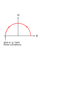
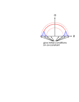
Figure 6. The classical and the quantum theory of gravity exhibit drastically different notions of determinism.

In the quantum theory, on the other hand, there is no $t$. The hyperbolic nature of (19) suggests to impose boundary conditions on $a=$ constant. In order to represent the classical trajectory by narrow wave packets, the ‘returning part’ of the packet must be present ‘initially’ (with respect to $a$). The determinism of the quantum theory then proceeds from small $a$ to large $a$, not along a classical trajectory (which does not exist). This behaviour has consequences for the validity of the semiclassical approximation and the arrow of time (see below).

Fate of classical singularity

Can quantum gravity avoid the classical singularities? So far no general criterium for singularity avoidance is available. An important question concerns the choice of an inner product which, for the quantum states in question, should be finite and conserved (with respect to some appropriate intrinsic time or, for example in black-hole cases, with respect to an external semiclassical time). Some examples include

• No-boundary proposal: The sum is taken over regular metrics, and so the hope is that the resulting state is singularity free. There exist indeed minisuperspace solutions with finite inner product.

• Quantum dust shells can avoid the classical singularity: A collapsing wave packet can develop into a superposition of collapsing and expanding packets, leading to destructive interference at the classical singularity [50]. The construction of the quantum theory is made in such a way that unitarity is implemented. This is not a cosmological situation, but may serve as an appropriate analogy.

• Loop quantum cosmology: Here the results of loop quantum gravity, notably the discrete spectrum of the geometric operators, are imposed on quantum cosmological models [51]. The Wheeler–De Witt equation then becomes a difference equation (recognizable as such near the Planck scale, but becoming identical to the Wheeler–De Witt equation for large scales). The inverse of the scale factor becomes a bounded operator on zero volume eigenstates. One has, for example,

  $$\left(a^{-1}\right)_{\rm max}=\frac{32(2-\sqrt{2})}{3\sqrt{8\pi}l_{\rm P}}$$ (33)

  Moreover, and more important, the difference equation can be continued through the ‘classical singularity’. This would be the analogue of the unitarity condition in standard quantum theory. The results of loop quantum cosmology have not yet been obtained from loop quantum gravity. In [52] it is argued that issues such as singularity avoidance must be formulated in terms of physical quantities, that is, variables commuting with the Hamiltonian constraint. Some criteria based on generalized coherent states are proposed there.

• Motivated by loop quantum cosmology, one can invoke new quantization methods through which cosmological and black-hole singularities are avoided [53].

Origin of irreversibility

Although most fundamental laws are invariant under time reversal, there are several classes of phenomena in Nature that exhibit an arrow of time [54]. It is generally expected that there is an underlying master arrow of time behind these phenomena, and that this master arrow can be found in cosmology. If there is a special initial condition of low entropy, statistical arguments can be invoked to demonstrate that the entropy of the universe will increase with increasing size.

There are several subtle issues connected with this problem. First, one does not yet know a general expression for the entropy of the gravitational field, except for the black-hole entropy (8). Roger Penrose has suggested to use the Weyl tensor as a measure of gravitational entropy, see, for example, [56] for references and recent discussions. Second, since the very early universe is involved, the problem has to be treated within quantum gravity. But as we have seen, there is no external time in quantum gravity – so what does the notion ‘arrow of time’ mean?

For definiteness I want to base the discussion on quantum geometrodynamics, that is, on the Wheeler–DeWitt equation (20). It should be possible to do the same within loop quantum gravity or string theory. An important observation is that the Wheeler–DeWitt equation exhibits a fundamental asymmetry with respect to the ‘intrinsic time’ defined by the sign of the kinetic term. Very schematically, one can write this equation as

$$H\,\Psi=\left(\frac{\partial^{2}}{\partial\alpha^{2}}+\sum_{i}\,\left[-\frac{\partial^{2}}{\partial x_{i}^{2}}+\underbrace{V_{i}(\alpha,x_{i})}_{\to 0\ {\rm for}\ \alpha\rightarrow-\infty}\right]\right)\,\Psi=0\ ,$$ (34)

where again $\alpha=\ln a$, and the $\{x_{i}\}$ denote inhomogeneous degrees of freedom describing perturbations of the Friedmann universe; they can describe weak gravitational waves or density perturbations. The important property of the equation is that the potential becomes small for $\alpha\to-\infty$ (where the classical singularities would occur), but complicated for increasing $\alpha$; the Wheeler–DeWitt equation thus possesses an asymmetry with respect to ‘intrinsic time’ $\alpha$. One can in particular impose the simple boundary condition

$$\Psi\quad\stackrel{{\scriptstyle\alpha\,\to\,-\infty}}{{\longrightarrow}}\ \prod\psi_{i}(x_{i})\ ,$$ (35)

which would mean that the degrees of freedom are initially not entangled. Defining an entropy as the entanglement entropy between relevant degrees of freedom (such as $\alpha$) and irrelevant degrees of freedom (such as most of the $\{x_{i}\}$), this entropy vanishes initially but increases with increasing $\alpha$ because entanglement increases due to the presence of the potential. In the semiclassical limit where $t$ is constructed from $\alpha$ (and other degrees of freedom), cf. (22), entropy increases with increasing $t$. This then defines the direction of time and would be the origin of the observed irreversibility in the world. The expansion of the universe would then be a tautology. Due to the increasing entanglement, the universe rapidly assumes classical properties for the relevant degrees of freedom due to decoherence [24, 1]. Decoherence is here calculated by integrating out the $\{x_{i}\}$ in order to arrive at a reduced density matrix for $\alpha$.

This process has interesting consequences for a classically recollapsing universe [55, 54]. Since Big Bang and Big Crunch correspond to the same region in configuration space ($\alpha\to-\infty$), an initial condition for $\alpha\to-\infty$ would encompass both regions, cf. Fig. 6. This would mean that the above initial condition would always correlate increasing size of the universe with increasing entropy: The arrow of time would formally reverse at the classical turning point. As it turns out, however, a reversal cannot be observed because the universe would enter a quantum phase [55]. Further consequences concern black holes in such a universe because no horizon and no singularity would ever form.

Needless to say that these considerations are speculative. They demonstrate, however, that interesting consequences would result in quantum cosmology if the underlying equations were taken seriously.

7. Observations

Up to now there are only expectations and hopes. Here I collect a brief list of possible tests of quantum gravity, cf. [57, 58, 1] and the references therein:

• Evaporation of black holes: This can only be observed if there are primordial black holes (or large extra dimensions).

• The origin of masses and coupling constants should be understandable from a fundamental theory. This concerns in particular the origin of the cosmological constant $\Lambda$ (or dark energy).

• Quantum gravitational corrections could perhaps be seen in the anisotropy spectrum of the cosmic microwave background, or in other cases.

• A fundamental theory could predict varying coupling constants, a violation of the equivalence principle and/or a violation of Lorentz invariance.

• A discrete microstructure of space could be recognizable, for example, from modified dispersion relations of electromagnetic radiation coming from far-away objects (e.g. $\gamma$-ray bursts).

• Experiments at the Large Hadron Collider (LHC) could yield signatures of supersymmetry and/or higher dimensions.

But one should also keep in mind Einstein’s dictum that only the theory itself eventually tells one what can be observed.

8. Some questions

I conclude with some questions:

• Is unification needed to understand quantum gravity?

• Into which approaches is background independence implemented? (In particular, is string theory background independent?)

• In which approaches do UV divergences vanish?

• Is there a continuum limit for path integrals?

• Is a Hilbert-space structure needed for the full theory? (This has an important bearing on the interpretation of quantum states.)

• Is Einstein gravity non-perturbatively renormalizable? (Can the cosmological constant be calculated from the IR behaviour of renormalization-group equations?)

• What is the role of non-commutative geometry?

• Is there an information loss for black holes?

• Are there decisive experimental tests?

I thank Christian Heinicke for a critical reading of this article, and Julian Barbour, Hai Lin, and Oliver Winkler for their comments.

References

- [1] C. Kiefer, Quantum Gravity (Clarendon Press, Oxford, 2004).
- [2] S. W. Hawking and R. Penrose, The nature of Space and Time (Princeton University Press, Princeton, 1996).
- [3] A. Borde, A. H. Guth, and A. Vilenkin, Phys. Rev. Lett. 90, 151301 (2003).
- [4] C. Rovelli and S. Speziale, Phys. Rev. D 67, 064019 (2003).
- [5] C. J. Isham, in: Canonical Gravity: From Classical to Quantum, edited by J. Ehlers and H. Friedrich (Springer, Berlin, 1994).
- [6] C. Kiefer and C. Weber, Ann. Phys. (Leipzig) 14, 253 (2005).
- [7] B. J. Carr, in: Quantum Gravity: From Theory to Experimental Search, edited by D. Giulini, C. Kiefer, and C. Lämmerzahl (Springer, Berlin, 2003).
- [8] D. Blais, T. Bringmann, C. Kiefer, and D. Polarski, Phys. Rev. D 67, 024024 (2003).
- [9] L. Rosenfeld, Z. Phys. 65, 589 (1930).
- [10] M. H. Goroff and A. Sagnotti, Phys. Lett. B 160, 81 (1985).
- [11] N. E. J. Bjerrum-Bohr, J. F. Donoghue, and B. R. Holstein, Phys. Rev. D 68, 084005 (2003).
- [12] C. de Calan, P. A. Faria da Veiga, J. Magnen, and R. Sénéor, Phys. Rev. Lett. 66, 3233 (1991).
- [13] S. Weinberg, hep-th/9702027.
- [14] O. Lauscher and M. Reuter, Class. Quantum Grav. 19, 483 (2002).
- [15] M. Reuter and F. Saueressig, Phys. Rev. D 66, 125001 (2002).
- [16] M. Reuter and H. Weyer, JCAP 0412, 001 (2004).
- [17] J. B. Hartle and S. W. Hawking, Phys. Rev. D 28, 2960 (1983).
- [18] C. Kiefer, Ann. Phys. (NY) 207, 53 (1991).
- [19] J. Ambjørn, J. Jurkiewicz, and R. Loll, hep-th/0505154; R. Loll, in: Quantum Gravity: From Theory to Experimental Search, edited by D. Giulini, C. Kiefer, and C. Lämmerzahl (Springer, Berlin, 2003).
- [20] S. Carlip, Quantum Gravity in 2+1 dimensions (Cambridge University Press, Cambridge, 1998).
- [21] J. B. Barbour, Phys. Rev. D 47, 5422 (1993); C. Kiefer, ibid. 47, 5414 (1993).
- [22] P. D. D’Eath, Supersymmetric Quantum Cosmology (Cambridge University Press, Cambridge, 1996).
- [23] C. Kiefer, T. Lück, and P. Moniz, Phys. Rev. D 72, 045006 (2005).
- [24] E. Joos, H. D. Zeh, C. Kiefer, D. Giulini, J. Kupsch, and I.-O. Stamatescu, Decoherence and the Appearance of a Classical World in Quantum Theory, second edition (Springer, Berlin, 2003).
- [25] C. Rovelli, Quantum Gravity (Cambridge University Press, Cambridge, 2004).
- [26] T. Thiemann, in: Quantum Gravity: From Theory to Experimental Search, edited by D. Giulini, C. Kiefer, and C. Lämmerzahl (Springer, Berlin, 2003).
- [27] A. Ashtekar and J. Lewandowski, Class. Quantum Grav. 21, R53 (2004).
- [28] H. Nicolai, K. Peeters, and M. Zamaklar, hep-th/0501114.
- [29] J. Polchinski, String theory, two volumes (Cambridge University Press, Cambridge, 1998).
- [30] E. Witten, in: The future of Theoretical Physics and Cosmology, edited by G. W. Gibbons, E. P. S. Shellard, and S. J. Rankin (Cambridge University Press, Cambridge, 2003).
- [31] O. Aharony, S. S. Gubser, J. Maldacena, H. Ooguri, and Y. Oz, Phys. Rep. 323, 183 (2000).
- [32] S. Majid, hep-th/0507271.
- [33] G. T. Horowitz, gr-qc/0410049.
- [34] M. Domagala and J. Lewandowski, Class. Quantum Grav. 21, 5233 (2004); K. Meissner, ibid. 21, 5245 (2004).
- [35] H. Ooguri, A. Strominger, and C. Vafa, Phys. Rev. D 70, 106007 (2004).
- [36] H. Ooguri, C. Vafa, and E. Verlinde, hep-th/0502211.
- [37] D. N. Page, in: Proceedings of the 5th Canadian Conference on General Relativity and Relativistic Astrophysics, edited by R. B. Mann and R. G. McLenaghan (World Scientific, Singapore, 1994).
- [38] C. Kiefer, in: Decoherence and Entropy in Complex Systems, edited by H.-T. Elze (Springer, Berlin, 2004).
- [39] S. W. Hawking, hep-th/0507171.
- [40] H. D. Zeh, gr-qc/0507051.
- [41] J.-G. Demers and C. Kiefer, Phys. Rev. D 53, 7050 (1996).
- [42] C. Kiefer, Class. Quantum Grav. 18, L151 (2001).
- [43] R. Myers, Gen. Rel. Grav. 29, 1217 (1997).
- [44] D. Amati and J. G. Russo, Phys. Lett. B 454, 207 (1999).
- [45] H. Lin, O. Lunin, and J. Maldacena, hep-th/0409174.
- [46] V. Balasubramanian, J. de Boer, V. Jejjala, and J. Simón, hep-th/0508023.
- [47] D. H. Coule, Class. Quantum Grav. 22, R125 (2005).
- [48] D. L. Wiltshire, in: Cosmology: The physics of the Universe, edited by B. Robson, N. Visvanathon, and W. S. Woolcock (World Scientific, Singapore, 1996).
- [49] J. J. Halliwell, in: Quantum Cosmology and Baby Universes, edited by S. Coleman, J. B. Hartle, T. Piran, and S. Weinberg (World Scientific, Singapore, 1991).
- [50] P. Hájíček, in: Quantum Gravity: From Theory to Experimental Search, edited by D. Giulini, C. Kiefer, and C. Lämmerzahl (Springer, Berlin, 2003).
- [51] M. Bojowald, gr-qc/0505057.
- [52] J. Brunnemann and T. Thiemann, gr-qc/0505032.
- [53] V. Husain and O. Winkler, Phys. Rev. D 69, 084016 (2004); gr-qc/0410125.
- [54] H. D. Zeh, The physical Basis of the Direction of Time, 4th edition (Springer, Berlin, 2001).
- [55] C. Kiefer and H. D. Zeh, Phys. Rev. D 51, 4145 (1995).
- [56] Ø. Grøn and S. Hervik, gr-qc/0205026.
- [57] C. Lämmerzahl, in: Quantum Gravity: From Theory to Experimental Search, edited by D. Giulini, C. Kiefer, and C. Lämmerzahl (Springer, Berlin, 2003).
- [58] D. Kimberly and J. Magueijo, gr-qc/0502110.