Rotating Scalar Field Wormhole

Abstract

We derive an exact solution of the Einstein’s equations with a scalar field stress-energy tensor with opposite-sign, and show that such a solution describes the inner region of a rotating wormhole. We also show that the non-rotating case of such a solution represents a static, asymptotically flat wormhole solution. We match the radial part of the rotating solution to the static one at both mouths, thus obtaining an analytic description for the asymptotic radial region of space-time. We explore some of the features of these solutions.

I Introduction

The wormhole (WH) solutions of the Einstein equations started with Einstein himself, since he was interested in giving a field representation of particles ER . The idea was further developed by Ellis, Ellis and others, where instead of particles, they try to model them as ”bridges” between two regions of the space-time. The idea of considering such solutions as actual connections between two separated regions of the Universe has attracted a lot of attention since the seminal work of Morris and Thorne MT . These solutions have evolved from a sort of science-fiction scenario, to a solid scientific topic, even to the point of considering the actual possibility of their existence.

Indeed, Carl Sagan, worried about the impossibility of star travel imposed by the fundamental laws of Physics, the most serious problems being the huge distances, coupled with the finiteness of the speed of light and Lorentz time contraction, asked physicist for help. It turned out that the solution proposed by Ellis Ellis actually could be interpreted as the identification, or union, of two different regions, no matter how far apart they were or even if those two regions were in the same space-time. You could still identify two regions. He obtained a solution which allows one to go from one region to another by means of this identification.

In any case, such solutions need an ”exotic” type of matter which violates the energy conditions which we are usually obeyed. See Viser1 for a detailed review of this subject. The solutions do exist but they need to be generated by matter which apparently does not exist. Actually one needs something very peculiar to warp space-time or to make holes in it. This feature was a serious drawback to the possibility of their actual existence in nature, so WH’s remained in the realm of fiction.

However, as often happens with these ”impossible” conjectures, more and more evidence has appeared pointing toward the presence in our Universe of unknown types of matter and energy which do not necessarily obey the usual energy conditions. Indeed, it is known that the Universe contains $73\%$ of dark energy. This new type of matter forms the overwhelming majority of matter in the Universe and seems to be found everywhere EO . Some works have also discussed the plausibility of energy-condition violations at the quantum level (see for example Rom ). There is now agreement in the scientific community that matter which violates some of the energy conditions may very possibly exist. Thus, the idea that the WH’s can be rejected because of the type of matter that is needed for them to exist is not as tenable as it once was.

Another mayor problem faced by WH solutions is their stability. By construction, WH solutions are traversable. That is, a test particle can go from one side of the throat to the other in a finite time as measured by an observer on the test particle and by another observer far away from it, and without feeling large tidal forces. The stability problem of the ”bridges” has been studied since the $60^{\prime}s$ by Penrose Pen in connection to the stability of Cauchy horizons. However, the stability of the throat of a WH was just recently studied numerically by Shinkay and Hayward shin . They show that the WH proposed by Thorne MT , when perturbed by a scalar field with a stress-energy tensor with the usual sign, the WH may possibly collapse to a black hole and the throat closes. In the same way, when the perturbation is due to a scalar field of the same type as that generating the WH, the throat grows exponentially, showing that the solution is highly unstable.

Intuitively it is clear that a rotating solution would have a higher possibility of being stable, and so would static spherically symmetric solutions more general than the one proposed by Thorne. Some studies of rotating WH solutions exist rot , but no one has found an exact solution to the Einstein equations describing such a WH. In the present work we do so.

II Field equations

In a nutshell, the idea was to use solution generation techniques developed in the late $80^{\prime}s$ for the Einstein’s equations (see Kram ), where it was possible, in the chiral formulation Matos , to derive the Kerr solution starting from Schwarzschild, so we decided to use the same techniques applied to the WH proposed by Ellis and Thorne. The details of the derivation will be presented elsewhere, but the final result was the following ansatz for the line element:

$$ds^{2} = -f\left(c\,dt+a\,\cos\theta\,d\varphi\right)^{2}$$ (1)

$$+ \frac{1}{f}\,\left[dl^{2}+\left(l^{2}-2\,l\,l_{1}+{l_{0}}^{2}\right)\,\left(d\theta^{2}+\sin^{2}\theta\,d\varphi^{2}\right)\right],$$

where $f=f(l)$ is an unknown function to be determined by the field equations, $l_{0},l_{1}$ are constant parameters with units of distance such that $l_{0}^{2}>l_{1}^{2}$, and $l_{0}\neq 0$, $c$ is the speed of light and $a$ is the rotational parameter (angular momentum per unit mass). In these coordinates the distance $l$ covers the complete manifold, going from minus to plus infinity. Notice that, modulo $f$, there is already the throat or bridge feature of the WH’s in such a line element, as the coefficient of the angular variables is never zero.

The constant parameter $a$ is indeed a rotation parameter, as we show for the exact solution presented bellow.

The process of formation of a WH is still an open question. We suppose that some scalar field fluctuation collapses in such a way that it forms a rotating scalar field configuration. This configuration has three regions; the interior, where the rotation is non-zero and two exterior regions, one on each side of the throat, where the rotation stops. The inner boundaries of this configuration are defined where the rotation vanishes. The interior field is the source of the WH and we conjecture that its rotation will keep the throat from being unstable. In what follows we construct such an exact solution.

We look for a solution to the Einstein equations with an stress-energy tensor describing an opposite sign massless scalar field, $\phi$ (see phantom ), so that the field equations take the form

$$R_{\mu\nu}=-\frac{8\,\pi\,G}{c^{4}}\,\phi_{,\mu}\,\phi_{,\nu},$$ (2)

with $R_{\mu\nu}$ the Ricci tensor. It is quite remarkable that for such an ansatz described by Eq. (1), the field equations take a very simple form. Demanding stationarity for the scalar field, it turns out that it can only depend on the distance coordinate $l$. We are left with only two Einstein equations. For simplicity we work with the components ${}^{t}_{t}$ and the sum of ${}^{t}_{t}$ and ${}^{r}_{r}$ of equation (2), we obtain:

$$\left(\left(l^{2}-2\,l_{1}\,l+{l_{0}}^{2}\right)\,\frac{f^{\prime}}{f}\right)^{\prime}+\frac{{a}^{2}\,f^{2}}{l^{2}-2\,l_{1}\,l+{l_{0}}^{2}} = 0,$$ (3)

$$\left(\frac{f^{\prime}}{f}\right)^{2}+\frac{4\left({l_{0}}^{2}-l_{1}^{2}\right)+{a}^{2}\,f^{2}}{\left(l^{2}-2\,l_{1}\,l+{l_{0}}^{2}\right)^{2}}-\frac{16\,\pi\,G}{c^{4}}\,{\phi^{\prime}}^{2} = 0,$$ (4)

where prime stands for the derivative with respect to $l$. Recall that the Klein Gordon equation is a consequence of the Einstein’s ones, so we only need to solve (3),(4). As described above, we separate the solutions in the inside and the outside ones.

III The Static Solution

The static case for such an ansatz, Eq.(1) with $a=0$, can be solved in general, giving the following solution:

$$f_{\rm st} = e^{-\phi_{0}\,\left(\lambda-\frac{\pi}{2}\right)},$$ (5)

$$\sqrt{\frac{8\pi G}{c^{4}}}\phi_{\rm st} = \sqrt{2+\frac{{\phi_{0}}^{2}}{2}}\,\left(\lambda-\frac{\pi}{2}\right),$$ (6)

$$\lambda = \arctan\left(\frac{l-l_{1}}{\sqrt{{l_{0}}^{2}-{l_{1}}^{2}}}\right),$$ (7)

where $\phi_{0}$ is an unitless integration constant. The scalar field is given as multiples of the Plank’s mass. Notice that this is by itself an exact solution for the complete manifold. It is spherically symmetric, and recalling that $\arctan(x)$ goes to $\frac{\pi}{2}$ for $x$ tending to infinity, we have chosen the other integration constants in such a way that the scalar field vanishes for large positive values of $l$, and $f$ tends to one for those values. On the other side of the throat, for large negative $l$, the space-time is also flat but is described in different coordinates. The time and distance intervals on both sides and far from the throat are given by:

$${ds^{2}}_{\rm far} = -dt_{+}^{2}+dl_{+}^{2}+l_{+}^{2}d\Omega^{2}$$ (8)

$$= -e^{{\phi_{0}\,\pi}}dt_{-}^{2}+\frac{1}{e^{{\phi_{0}\,\pi}}}\left(dl_{-}^{2}+l_{-}^{2}d\Omega^{2}\right).$$

Thus, intervals on both sides of the throat are related by

$$\Delta\,t_{+} = e^{\frac{\phi_{0}\,\pi}{2}}\,\Delta\,t_{-},$$ (9)

$$\Delta\,l_{+} = e^{-\frac{\phi_{0}\,\pi}{2}}\,\Delta\,l_{-},$$ (10)

which is an interesting relation. For a large positive value of $\phi_{0}$, a short interval in time for the observer at the positive side is seen as a large time interval at the negative side, and short distances seen in the negative side are measured as large distances in the positive side. Also, the value of the scalar field at the negative side is constant but not zero, as the zero value was chosen at the other side. In figure Fig.1 we plot the gravitational function $f$ for positive and negative values of the distance coordinate near the throat.

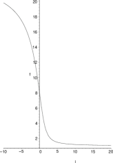
Figure 1: Plot of the function $f$ at the positive and negative regions near the throat. Notice that $f$ is smooth and positive everywhere. The values of the parameters are $l_{0}=2,l_{1}=1,\phi_{0}=1$.

Expanding the gravitational function $f_{\rm st}$ and the scalar field $\phi_{\rm st}$ for large values of the distance coordinate $l$, we have, on the positive side:

$$f_{\rm st} = 1+\frac{\phi_{0}\,\sqrt{l_{0}^{2}-l_{1}^{2}}}{l}+O\left(\frac{1}{l^{2}}\right)$$ (11)

$$\sqrt{\frac{8\pi G}{c^{4}}}\phi_{\rm st} = -\sqrt{2+\frac{\phi_{0}^{2}}{2}}\,\frac{\sqrt{l_{0}^{2}-l_{1}^{2}}}{l}+O\left(\frac{1}{l^{2}}\right)$$ (12)

from where we can read the mass parameter which takes the form $M=-\frac{\phi_{0}\,\sqrt{l_{0}^{2}-l_{1}^{2}}}{2}$ and the scalar field charge $\sqrt{\frac{8\pi G}{c^{4}}}q_{\phi}=-\sqrt{2+\frac{\phi_{0}^{2}}{2}}\,\sqrt{l_{0}^{2}-l_{1}^{2}}$. Notice how the mass parameter depends on the value of $\phi_{0}$ and is positive for negative $\phi_{0}$, the scalar field charge is invariant with respect to the sign of $\phi_{0}$

Now, with respect to the throat, following Morris and Thorne MT , we freeze the time and select the plane angle $\theta=\frac{\pi}{2}$ in that slice obtaining the ${ds_{2}}^{2}=\frac{1}{f}\,\left(dl^{2}+\left(l^{2}-2\,l\,l_{1}+{l_{0}}^{2}\right)\,d\varphi^{2}\right)$. Making the embedding in the cylindrical space $dD^{2}=d\rho^{2}+dz^{2}+\rho^{2}\,d\varphi^{2}$, the shape of the throat is given by $z=z(\rho)$, thus ${dD_{2}}^{2}=\left(1+{z_{,\rho}}^{2}\right)\,d\rho^{2}+\rho^{2}\,d\varphi^{2}$. Comparing the two distant elements we see that $\rho^{2}=\frac{l^{2}-2\,l\,l_{1}+{l_{0}}^{2}}{f}$, and the shape of the throat is given then by $z(\rho)=\int_{\rho_{\rm min}}^{\rho}\,\sqrt{\frac{(l_{,\rho})^{2}}{f(\rho)}-1}\,\,d\rho$. In our case, it turns out to be more convenient to do this procedure in a parametric form, in terms of the distance coordinate $l$, so the value for the throat is given by the pair $\left[\rho(l_{f}),z(l_{f})=\int_{l_{\rm min}}^{l_{f}}\,\sqrt{\frac{1}{f}-(\rho_{,l})^{2}}\,\,dl\right]$. Thus, given an $l_{f}$, we obtain the value of the corresponding pair of coordinates. The integral was solved numerically, the resulting shape of the throat is given in Fig.2. Notice the distinctive shape of the throat.

Figure 2: Shape of the throat for the static WH. The values of the parameters are $l_{0}=3.54,l_{1}=1,\phi_{0}=0.01$. For these values, the minimal length of the throat is $\rho_{\rm min}=3.3692$, for $l_{\rm min}=0.9830$, and we plot for $l_{\rm min}-1$, to $l_{\rm min}+1$.

Solution (5,6,7) includes as particular solution the Ellis-Morris-Thorne one described in terms of the proper distance. This can be seen by taking $\phi_{0}=0,l_{1}=0$, which reduces the static solution to $f=1$ and the scalar field to $\sqrt{\frac{8\pi G}{c^{4}}}\phi=\sqrt{2}\,\left(\lambda-\frac{\pi}{2}\right)$, with $\lambda=\arctan\left(\frac{l}{l_{0}}\right)$, which is just the well known static spherical symmetric solution of Ellis-Morris-Thorne,MT ; Ellis .

In this way, we see that the WH static solution is, by itself, an interesting solution. A deeper study of it, including the geodesic motion of particles, the description of the physical parameters acting on it, as well as a stability analysis, are subjects beyond the aim of the present work, which is to obtain exact solutions to the Einstein-scalar field equations. Thus, we continue to present the case with the rotation parameter $a\neq 0$ for which, as we will show, the field equations can also be solved, describing a rotating wormhole with a deficit angle in the asymptotic regions, and can also be thought to model the region near the throat of a rotating WH. We show that it can be smoothly matched with the asymptotically flat external regions, in particular we match the radial part of it to the static solution presented above.

Figure 3: Plot of the function $f$ for the exterior and interior solutions, observe that for these values the matching of the solutions on the rhs is smooth, while the matching is always smooth on the lhs. The values of the parameters are $l_{1}=0.5,l_{+}=10,\phi_{0}=2,l_{0}=1,a=0.6$ and we plot for radius from -20 to 20.

IV The Rotating Solution

For $a\neq 0$ we find the exact solution:

$$f = 2\,{\frac{{\phi_{0}}\,\sqrt{D\,\left({l_{0}}^{2}-{l_{1}}^{2}\right)}\,{e^{{\phi_{0}}\,\left(\lambda-\frac{\pi}{2}\right)}}}{{a}^{2}+{D}\,{e^{2\,{\phi 0}\,\left(\lambda-\frac{\pi}{2}\right)}}}},$$ (13)

$$\sqrt{\frac{8\pi G}{c^{4}}}\phi = \sqrt{2+\frac{{\phi_{0}}^{2}}{2}}\,\left(\lambda-\frac{\pi}{2}\right),$$ (14)

where the function $\lambda$ is again given by (7), $a$ is the angular momentum parameter and $D$ is an integration constant. It is remarkable that the scalar field has exactly the same expression as in the non-rotating case. Here $\phi_{0}>0$ in order to preserve the signature of the metric. It can be seen that there is a throat, for large values of the distance parameter, $l$, the gravitational functions goes to a constant on both sides, as well as the scalar field, showing that we do have a rotating wormhole solution to the field equations, with a deficit angle. Furthermore, the norm of the Killing-vector $\xi=\frac{\partial}{\partial t}$ is always negative $|\xi|=-f$, thus the solution does not have an ergosphere. As mentioned before, this is the first solution of this type, as long as the other ones known in the literature, rot , only describe the possible geometry of a rotating wormhole, without solving the complete field equations with a specific source of matter.

We can see that indeed the constant $a$ is a rotation parameter by means of the Ernst potential $\mathcal{E}$ (see for example exactsolutions ). Due to the symmetries of the space-time, it is easy to see that the Ernst potential is $\mathcal{E}=f+i\epsilon$, where $\epsilon$ is the rotations potential. For solution (13) the invariant quantity $\epsilon$, is given by

$$\epsilon=-a\frac{\phi_{0}\sqrt{D(l_{0}^{2}-l_{1}^{2})}}{a^{2}+De^{2\phi_{0}(\lambda-\frac{\pi}{2})}},$$ (15)

showing in this way that the parameter $a$ is a parameter of the space-time as claimed.

Even though this is a solution for the complete space-time, we can see it as describing the internal parts of a rotating wormhole, from the throat to some distance on each mouth, and match it with an external, asymptotically flat solution, such as Kerr or the static wormhole presented above. In what follows we present this last matching for the radial part of the solution, showing that it can be a smooth one. Then, the matched function for the rotating WH solution reads

$$f=\left\{\begin{array}[]{cc}\exp(\lambda-\frac{\pi}{2})&\text{if }l>l_{+}\\ &\\ 2\,{\frac{{\phi_{0}}\,\sqrt{D\,\left({l_{0}}^{2}-{l_{1}}^{2}\right)}\,{e^{{\phi_{0}}\,\left(\lambda-\frac{\pi}{2}\right)}}}{{a}^{2}+{D}\,{e^{2\,{\phi_{0}}\,\left(\lambda-\frac{\pi}{2}\right)}}}}&\text{if }l_{-}\leq l\leq l_{+}\\ &\\ \phi_{1}\exp(\lambda+\frac{\pi}{2})&\text{if }l<l_{-}\end{array}\right.$$ (16)

where $l_{-}$ and $l_{+}$ respectively are the matching points on the left and right hand side (see Fig.3). It can be seen that the interior solution matches with the rhs exterior one provided that the parameter $D$ becomes:

$${D} = 2\,{\phi_{0}}\,\sqrt{\left({l_{0}}^{2}-{l_{1}}^{2}\right)\left(\left({l_{0}}^{2}-{l_{1}}^{2}\right){{\phi_{0}}}^{2}-{\frac{{a}^{2}}{{E}^{2}}}\right)}$$ (17)

$$+ 2\,\left({l_{0}}^{2}-{l_{1}}^{2}\right){{\phi_{0}}}^{2}-{\frac{{a}^{2}}{{E}^{2}}}$$

where the constant $E$ is determined by the radio $l_{+}$ where the two solutions match, it is given by:

$$E=\exp\left[{{\phi_{0}}\left(\arctan\left({\frac{{l_{+}-l_{1}}}{\sqrt{l_{0}^{2}-l_{1}^{2}}}}\right)-\frac{\pi}{2}\right)}\right].$$ (18)

In order to have a real solution everywhere we impose the constraint that $4\,M^{2}=\left({l_{0}}^{2}-{l_{1}}^{2}\right){\phi_{0}}^{2}>\frac{{a}^{2}}{{E}^{2}}$. On the other side the matching of the interior solution is smooth with the lhs exterior one, if the constant $\phi_{1}$ is chosen such that

$${\phi_{1}}=2\,{\frac{{\phi_{0}}\,\sqrt{D({l_{0}}^{2}-{l_{1}}^{2})}\,e^{2\,\phi_{0}\,\lambda_{-}}}{{a}^{2}+{D}{e^{2\,{\phi_{0}}\,\left(\lambda_{-}-\frac{\pi}{2}\right)}}}},$$ (19)

where $\lambda_{-}$ is given by Eq. (7), evaluated at $l=l_{-}$. In Fig.3 we see the plot of $f$. Observe that the matching on the rhs could be smooth if $l_{+}$ is sufficiently large and the rotation parameter $a$ is sufficiently small. On the contrary, for small $l_{+}$ or/and big rotation parameter the matching on the rhs is continous but not necessarily smooth. On the lhs and for the scalar field the matching is always smooth. Following the same procedure described above to obtain the shape of the throat, we obtain a similar figure like Fig.2 as for the non-rotating case.

V Physical Aspects of the solution

Let us write the solution in terms of the mass parameter $M$. We start with the constant $D$, it reads

$$D = M^{2}\ \left(4\,\sqrt{4-{\frac{{J}^{2}}{{E}^{2}}}}+8-{\frac{{J}^{2}}{{E}^{2}}}\right)$$ (20)

$$= M^{2}\ d^{2}$$

where $J=a/M$. Observe that $d$ does not depend on the mass parameter $-M=mG/c^{2}$, where $m$ is the total mass of the scalar field star. Furthermore, if we want that the wormhole is transversable, we expect a gravitational field similar to the Earth’s one, this means $m\sim$ Earth’s mass. For this value the mass parameter is $-M\sim 0.01\$ meters. But we want that a spaceship can go trough the throat of the wormhole, we can suppose that $l_{0}\sim 10$ meters, then, $l_{1}\sim 10$ meters as well, depending on the value of $\phi_{0}$. Thus, the interior solution reads

$$f_{int} = 4\,{\frac{-M\,\sqrt{D}\,{e^{{\phi_{0}}\,\left(\lambda-\frac{\pi}{2}\right)}}}{{a}^{2}+{D}\,{e^{2\,{\phi_{0}}\,\left(\lambda-\frac{\pi}{2}\right)}}}}$$ (21)

$$= 4\,{\frac{d\,{e^{{\phi_{0}}\,\left(\lambda-\frac{\pi}{2}\right)}}}{{J}^{2}+d^{2}\,{e^{2\,{\phi_{0}}\,\left(\lambda-\frac{\pi}{2}\right)}}}}$$

where the function $\lambda$ is given by

$$\lambda=\arctan\left(-\phi_{0}\frac{l}{2M}\right)$$ (22)

Observe that $l_{Sch}=-2M$ is the Schwarzschild radius. The scalar field star which provokes the wormhole could be thousands of meters long. Compare with the mass parameter $M$ of orders of millimeters, the matching could be considered as if it were at infinity. In that case the parameter $E=1$. Thus the solution has only 3 parameters, $M,\ J$ and $\phi_{0}$. In this unites $|J|\leq 2$. Then the parameter $d$ is bounded to $2\leq d\leq 4$. Nevertheless, the matching condition on the left hand side (in $l_{-}$) does not depend on the mass parameter $M$, it is given by

$$\phi_{1}=4\,{\frac{d\,{e^{2\,\phi_{0}\,\lambda_{-}}}}{{J}^{2}+d^{2}{e^{2\,\phi_{0}\,\left(\lambda_{-}-\frac{\pi}{2}\right)}}}}.$$ (23)

where $\lambda_{-}=\lambda(l_{-})$. We can take $l_{-}$ such that $\lambda_{-}\simeq-\pi/2$. Thus, on the left hand side the metric at minus infinity can be written as

$$ds^{2}_{\rm far}=-\phi_{1}dt_{+}^{2}+\frac{1}{\phi_{1}}\left(dl_{+}^{2}+l_{+}^{2}d\Omega^{2}\right)=-dt_{-}^{2}+dl_{-}^{2}+l_{-}^{2}d\Omega^{2},$$ (24)

where now $\Delta t_{-}=\sqrt{\phi_{1}}\Delta t_{+}$ and $\Delta l_{-}=\frac{1}{\sqrt{\phi_{1}}}\Delta l_{+}$. The constant $\phi_{1}$ can be very big. Amazingly the major values for $\phi_{1}$ are obtained for small rotation, $J<<1$. It can be seen that $\phi_{1}$ has a maximum value when $\phi_{0}$ is

$$\phi_{0max}=-\frac{1}{2\pi}\ln\left({\frac{{J}^{2}{E}^{2}}{4\,\sqrt{4\,E^{2}-J^{2}}\ E+8\,{E}^{2}-{J}^{2}}}\right)$$ (25)

Thus, an observer on the left hand side space (on $l_{-}$) will feel that the time goes fast for small changes in $\Delta t_{+}$ and will measure small changes of space for big changes on $\Delta l_{+}$. It is left to find a phantom field star with small rotation and scalar charge given by

$$\sqrt{\frac{8\pi G}{c^{4}}}q_{\phi}={2M}\sqrt{\frac{2}{\phi_{0}^{2}}+\frac{1}{2}}$$ (26)

with a scalar charge given by $\phi_{0}=\phi_{0max}$. For example, if the phantom scalar star has a rotation like $J=10^{-10}$, then $\phi_{1}\sim 1.4\times 10^{5}$ when the scalar charge is $q_{\phi}\sim 0.3M\ m_{Plank}$. For a star with an Earth’s mass, this charge is equivalent to $q_{\phi}\sim 0.003\ m_{Plank}$ per meter.

VI Stability of the Solutions

Thus far we have shown that we have indeed solved the field equations and obtained a rotating wormhole, with a static one as a particular case, and presented some physical properties of the solutions. This is the main purpose of the present work. As long as the stability issue is of the most exciting ones, we finish the work with an idea that gives us ground to conjecture that the rotating solution is stable indeed. Of course, the complete analysis, needs a numerical evolution of the perturbed solution, or an analysis of the radiative modes in the Teukolsky equation. Here we present some preliminary results concerning the stability of the solutions. Let $h_{\mu\nu}=h_{\mu\nu}(l,t)<<1$ be a radial perturbation of metric (1), that is

$$ds^{2} = -(f+h_{44})c^{2}\,dt^{2}-2\ a\,\cos\theta\ dt\ d\varphi$$ (27)

$$+ \left(\frac{1}{f}+h_{11}\right)\,dl^{2}+\frac{1}{f}\left(l^{2}+{l_{0}}^{2}\right)\,d\theta^{2}$$

$$+ \left(\frac{1}{f}\left(l^{2}+{l_{0}}^{2}\right)\,\sin^{2}\theta-f\ a\ \cos\theta\right)\,d\varphi^{2},$$

(In this section we make the distance parameter $l_{1}=0$, for simplicity). Now, let us consider a Gaussian ring perturbation in the radial direction centered in $l=L_{0}$, for $\theta=\pi/2$, in such a way that $h_{11}=f_{0}T(t)\exp(-(l-L_{0})^{2}/L_{1})$. Even for this simple perturbation, the field equations are a non-trivial set of differential equations. However, in this case the behavior of the field equations can be reduced to an evolution equation only for $h_{11}$ of the form

$$T_{,tt}+\omega^{2}\ T+\text{terms}$$ (28)

Figure 4: Plot of the function $\omega$ for the Schwarzschild, the Morris-Thorne, the static and the rotating solutions. The Schwarzschild solution has unstable modes only inside the horizon $l=-2M$, but it has stable modes outside, as the rotating solution has. We have set the ring perturbation as $r_{0}=4\ r_{1}=0.1$ and $f_{0}=1\times 10^{-4}$.

where $\omega$ is a function of the radial coordinate $l$ only.

Not pretending to give a demonstration of stability, we can expect that this evolution equation will be oscillating if $\omega^{2}>0$, and monotonic if $\omega^{2}<0$. In Fig.4 we see the results using this criterion for the Schwarzschild, the Morris-Thorne, the static (5) and the rotating (16) solutions. We can interpret these results as follows. We have added a perturbation to the solution in such a way that the Gaussian perturbation simulates the presence of an object in $l=L_{0}$ and remains there. From the curve obtained from the Schwarzschild solution we see that the perturbation provokes monotonic modes for the region $l>L_{0}$, but oscillating modes for the region $l<L_{0}$. Inside the horizon the modes are again monotonic, this does not affect the stability of the object. This might imply that the original object is stable, the perturbed metric oscillates around the original metric for the region inside of the center of the perturbation on $l=L_{0}$. This situation does not happen with the Morris-Thorne solution. There, $\omega=0$ implying that all the modes are monotone everywhere. This can be interpreted as saying that this solution is unstable for these kind of perturbations. In the case of the static solution (5) the modes are monotone for the region $l<L_{0}$, but it is oscillating for the regions $l>L_{0}$. This might imply that the static solution is unstable as well, because the monotonic behavior of the solution close to the center will destroy the object. For the case of the rotating solution (16) the situation is similar as for the Schwarzschild one. The modes in the region $l<L_{0}$ are oscillating, the perturbed solution on this regions only oscillates around the original solution. We see that, according to this criterion, the Schwarzschild solution is stable under this Gaussian perturbation, but the Morris-Thorne and the static are not, and that the rotating solutions is stable. Nevertheless, because this is not a demonstration in general, we leave this result as a conjecture.

If this would be so, then the possible existence of negative kinetic energy scalar fields and its stability could be the door to a new way of travel form through the Universe.

VII Conclusions

We have found a new solution which represents the space-time of a rotating wormhole. This is the first exact solution of the Einstein equations with a scalar field, with negative kinetic term (phantom field), with these features. The solution is matched to an static one which is by self an wormhole solutions with a phantom field source. The solutions present the expected features, they connect to regions of the space-time, where time and space behave in different way in both regions. We found that the different behavior depends on the parameters of the solution, $J,\ M$ and $q_{\phi}$. Slow rotating wormhole stars contain more possibilities to connect a human traveller with more distant regions. We present some calculations of the perturbations which could indicate that the rotating solution is stable under certain perturbations. We consider that counting with an exact solution to the Einstein scalar field equations for a rotating wormhole will certainly contribute to have a better understanding on the physical processes occurring in those regions, suggesting what kind of observations should be made in order to probe the existence or not of wormholes in the Universe.

VIII Acknowledgments

The authors acknowledges Miguel Alcubierre, Olivier Sarbach, Roberto Sussman, Juan Carlos Degollado, Mike Ryan, Abril Suarez and Israel Villagomez for fruitful comments on our work. TM wants to thank Matt Choptuik for his kind hospitality at the UBC. DN is grateful to Vania Jimenez-Lobato for useful discussions to start the elaboration of the present work. This work was partially supported by DGAPA-UNAM grant IN-122002, and CONACyT México, under grants 32138-E and 42748.

References

- (1) A. Einstein, and N. Rosen, Phys. Rev. 48, 73, (1935).
- (2) H. G. Ellis, J. Math. Phys., 14, 395, (1973).
- (3) M. S. Morris, K. S. Thorne, Am. J. of Physics, 56, N. 5, 365, (1988).
- (4) M. Visser, Lorentzian wormholes: form Einstein to Hawking, I. E. P. Press, Woodsbury, N. Y. 1995.
- (5) F. S. N. Lobo, Phys.Rev. D71 (2005) 084011, e-print: gr-qc/0502099.
- (6) T. Roman, e-print: gr-qc/0409090.
- (7) R. Penrose, Battele Rencontres, ed. by B. S. de Witt and J. A. Wheeler, Benjamin, New York, (1968).
- (8) H. Shinkay and S. A. Hayward, Phys. Rev. D , (2002), e-print: gr-qc/0205041.
- (9) E. Teo, e-print: gr-qc/9803098, P. K. F. Kuhfitting, e-print: gr-qc/0401023, e-print: gr-qc/0401028, e-print: gr-qc/0401048.
- (10) Stephani, H., Kramer, D., MacCallum, M., Hoenselaers, C., Herlt, E., Exact soltuions to Einstein’s field equations, 2nd, ed., Cambridge, U. P., U. K., (2003).
- (11) T. Matos, Gen.Rel.Grav.19:481-492,1987. T. Matos, Phys.Rev.D38:3008-3010,1988. T. Matos, Annalen Phys.46:462-472,1989. R. Becerril, T. Matos, Phys.Rev.D41:1895-1896,1990. T. Matos, G. Rodriguez, In *Cocoyoc 1990, Proceedings, Relativity and gravitation: Classical and quantum* 456-462. R.B. Becerril, T.C. Matos, In *Cocoyoc 1990, Proceedings, Relativity and gravitation: Classical and quantum* 504-509. T. Matos, G. Rodriguez, R. Becerril, J.Math.Phys.33:3521-3535,1992. Tonatiuh Matos, J.Math.Phys.35:1302-1321,1994. [GR-QC 9401009]. Tonatiuh Matos, CIEA-GR-94-06 (n.d.) 8p. [HEP-TH 9405082]. Tonatiuh Matos, Dario Nunez, Hernando Quevedo, Phys.Rev.D51:310-313,1995. [GR-QC 9510042]. Tonatiuh Matos, Cesar Mora, Class.Quant.Grav.14:2331-2340,1997. [HEP-TH 9610013]. Tonatiuh Matos, Cesar Mora, Class.Quant.Grav.14:2331-2340,1997. [HEP-TH 9610013]. Tonatiuh Matos, Phys.Lett.A249:271-274,1998. [GR-QC 9810034]. T. Matos, U. Nucamendi, P. Wiederhold, J.Math.Phys.40:2500-2513,1999. T. Matos, M. Rios, Gen.Rel.Grav.31:693-700,1999. Tonatiuh Matos, Dario Nunez, Gabino Estevez, Maribel Rios, Gen.Rel.Grav.32:1499-1525,2000. [GR-QC 0001039]. Tonatiuh Matos, Dario Nunez, Maribel Rios, Class.Quant.Grav.17:3917-3934,2000. [GR-QC 0008068].
- (12) Jian-gang Hao, Xin-zhou Li.Phys.Rev. D67 (2003) 107303. L.P. Chimento, Ruth Lazkoz. Phys.Rev.Lett. 91 (2003) 211301. German Izquierdo, Diego Pavon. astro-ph/0505601. S. V. Sushkov.Phys.Rev. D71 (2005) 043520.
- (13) D. Kramer, H. Stephani, M. MacCallum and E. Herlt. Exact Solutions of Einstein Field Equations. VEB Deutscher Verlag der Wissenschaften, Berlin, 1980.