Stable dark energy stars

Abstract

The gravastar picture is an alternative model to the concept of a black hole, where there is an effective phase transition at or near where the event horizon is expected to form, and the interior is replaced by a de Sitter condensate. In this work, a generalization of the gravastar picture is explored, by considering a matching of an interior solution governed by the dark energy equation of state, $\omega\equiv p/\rho<-1/3$, to an exterior Schwarzschild vacuum solution at a junction interface. The motivation for implementing this generalization arises from the fact that recent observations have confirmed an accelerated cosmic expansion, for which dark energy is a possible candidate. Several relativistic dark energy stellar configurations are analyzed by imposing specific choices for the mass function. The first case considered is that of a constant energy density, and the second choice, that of a monotonic decreasing energy density in the star’s interior. The dynamical stability of the transition layer of these dark energy stars to linearized spherically symmetric radial perturbations about static equilibrium solutions is also explored. It is found that large stability regions exist that are sufficiently close to where the event horizon is expected to form, so that it would be difficult to distinguish the exterior geometry of the dark energy stars, analyzed in this work, from an astrophysical black hole.

I Introduction

The structure of relativistic stars and the phenomenon of gravitational collapse is of fundamental importance in astrophysics and has attracted much attention in the relativist community since the formulation of general relativity. Relatively to the construction of theoretical models of relativistic stars, one may refer to the pioneering work of Schwarzschild Schw , Tolman Tolman , and Oppenheimer and Volkoff OppVolk . Schwarzschild Schw considered analytic solutions describing a star of uniform density, and Tolman Tolman developed a method providing explicit solutions for static spheres of fluid, which proved important to the study of stellar structure. Oppenheimer and Volkoff OppVolk by suitably choosing specific Tolman solutions studied the gravitational equilibrium of neutron stars, using the equation of state for a cold Fermi gas, consequently laying down the foundations of the general relativistic theory of stellar structures. Paging through history one finds an extremely extensive literature Gravitation , however, one may refer to the important contributions of Chandrasekhar Chand in the construction of white-dwarf models by taking into account special relativistic effects in the electron degeneracy equation of state, where he discovered that no white dwarf may have a mass greater than $\sim 1.2$ solar masses, which has been called the Chandrasekhar limit; and the work of Baade and Zwicky neutron , where they invented the concept of a neutron star, and identified astronomical objects denoted as supernovae, representing a transitional collapse of an ordinary star into a neutron star. Far from undertaking an exhaustive review, one may also refer to the work of Wyman, where in Ref. Wyman1 isotropic coordinates were used to solve the relativistic equations of a perfect fluid with constant energy density, and in Ref. Wyman2 , a critical examination and generalization of the Tolman solutions was undertaken; Buchdahl Buchdahl and Bondi Bondi generalized the interior Schwarzschild solution to more general static fluid spheres in the form of inequalities involving the mass concentration, central energy density and central pressure; Leibovitz Leib also generalized some of Tolman’s solutions by applying a more physical approach; and the discovery of pulsars by Hewish et al Hewish , the idea advanced by Gold Gold that pulsars might be rotating neutron stars, which was later confirmed by observations, and the idealized models of rotating neutron stars rotate-neutron . It is also interesting to note that Bayin found new solutions for static fluid spheres Bayin1 , explored the time-dependent field equations for radiating fluid spheres Bayin2 , and further generalized the analysis to anisotropic fluid spheres Bayin3 .

Relatively to the issue of gravitational collapse, before the mid-1960s, the object now known as a black hole, was referred to as a collapsed star Thorne-etal . Oppenheimer and Snyder OppSnyd , in 1939, provided the first insights of the gravitational collapse into a black hole, however, it was only in 1965 that marked an era of intensive research into black hole physics. Although evidence for the existence of black holes is very convincing, it has recently been argued that the observational data can provide very strong arguments in favor of the existence of event horizons but cannot fundamentally prove it AKL . This scepticism has inspired new and fascinating ideas. In this line of thought, it is interesting to note that a new final state of gravitational collapse has been proposed by Mazur and Mottola Mazur . In this model, and in the related picture developed by Laughlin et al Laughlin , the quantum vacuum undergoes a phase transition at or near the location where the event horizon is expected to form. The model denoted as a gravastar (gravitational vacuum star), consists of a compact object with an interior de Sitter condensate, governed by an equation of state given by $p=-\rho$, matched to a shell of finite thickness with an equation of state $p=\rho$. The latter is then matched to an exterior Schwarzschild vacuum solution. The thick shell replaces both the de Sitter and the Schwarzschild horizons, therefore, this gravastar model has no singularity at the origin and no event horizon, as its rigid surface is located at a radius slightly greater than the Schwarzschild radius. It has been argued that there is no way of distinguishing a Schwarzschild black hole from a gravastar from observational data AKL . It was also further shown by Mazur and Mottola that gravastars are thermodynamically stable. Related models, analyzed in a different context have also been considered by Dymnikova Dymnikova . However, in a simplified model of the Mazur-Mottola picture, Visser and Wiltshire VW constructed a model by matching an interior solution with $p=-\rho$ to an exterior Schwarzschild solution at a junction interface, comprising of a thin shell. The dynamic stability was then analyzed, and it was found that some physically reasonable stable equations of state for the transition layer exist. In Ref. CFV , a generalized class of similar gravastar models that exhibit a continuous pressure profile, without the presence of thin shells was analyzed. It was found that the presence of anisotropic pressures are unavoidable, and the TOV equation was used to place constraints on the anisotropic parameter. It was also found that the transverse pressures permit a higher compactness than is given by the Buchdahl-Bondi bound Buchdahl ; Bondi for perfect fluid stars, and several features of the anisotropic equation of state were explored. In Ref. Bilic , motivated by low energy string theory, an alternative model was constructed by replacing the de Sitter regime with an interior solution governed by a Chaplygin gas equation of state, interpreted as a Born-Infeld phantom gravastar.

It has also been recently proposed by Chapline that this new emerging picture consisting of a compact object resembling ordinary spacetime, in which the vacuum energy is much larger than the cosmological vacuum energy, has been denoted as a “dark energy star” Chapline . In fact, in the present paper a mathematical model generalizing the Mazur-Mottola picture, or for that matter, the Visser-Wiltshire model is proposed, where the interior de Sitter solution is replaced by a solution governed by the dark energy equation of state, $p=\omega\rho$ with $\omega<-1/3$, matched to an exterior vacuum Schwarzschild solution. Note that the particular case of $\omega=-1$ reduces to the Visser-Wiltshire gravastar model. The motivation for implementing this generalization comes from the fact that recent observations have confirmed that the Universe is undergoing a phase of accelerated expansion. Evidence of this cosmological expansion has been shown independently from measurements of supernovae of type Ia (SNe Ia) supernovae and from cosmic microwave background radiation CMB . A possible candidate proposed for this cosmic acceleration is precisely that of dark energy, a cosmic fluid parametrized by an equation of state $\omega\equiv p/\rho<-1/3$, where $p$ is the spatially homogeneous pressure and $\rho$ the dark energy density. If $\omega<-1$, a case certainly not excluded, and in fact favored, by observations, the null energy condition is violated. For this case, the cosmic fluid is denoted phantom energy, and possesses peculiar properties, such as negative temperatures dark-entropy and the energy density increases to infinity in a finite time, resulting in a Big Rip Weinberg . It also provides one with a natural scenario for the existence of exotic geometries such as wormholes Sushkov ; Lobo-phantom . In this context, it was also shown that the masses of all black holes tend to zero as the phantom energy universe approaches the Big Rip Babichev . However, it is interesting that recent fits to supernovae, CMB and weak gravitational lensing data favor an equation of state with a dark energy parameter crossing the phantom divide $\omega=-1$ Vikman ; phantom-divide . In a cosmological setting the transition into the phantom regime, for a single scalar field Vikman is probably physically implausible, thus the stress energy tensor should include a mixture of various interacting non-ideal fluids.

As emphasized in Refs. Sushkov ; Lobo-phantom , in a rather different context, a subtlety needs to be pointed out: The notion of dark energy is that of a spatially homogeneous cosmic fluid, however, it can be extended to inhomogeneous spherically symmetric spacetimes by regarding that the pressure in the dark energy equation of state is a negative radial pressure, and the transverse pressure may be determined via the field equations. (An inhomogeneous spherically symmetric dark energy scalar field was also considered in Ref. Picon-Lim ). In this context, the generalization of the gravastar picture with the inclusion of an interior solution governed by the equation of state, $p=\omega\rho$ with $\omega<-1/3$, will be denoted by a dark energy gravastar, or simply a “dark energy star” in agreement with the Chapline definition Chapline . We shall explore several configurations, by imposing specific choices for the mass function. We shall then explore the dynamical stability of the transition layer of these models to linearized perturbations around static solutions, by applying the general stability formalism developed in Ref. LoboCrawford , and which was also applied in the context of the stability of phantom wormholes stableWH , and further analyze the evolution identity to extract some physical insight regarding the pressure balance equation across the junction interface. The dark energy star outlined in this paper may possibly have an origin in a density fluctuation in the cosmological background. It is uncertain how such inhomogeneities in the dark energy may be formed. However, a possible explanation may be inferred from Ref. inhomogEOS , where the dark energy equation of state was generalized to include an inhomogeneous Hubble parameter dependent term, possibly resulting in the nucleation of a dark energy star through a density perturbation.

This paper is outlined in the following manner. In Section II, we present the structure equations of dark energy stellar models. In Section III, specific models are then analyzed by imposing particular choices for the mass function. In Section IV, the linearized stability analysis procedure is briefly outlined, and the stability regions of the transition layer of specific dark energy stars are determined. Finally in Section V, we conclude.

II Dark energy stars: Equations of structure

Consider the interior spacetime, without a loss of generality, given by the following metric, in curvature coordinates

$$ds^{2} = -{\rm exp}\left[-2\int_{r}^{\infty}g(\tilde{r})d\tilde{r}\right]\,dt^{2}+\frac{dr^{2}}{1-2m(r)/r}$$ (1)

$$+r^{2}\,(d\theta^{2}+\sin^{2}{\theta}\,d\phi^{2})\,,$$

where $g(r)$ and $m(r)$ are arbitrary functions of the radial coordinate, $r$. The function $m(r)$ is the quasi-local mass, and is denoted as the mass function. The factor $g(r)$ is the “gravity profile” and is related to the locally measured acceleration due to gravity, through the following relationship: ${\cal A}=\sqrt{1-2m(r)/r}\,g(r)$ Martin ; Martin2 . The convention used is that $g(r)$ is positive for an inwardly gravitational attraction, and negative for an outward gravitational repulsion. Note that equivalently one may consider a function $\Phi(r)$, defined as $\Phi(r)=-\int_{r}^{\infty}g(\tilde{r})d\tilde{r}$, and denoted as the redshift function, as it is related to the gravitational redshift Morris .

The stress-energy tensor for an anisotropic distribution of matter is provided by

$$T_{\mu\nu}=(\rho+p_{t})U_{\mu}\,U_{\nu}+p_{t}\,g_{\mu\nu}+(p_{r}-p_{t})\chi_{\mu}\chi_{\nu}\,,$$ (2)

where $U^{\mu}$ is the four-velocity, $\chi^{\mu}$ is the unit spacelike vector in the radial direction, i.e., $\chi^{\mu}=\sqrt{1-2m/r}\,\delta^{\mu}{}_{r}$. $\rho(r)$ is the energy density, $p_{r}(r)$ is the radial pressure measured in the direction of $\chi^{\mu}$, and $p_{t}(r)$ is the transverse pressure measured in the orthogonal direction to $\chi^{\mu}$.

Thus, the Einstein field equation, $G_{\mu\nu}=8\pi T_{\mu\nu}$, where $G_{\mu\nu}$ is the Einstein tensor, provides the following relationships

$$m^{\prime} = 4\pi r^{2}\rho\,,$$ (3)

$$g = \frac{m+4\pi r^{3}p_{r}}{r(r-2m)}\,,$$ (4)

$$p_{r}^{\prime} = -\frac{(\rho+p_{r})(m+4\pi r^{3}p_{r})}{r(r-2m)}+\frac{2}{r}(p_{t}-p_{r})\,.,$$ (5)

where the prime denotes a derivative with respect to the radial coordinate, $r$. Equation (5) corresponds to the anisotropic pressure Tolman-Oppenheimer-Volkoff (TOV) equation.

Now, using the dark energy equation of state, $p_{r}=\omega\rho$, and taking into account Eqs. (3) and (4), we have the following relationship

$$g(r)=\frac{m+\omega rm^{\prime}}{r\,\left(r-2m\right)}\,.$$ (6)

There is, however, a subtle point that needs to be emphasized Sushkov ; Lobo-phantom . The notion of dark energy is that of a spatially homogeneous cosmic fluid. Nevertheless, it can be extended to inhomogeneous spherically symmetric spacetimes, by regarding that the pressure in the equation of state $p=\omega\rho$ is a radial pressure, and that the transverse pressure may be obtained from Eq. (5). Note that for the particular case of $\omega=-1$, from Eq. (6), one has the following solution $g_{tt}=-(1-2m/r)$, which reduces to the specific class of solutions analyzed in Ref. VW .

Using the dark energy equation of state $p_{r}=\omega\rho$, Eq. (5) in terms of the principal pressures, takes the form

$$p_{r}^{\prime}=-p_{r}\left(\frac{1+\omega}{\omega}\right)\,\frac{m+\omega rm^{\prime}}{r\,\left(r-2m\right)}+\frac{2}{r}\,(p_{t}-p_{r})\,,$$ (7)

which taking into account Eq. (3), may be expressed in the following equivalent form

$$\Delta=\frac{\omega}{8\pi r^{2}}\left[m^{\prime\prime}r-2m^{\prime}+\left(\frac{1+\omega}{\omega}\right)m^{\prime}rg\right]\,.$$ (8)

$\Delta=p_{t}-p_{r}$ is denoted as the anisotropy factor, as it is a measure of the pressure anisotropy of the fluid comprising the dark energy star. $\Delta=0$ corresponds to the particular case of an isotropic pressure dark energy star. Note that $\Delta/r$ represents a force due to the anisotropic nature of the stellar model, which is repulsive, i.e., being outward directed if $p_{t}>p_{r}$, and attractive if $p_{t}<p_{r}$.

One now has at hand four equations, namely, the field equations (3)-(5) and Eq. (6), with five unknown functions of $r$, i.e., $\rho(r)$, $p_{r}(r)$, $p_{t}(r)$, $g(r)$ and $m(r)$. Obtaining explicit solutions to the Einstein field equations is extremely difficult due to the nonlinearity of the equations, although the problem is mathematically well-defined. However, in the spirit of Ref. Lobo-phantom , we shall adopt the approach in which a specific choice for a physically reasonable mass function $m(r)$ is provided and through Eq. (6), $g(r)$ is determined, thus consequently providing explicit expressions for the stress-energy tensor components. In the specific cases that follow, we shall consider that the energy density be positive and finite at all points in the interior of the dark energy star.

III Specific models

III.1 Constant energy density

Consider the specific case of a constant energy density, $\rho(r)=\rho_{0}$, so that Eq. (3) provides the following mass function

$$m(r)=\frac{4\pi\rho_{0}}{3}r^{3}\,.$$ (9)

Thus, using Eq. (6), one finds that $g(r)$ is given by

$$g(r)=\frac{Ar(1+3\omega)}{1-2Ar^{2}}\,,$$ (10)

where for simplicity, the definition $A=4\pi\rho_{0}/3$ is used. Note that for $\omega<-1/3$, we have an outward gravitational repulsion, $g(r)<0$, which is to be expected in gravastar models.

The spacetime metric for this solution takes the following form

$$ds^{2} = -\left(1-2Ar^{2}\right)^{-(1+3\omega)/2}\,dt^{2}+\frac{dr^{2}}{1-2Ar^{2}}$$ (11)

$$+r^{2}\,(d\theta^{2}+\sin^{2}{\theta}\,d\phi^{2})\,.$$

The stress-energy tensor components are given by $p_{r}=\omega\rho_{0}$ and

$$p_{t}=\omega\rho_{0}\left[1+\frac{(1+\omega)(1+3\omega)Ar^{2}}{2\omega(1-2Ar^{2})}\right]\,.$$ (12)

The anisotropy factor is provided by

$$\Delta=\frac{3}{8\pi}(1+\omega)(1+3\omega)\frac{A^{2}r^{2}}{1-2Ar^{2}}\,.$$ (13)

One readily verifies that $\Delta<0$ for $-1<\omega<-1/3$ and $\Delta>0$ in the phantom regime, $\omega<-1$. However, it is perhaps instructive to plot $\Delta$, which is depicted in Fig. 1. Note that $\Delta=0$ at the origin, $r=0$, as was to be expected. For $\omega=-1$, then $\Delta=0$ is also verified for arbitrary $r$. This latter condition is also readily derived from Eq. (5), where taking into account $p_{r}=\omega\rho$ for $p_{r}={\rm const}$, one verifies $p_{t}=p_{r}$.

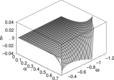
Figure 1: Plot of the anisotropy factor for a dark energy star with a constant energy density. We have defined the following dimensionless parameters: $\delta=\Delta/A$ and $\alpha=\sqrt{A}r$. We verify that $\Delta<0$ in the range $-1/3>\omega>-1$ and $\Delta>0$ in the phantom regime, $\omega<-1$.

III.2 Tolman-Matese-Whitman mass function

Consider the following choice for the mass function, given by

$$m(r)=\frac{b_{0}r^{3}}{2(1+2b_{0}r^{2})}\,,$$ (14)

where $b_{0}$ is a non-negative constant. The latter may be determined from the regularity conditions and the finite character of the energy density at the origin $r=0$, and is given by $b_{0}=8\pi\rho_{c}/3$, where $\rho_{c}$ is the energy density at $r=0$.

This choice of the mass function represents a monotonic decreasing energy density in the star interior, and was used previously in the analysis of isotropic fluid spheres by Matese and Whitman MatWhit as a specific case of the Tolman type$-IV$ solution Tolman , and later by Finch and Skea Finch . Anisotropic stellar models, with the respective astrophysical applications, were also extensively analyzed in Refs. Mak , by considering a specific case of the Matese-Whitman mass function. The numerical results outlined show that the basic physical parameters, such as the mass and radius, of the model can describe realistic astrophysical objects such as neutron stars Mak .

Using Eq. (6), $g(r)$ is given by

$$g(r)=\left(\frac{b_{0}r}{2}\right)\left[\frac{(1+3\omega)+(1+\omega)2b_{0}r^{2}}{(1+b_{0}r^{2})(1+2b_{0}r^{2})}\right]\,,$$ (15)

which is plotted in Fig. 2. Note that $g(r)>0$, for $\omega>-(1+2b_{0}r^{2})/(3+2b_{0}r^{2})$, indicating an inwardly gravitational attraction; from the plot one verifies that, qualitatively, $g(r)$ is positive for values of $\omega$ in the neighborhood of $-1/3$. Now, to be a solution of a gravastar, it is necessary that the local acceleration due to gravity of the interior solution be repulsive, so that the region above-mentioned for which $g(r)>0$ is necessarily excluded.

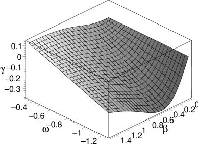
Figure 2: Plot of the “gravity profile” for the Tolman-Matese-Whitman mass function. We have defined the following dimensionless parameters: $\gamma=g(r)/\sqrt{b_{0}}$ and $\beta=\sqrt{b_{0}}r$. Note that, qualitatively, $g(r)$ takes positive values of $\omega$ in the neighborhood of $-1/3$, indicating an inwardly gravitational attraction. To be a solution of a gravastar, it is necessary that the local acceleration due to gravity of the interior solution be repulsive, so that the region for which $g(r)>0$ is necessarily excluded. See the text for details.

The spacetime metric for this solution is provided by

$$ds^{2} = -\left(1+b_{0}r^{2}\right)^{(1-\omega)/2}\left(1+2b_{0}r^{2}\right)^{\omega}\,dt^{2}$$ (16)

$$+\left(\frac{1+2b_{0}r^{2}}{1+b_{0}r^{2}}\right)dr^{2}+r^{2}\,(d\theta^{2}+\sin^{2}{\theta}\,d\phi^{2})\,.$$

The stress-energy tensor components are given by

$$p_{r} = \omega\rho=\left(\frac{\omega b_{0}}{8\pi}\right)\left[\frac{3+2b_{0}r^{2}}{(1+2b_{0}r^{2})^{2}}\right]$$

$$p_{t} = -\left(\frac{b_{0}}{8\pi}\right)\left[\frac{\omega(3+2b_{0}r^{2})}{(1+2b_{0}r^{2})^{2}}\right]+\left(\frac{b_{0}^{2}r^{2}}{32\pi}\right)\times$$ (17)

$$\times\Big{\{}(1+\omega)(3+2b_{0}r^{2})\left[(1+3\omega)+2b_{0}r^{2}(1+\omega)\right]$$

$$-8\omega(5+2b_{0}r^{2})(1+b_{0}r^{2})\Big{\}}\big{/}\left[(1+2b_{0}r^{2})^{3}(1+b_{0}r^{2})\right].$$

The anisotropy factor takes the following form

$$\Delta = \frac{b_{0}^{2}r^{2}}{32\pi}\Big{\{}(1+\omega)(3+2b_{0}r^{2})\left[(1+3\omega)+2b_{0}r^{2}(1+\omega)\right]$$ (18)

$$-8\omega(5+2b_{0}r^{2})(1+b_{0}r^{2})\Big{\}}\big{/}\left[(1+2b_{0}r^{2})^{3}(1+b_{0}r^{2})\right],$$

which is plotted in Fig. 3, where one verifies $\Delta>0$. For the particular case of $\omega=-1$, the anisotropy factor reduces to

$$\Delta=\left(\frac{b_{0}^{2}r^{2}}{4\pi}\right)\frac{(5+2b_{0}r^{2})}{(1+2b_{0}r^{2})^{3}}\,.$$ (19)

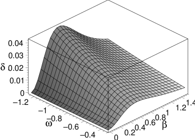
Figure 3: Plot of the anisotropy factor for the Tolman-Matese-Whitman mass function. We have defined the following dimensionless parameters: $\delta=\Delta/b_{0}$ and $\beta=\sqrt{b_{0}}r$. Note that $\Delta>0$ for generic $\omega$ and $r$.

IV Stability of dark energy stars

IV.1 Junction conditions

In this article, we shall model dark energy stars by matching an interior solution, governed by an equation of state, $p=\omega\rho$ with $\omega<-1/3$, to an exterior Schwarzschild vacuum solution with $p=\rho=0$, at a junction interface $\Sigma$, with junction radius $a$. The Schwarzschild metric is given by

$$ds^{2}=-\left(1-\frac{2M}{r}\right)\,dt^{2}+\frac{dr^{2}}{1-\frac{2M}{r}}+r^{2}\,(d\theta^{2}+\sin^{2}{\theta}\,d\phi^{2})\,,$$ (20)

which possesses an event horizon at $r_{b}=2M$. To avoid the latter, the junction radius lies outside $2M$, i.e., $a>2M$. We shall show below that $M$, in this context, may be interpreted as the total mass of the dark energy star. (In an analogous manner traversable wormhole models were constructed in Refs. wormhole-Lobo and the stability analysis of phantom wormholes was carried out in Ref. stableWH .) One may also impose boundary and regularity conditions, and their respective constraints Martin ; bound-constraints , at the center and at the surface of the dark energy star, without the presence of thin shells, however, this analysis will be presented in a subsequent paper.

Using the Darmois-Israel formalism Darmois-Israel , the surface stress-energy tensor $S^{i}_{j}$ at the junction surface $\Sigma$ is given by the Lanczos equations, $S^{i}_{j}=-\frac{1}{8\pi}(\kappa^{i}_{j}-\delta^{i}_{j}\kappa^{k}_{k})$. $\kappa^{i}_{j}$ is defined by the discontinuity of the extrinsic curvatures, $K^{i}_{j}$, across the junction interface, i.e., $\kappa_{ij}=K^{+}_{ij}-K^{-}_{ij}$. The extrinsic curvature is defined as $K_{ij}=n_{\mu;\nu}\,e^{\mu}_{(i)}e^{\nu}_{(j)}$, where $n^{\mu}$ is the unit normal $4-$vector to $\Sigma$, and $e^{\mu}_{(i)}$ are the components of the holonomic basis vectors tangent to $\Sigma$. Using the metrics (1) and (20), the non-trivial components of the extrinsic curvature are given by (see Ref. LoboCrawford for further details)

$$K^{\tau\;+}_{\;\;\tau} = \frac{\frac{M}{a^{2}}+\ddot{a}}{\sqrt{1-\frac{2M}{a}+\dot{a}^{2}}}\;,$$ (21)

$$K^{\tau\;-}_{\;\;\tau} = \frac{\frac{m+\omega am^{\prime}}{a^{2}}+\ddot{a}-\frac{(1+\omega)m^{\prime}\dot{a}^{2}}{(a-2m)}}{\sqrt{1-\frac{2m(a)}{a}+\dot{a}^{2}}}\;,$$ (22)

and

$$K^{\theta\;+}_{\;\;\theta} = \frac{1}{a}\sqrt{1-\frac{2M}{a}+\dot{a}^{2}}\;,$$ (23)

$$K^{\theta\;-}_{\;\;\theta} = \frac{1}{a}\sqrt{1-\frac{2m(a)}{a}+\dot{a}^{2}}\;,$$ (24)

where the overdot denotes a derivative with respect to the proper time, $\tau$, and the prime henceforth shall denote a derivative with respect to $a$. Equation (6) evaluated at $a$ has been used to eliminate $g(r)$ from Eq. (22). In the analysis that follows, we shall apply the same procedure, so that in deducing the master equation, which dictates the stability regions, one shall only make use of the mass function $m(r)$. Thus, the Lanczos equations provide the surface stresses given by

$$\sigma = -\frac{1}{4\pi a}\left(\sqrt{1-\frac{2M}{a}+\dot{a}^{2}}-\sqrt{1-\frac{2m}{a}+\dot{a}^{2}}\,\right),$$ (25)

$${\cal P} = \frac{1}{8\pi a}\Bigg{(}\frac{1-\frac{M}{a}+\dot{a}^{2}+a\ddot{a}}{\sqrt{1-\frac{2M}{a}+\dot{a}^{2}}}$$ (26)

$$-\frac{1+\omega m^{\prime}-\frac{m}{a}+\dot{a}^{2}+a\ddot{a}+\frac{\dot{a}^{2}m^{\prime}(1+\omega)}{1-2m/a}}{\sqrt{1-\frac{2m}{a}+\dot{a}^{2}}}\,\Bigg{)}\,,$$

$\sigma$ and ${\cal P}$ are the surface energy density and the tangential surface pressure, respectively.

We shall also use the conservation identity given by $S^{i}_{j|i}=\left[T_{\mu\nu}e^{\mu}_{(j)}n^{\nu}\right]^{+}_{-}$, where $[X]^{+}_{-}$ denotes the discontinuity across the surface interface, i.e., $[X]^{+}_{-}=X^{+}|_{\Sigma}-X^{-}|_{\Sigma}$. The momentum flux term in the right hand side corresponds to the net discontinuity in the momentum flux $F_{\mu}=T_{\mu\nu}\,U^{\nu}$ which impinges on the shell. The conservation identity is a statement that all energy and momentum that plunges into the thin shell, gets caught by the latter and converts into conserved energy and momentum of the surface stresses of the junction.

Note that $S^{i}_{\tau|i}=-\left[\dot{\sigma}+2\dot{a}(\sigma+{\cal P})/a\right]$, and the flux term is given by (see Ref. LoboCrawford for details)

$$\left[T_{\mu\nu}e^{\mu}_{(j)}n^{\nu}\right]^{+}_{-}=-\frac{(\rho+p_{r})\dot{a}\sqrt{1-2m/a+\dot{a}^{2}}}{1-2m/a}\,,$$ (27)

where $\rho$ and $p_{r}$ may be deduced from Eqs. (3)-(4), respectively, evaluated at the junction radius, $a$. Therefore, using these relationships, the conservation identity provides us with

$$\sigma^{\prime}=-\frac{2}{a}\,(\sigma+{\cal P})+\Xi\,,$$ (28)

where $\Xi$, defined for notational convenience, is given by

$$\Xi=-\frac{1}{4\pi a}\frac{m^{\prime}(1+\omega)}{\left(a-2m\right)}\sqrt{1-\frac{2m}{a}+\dot{a}^{2}}\,,$$ (29)

using Eq. (6) evaluated at $a$. Note that the flux term is zero when $\omega=-1$, which reduces to the analysis considered in Ref. VW .

Taking into account Eqs. (25)-(26) and Eq. (29), then Eq. (28) finally takes the form

$$\sigma^{\prime} = \frac{1}{4\pi a^{2}}\Bigg{(}\frac{1-\frac{3M}{a}+\dot{a}^{2}-a\ddot{a}}{\sqrt{1-\frac{2M}{a}+\dot{a}^{2}}}$$ (30)

$$-\frac{1-\frac{3m}{a}+m^{\prime}+\dot{a}^{2}-a\ddot{a}}{\sqrt{1-\frac{2m}{a}+\dot{a}^{2}}}\,\Bigg{)}\,,$$

which evaluated at a static solution, $a_{0}$, shall play a fundamental role in determining the stability regions. (A linearized stability analysis of spherically symmetric thin shells and of thin-shell wormholes where the flux term is zero was studied in Refs. linear-WH ).

The surface mass of the thin shell is given $m_{s}=4\pi a^{2}\sigma$. By rearranging Eq. (25), evaluated at a static solution $a_{0}$, one obtains the total mass of the dark energy star, given by

$$M=m(a_{0})+m_{s}(a_{0})\left[\sqrt{1-\frac{2m(a_{0})}{a_{0}}}-\frac{m_{s}(a_{0})}{2a_{0}}\right]\,.$$ (31)

Using $m_{s}=4\pi a^{2}\sigma$, and taking into account the radial derivative of $\sigma^{\prime}$, Eq. (28) can be rearranged to provide the following relationship

$$\left(\frac{m_{s}}{2a}\right)^{\prime\prime}=\Upsilon-4\pi\sigma^{\prime}\eta\,,$$ (32)

with the parameter $\eta$ defined as $\eta={\cal P}^{\prime}/\sigma^{\prime}$, and $\Upsilon$ given by

$$\Upsilon\equiv\frac{4\pi}{a}\,(\sigma+{\cal P})+2\pi a\,\Xi^{\prime}\,.$$ (33)

Equation (32) will play a fundamental role in determining the stability regions of the respective solutions. $\eta$ is used as a parametrization of the stable equilibrium, so that there is no need to specify a surface equation of state. The parameter $\sqrt{\eta}$ is normally interpreted as the speed of sound, so that one would expect that $0<\eta\leq 1$, based on the requirement that the speed of sound should not exceed the speed of light. We refer the reader to Refs. linear-WH for discussions on the respective physical interpretation of $\eta$ in the presence of exotic matter.

It is also of interest to analyze the evolution identity, given by: $\left[\,T_{\mu\nu}\,n^{\mu}n^{\nu}\right]^{+}_{-}=\overline{K}^{i}_{\;\,j}\,S^{j}_{\;\,i}$, where $\overline{K}^{i}_{\;\,j}=(K^{i\;+}_{\;\,j}+K^{i\;-}_{\;\,j})/2$. The evolution identity provides the following relationship

$$p_{r}+\frac{(\rho+p_{r})\dot{a}^{2}}{1-2m/a}=-\frac{1}{a}\,\Bigg{(}\sqrt{1-\frac{2M}{a}+\dot{a}^{2}}$$

$$+\sqrt{1-\frac{2m}{a}+\dot{a}^{2}}\;\Bigg{)}\,{\cal P}+\frac{1}{2}\Bigg{(}\frac{M/a^{2}+\ddot{a}}{\sqrt{1-\frac{2M}{a}+\dot{a}^{2}}}$$

$$+\frac{m+\omega am^{\prime}+\ddot{a}a^{2}+\frac{(1+\omega)am^{\prime}\dot{a}^{2}}{1-2m/a}}{a^{2}\sqrt{1-\frac{2m}{a}+\dot{a}^{2}}}\Bigg{)}\sigma\,.$$ (34)

It is of particular interest to obtain an equation governing the behavior of the radial pressure in terms of the surface stresses at the junction boundary, at the static solution $a_{0}$, with $\dot{a}=\ddot{a}=0$. From Eq. (IV.1), we have the following pressure balance equation

$$p_{r}(a_{0}) = -\frac{1}{a_{0}}\,\left(\sqrt{1-\frac{2M}{a_{0}}}+\sqrt{1-\frac{2m}{a_{0}}}\;\right)\,{\cal P}$$ (35)

$$+\frac{1}{2a_{0}^{2}}\left(\frac{M}{\sqrt{1-\frac{2M}{a_{0}}}}+\frac{m+\omega a_{0}m^{\prime}}{\sqrt{1-\frac{2m}{a_{0}}}}\right)\sigma\,.$$

Equation (35) relates the interior radial pressure impinging on the shell in terms of a combination of the surface stresses, $\sigma$ and ${\cal P}$, given by eqs. (25)-(26) evaluated at the static solution, and the geometrical quantities. To gain some insight into the analysis, consider a zero surface energy density, $\sigma=0$. Thus, Eq. (35) reduces to

$$p_{r}(a_{0})=-\frac{2}{a_{0}}\,\sqrt{1-\frac{2M}{a_{0}}}\;\,{\cal P}\,.$$ (36)

As the pressure acting on the shell from the interior is negative $p_{r}(a_{0})<0$, i.e., a radial tension, then a positive tangential surface pressure, ${\cal P}>0$, is needed to hold the thin shell against collapse.

IV.2 Derivation of the master equation

Equation (25) may be rearranged to provide the thin shell’s equation of motion, i.e., $\dot{a}^{2}+V(a)=0$, with the potential given by

$$V(a)=F(a)-\left[\frac{m_{s}(a)}{2a}\right]^{2}-\left[\frac{aG(a)}{m_{s}(a)}\right]^{2}\,.$$ (37)

where, for notational convenience, the factors $F(a)$ and $G(a)$ are defined as

$$F(a)=1-\frac{m(a)+M}{a}\quad{\rm and}\quad G(a)=\frac{M-m(a)}{a}\,.$$ (38)

Linearizing around a stable solution situated at $a_{0}$, we consider a Taylor expansion of $V(a)$ around $a_{0}$ to second order, given by

$$V(a) = V(a_{0})+V^{\prime}(a_{0})(a-a_{0})$$ (39)

$$+\frac{1}{2}V^{\prime\prime}(a_{0})(a-a_{0})^{2}+O\left[(a-a_{0})^{3}\right]\,.$$

Evaluated at the static solution, at $a=a_{0}$, we verify that $V(a_{0})=0$ and $V^{\prime}(a_{0})=0$. From the condition $V^{\prime}(a_{0})=0$, one extracts the following useful equilibrium relationship

$$\Gamma\equiv\left(\frac{m_{s}}{2a_{0}}\right)^{\prime}=\left(\frac{a_{0}}{m_{s}}\right)\left[F^{\prime}-2\left(\frac{a_{0}G}{m_{s}}\right)\left(\frac{a_{0}G}{m_{s}}\right)^{\prime}\right]\,,$$ (40)

which will be used in determining the master equation, responsible for dictating the stable equilibrium configurations.

The solution is stable if and only if $V(a)$ has a local minimum at $a_{0}$ and $V^{\prime\prime}(a_{0})>0$ is verified. Thus, from the latter stability condition, one may deduce the master equation, given by

$$\eta_{0}\,\frac{d\sigma^{2}}{da}\Big{|}_{a_{0}}>\Theta\,,$$ (41)

by using Eq. (32), where $\eta_{0}=\eta(a_{0})$ and $\Theta$ is defined by

$$\Theta\equiv\frac{1}{2\pi}\left[\sigma\Upsilon+\frac{1}{2\pi a_{0}}\left(\Gamma^{2}-\Psi\right)\right]\,,$$ (42)

with

$$\Psi=\frac{F^{\prime\prime}}{2}-\left[\left(\frac{aG}{m_{s}}\right)^{\prime}\right]^{2}-\left(\frac{aG}{m_{s}}\right)\left(\frac{aG}{m_{s}}\right)^{\prime\prime}\,.$$ (43)

Now, from the master equation we find that the stable equilibrium regions are dictated by the following inequalities

$$\eta_{0} > \Omega,\qquad{\rm if}\qquad\frac{d\sigma^{2}}{da}\Big{|}_{a_{0}}>0\,,$$ (44)

$$\eta_{0} < \Omega,\qquad{\rm if}\qquad\frac{d\sigma^{2}}{da}\Big{|}_{a_{0}}<0\,,$$ (45)

with the definition

$$\Omega\equiv\Theta\left(\frac{d\sigma^{2}}{da}\Big{|}_{a_{0}}\right)^{-1}\,.$$ (46)

We shall now model the dark energy stars by choosing specific mass functions, and consequently determine the stability regions dictated by the inequalities (44)-(45). In the specific cases that follow, the explicit form of $\Omega$ is extremely messy, so that as in LoboCrawford ; stableWH , we find it more instructive to show the stability regions graphically.

IV.3 Stability regions

There is only the need to specify the mass function $m(r)$, as the “gravity profile” $g(r)$ has been eliminated from the stability analysis in this section, by using Eq. (6) evaluated at $a$. In the examples that follow, we shall adopt a conservative point of view, by interpreting that $\sqrt{\eta}$ is the speed of sound, and taking into account the requirement that the latter should not exceed the speed of light, i.e., $0<\eta\leq 1$, on the surface layer. We shall also impose a positive surface energy density, $\sigma>0$, which implies $m(a)<M$. As mentioned above, we shall not show the specific form of the functions $\Xi$, $\Theta$ and $\Omega$, leading to the master equation, as they are extremely lengthy. However, the stability regions will be shown graphically.

1. Constant energy density

Consider the specific case of a constant energy density, with the mass function and the gravity profile, which we shall include for self-completeness, given by

$$m(r) = Ar^{3}$$ (47)

$$g(r) = \frac{Ar(1+\omega)}{1-2Ar^{2}}$$ (48)

with $A=4\pi\rho_{0}/3$. We shall impose a positive surface energy density, $\sigma>0$, so that $m(a)<M$. Note that this latter condition, with $a>2M$, places an upper bound on the constant energy density of the star’s interior, namely, $\rho_{0}<3/(32\pi M^{2})$.

For the case of $m(a)<M$, one may prove that $d\sigma^{2}/da|_{a_{0}}<0$, so that the stability regions are dictated by inequality (45). The latter is shown graphically in Fig. 4, for the specific case of $m(a)=M/2$.

Figure 4: We have defined the dimensionless parameter $H=M^{3}d\sigma^{2}/da|_{a_{0}}$. Note that for the case of $m(a)<M$, we have $H<0$. The latter is shown for the specific case of $m(a)=M/2$.

Considering the cases of $\omega=-0.5$ and $\omega=-1.25$, the stability regions are given by the plots depicted below the surfaces in Fig. 5. Note that the stability regions are sufficiently close to the event horizon, which is extremely promising. For this case, the stability regions decrease for decreasing $\omega$, i.e., as the dark energy parameter drops into the phantom regime. Note that, qualitatively, as $m\rightarrow M$, the only stability regions that exist are in the neighborhood of where the event horizon is expected to form.

The above analysis shows that stable configurations of the surface layer, located sufficiently near to where the event horizon is expected to form, do indeed exist. Therefore, considering these models, one may conclude that the exterior geometry of a dark energy star would be practically indistinguishable from an astrophysical black hole.

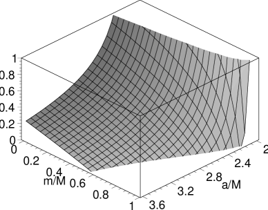
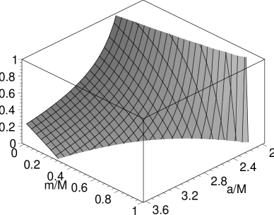
Figure 5: Plots of the stability regions for a dark energy star with constant energy density. We have considered $\omega=-0.5$ and $\omega=-1.25$, in the first and second plots, respectively. The stability regions are given below the surfaces. Qualitatively, one verifies that the stability regions decrease for a decreasing dark energy parameter.

2. Tolman-Matese-Whitman mass function

Consider the Tolman-Matese-Whitman mass function, which represents a monotonic decreasing energy density in the star interior, and the respective “gravity profile”, given by

$$m(r) = \frac{b_{0}r^{3}}{2(1+2b_{0}r^{2})}\,,$$ (49)

$$g(r) = \left(\frac{b_{0}r}{2}\right)\left[\frac{(1+3\omega)+(1+\omega)2b_{0}r^{2}}{(1+b_{0}r^{2})(1+2b_{0}r^{2})}\right]\,.$$ (50)

Note that the constant $b_{0}$ may be expressed in terms of the mass function, as $b_{0}=2m[a^{3}(1-4m/a)]^{-1}$. Now, as $b_{0}$ is considered to be non-negative, by construction, then an additional restriction needs to be imposed, namely, $a>4m(a)$. However, as we are primarily interested in the behavior of the model’s surface layer where the event horizon is expected to form, i.e., $a\gtrsim 2M$, we shall only analyze the domain $0<m/M\leq 1/2$.

For the case of $m(a)<M$, as in the previous example, one may also prove that $d\sigma^{2}/da|_{a_{0}}<0$, so that the stability regions are also dictated by inequality (45). The stability regions are depicted in Fig. 6, for the specific case of $\omega=-0.5$. It is possible to show that the stability regions, for this specific case, are very insensitive to variations in $\omega$. One may prove that the stability configurations slightly increase for high $m/M$, and slightly decrease for relatively low values of $m/M$, for decreasing values of the dark energy parameter $\omega$.

The message that one may extract, as in the previous example, is that stable dark energy stars exist with a transition layer placed sufficiently close to where the event horizon is expected to form, so that the exterior geometry of these stars would be difficult to distinguish from an astrophysical black hole.

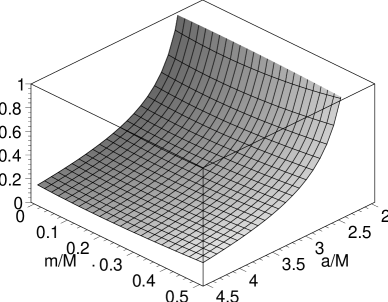
Figure 6: Plot of the stability region for a dark energy star with the Tolman-Matese-Whitman mass function, where we have considered the case of $\omega=-0.5$. The stability region is given below the surface. See the text for details.

V Summary and Conclusion

Although evidence for the existence of black holes is very convincing, a certain amount of scepticism regarding the physical reality of event horizons is still encountered, and it has been argued that despite the fact that observational data do indeed provide strong arguments in favor of event horizons, they cannot fundamentally prove their existence AKL . In part, due to this scepticism, a new picture for an alternative final state of gravitational collapse has emerged, where an interior compact object is matched to an exterior Schwarzschild vacuum spacetime, at or near where the event horizon is expected to form. Therefore, these alternative models do not possess a singularity at the origin and have no event horizon, as its rigid surface is located at a radius slightly greater than the Schwarzschild radius. In particular, the gravastar picture, proposed by Mazur and Mottola Mazur , has an effective phase transition at/near where the event horizon is expected to form, and the interior is replaced by a de Sitter condensate. The latter is then matched to a thick layer, with an equation of state given by $p=\rho$, which is in turn matched to an exterior Schwarzschild solution. A simplified model was then proposed by Visser and Wiltshire VW , where the matching occurred at a thin shell. It has also been argued that there is no way of distinguishing a Schwarzschild black hole from a gravastar from observational data AKL . In this work, a generalization of the gravastar picture was explored, by considering a matching of an interior solution governed by the dark energy equation of state, $\omega\equiv p/\rho<-1/3$, to an exterior Schwarzschild vacuum solution at a junction interface. We emphasize that the motivation for implementing this generalization arises from the fact that recent observations have confirmed an accelerated expansion of the Universe, for which dark energy, a cosmic fluid dictated by an equation of state given by $\omega=p/\rho$ with $\omega<-1/3$, is a possible candidate. We have analyzed several relativistic dark energy stellar configurations by imposing specific choices for the mass function. The first case considered was that of a constant energy density, and the second choice, that of a monotonic decreasing energy density in the star’s interior. We then further explored the dynamical stability of the transition layer of these dark energy stars to linearized spherically symmetric radial perturbations about static equilibrium solutions. It was found that large stability regions do exist, which are located sufficiently close to where the event horizon is expected to form, so that it would be difficult to distinguish the exterior geometry of the dark energy stars, analyzed in this work, from an astrophysical black hole.

The possibility of the existence of dark energy, responsible for the present accelerated expansion of the Universe, has opened up new possibilities in theoretical research. In this context, by extending the notion of a spatially homogeneous dark energy fluid, to inhomogeneous spherically symmetric spacetimes, such as dark energy stars, we point out that the latter have some interesting physical properties. Note that recent fits to supernovae, CMB and weak gravitational lensing data favor an evolving equation of state, with dark energy parameter crossing the phantom divide $\omega=-1$ Vikman ; phantom-divide . Thus, in a rather speculative scenario, one may consider the existence of a dark energy star, with an evolving parameter starting out in the range $-1<\omega<-1/3$, and crossing the phantom divide, $\omega=-1$. A possible approach would be to consider a mixture of interacting non-ideal fluids, as it seems that in a cosmological setting the transition into the phantom regime is physically implausible, for a single scalar field Vikman . One could also apply variations of the approach outlined in Ref. Picon-Lim , where an inhomogeneous spherically symmetric dark energy scalar field was considered, although the latter model does not allow a phantom crossing. Once in the phantom regime, the null energy condition is violated, which physically implies that the negative radial pressure exceeds the energy density. Therefore, an enormous pressure in the center may, in principle, imply a topology change, consequently opening up a tunnel, and converting the dark energy star into a wormhole Morris ; Visser . (However, it is still uncertain whether topology changes will be permitted by an eventual theory of quantum gravity). It has recently been shown that traversable wormholes may, in principle, be supported by phantom energy Sushkov ; Lobo-phantom , which apart from being used as interstellar shortcuts, may induce closed timelike curves with the associated causality violations mty ; Visser . It should be interesting to construct a mathematical model illustrating this conversion, i.e., dark energy star into a wormhole, by considering a time-dependent dark energy parameter, which we leave for a future work. Perhaps not so appealing, one could denote these exotic geometries consisting of dark energy stars (in the phantom regime) and phantom wormholes as phantom stars. As emphasized in the Conclusion of Ref. CFV , we would also like to state our agnostic position relatively to the existence of dark energy stars, however, it is important to understand their general properties to further understand the observational data of astrophysical black holes.

References

- (1) K. Schwarzschild, “Uber das Gravitationsfeld einer Kugel aus inkompressibler Flussigkeit nach der Einsteinschen Theorie,” Sitzber. Deut. Akad. Wiss. Berlin, Kl. Math.-Phys. Tech., 424-434 (1916)
- (2) R. C. Tolman, “Static solutions of Einstein’s field equations for spheres of fluid,” Phys. Rev. 55, 364 (1939).
- (3) J. R. Oppenheimer and G. Volkoff, “On massive neutron cores,” Phys. Rev. 55, 374 (1939).
- (4) C. W. Misner, K. S. Thorne and J. A. Wheeler, 1995, Gravitaiton (W. H. Freeman and company, San Francisco); Ya. B. Zel’dovich and I. D. Novikov, 1974, Relativistic astrophysics, Vol.I: Stars and relativity (University of Chicago Press, Chicago).
- (5) S. Chandrasekhar, “The density of white dwarf stars,” Phil. Mag. 11, 592 (1931); S. Chandrasekhar, “The maximum mass of ideal white dwarfs,” Astrophys. J. 74, 81 (1931).
- (6) W. Baade and F. Zwicky, “Cosmic rays from supernovae,” Proc. Nat. Acad. Sci. U.S. 20, 259 (1934); W. Baade and F. Zwicky, “On supernovae,” Proc. Nat. Acad. Sci. U.S. 20, 254 (1934); W. Baade and F. Zwicky, “Supernovae and cosmic rays,” Phys. Rev. 45, 138 (1934).
- (7) M. Wyman, “Schwarzschild interior solution in an isotropic coordinate system,” Phys. Rev. 70, 74 (1946).
- (8) M. Wyman, “Radially symmetric distributions of matter,” Phys. Rev. 75, 1930 (1949).
- (9) H. A. Buchdahl, “General relativistic fluid spheres,” Phys. Rev. 116, 1027 (1959); H. A. Buchdahl, “General relativistic fluid spheres II: general inequalities for regular spheres,” Astrophys. J. 146, 275 (1966).
- (10) H. Bondi, “Massive spheres in general relativity,” Mon. Not. Roy. Astron. Soc. 282, 303 (1964).
- (11) C. Leibovitz, “Spherically symmetric static solutions of Einstein’s equations,” Phys. Rev. 185, 1664 (1969).
- (12) A. Hewish, S. J. Bell, J. D. H. Pilkington, P. F. Scott and R. A. Collins, “Rotating neutron stars as the origin of the pulsating radio sources,” Nature 218, 731 (1968).
- (13) T. Gold, “Observation of a rapidly pulsating radio source,” Nature 217, 709 (1968).
- (14) R. C. Adams and J. M. Cohen, “Analytic neutron-star models,” Phys. Rev. D 8, 1651 (1973); J. R. Wilson, “Rapidly rotating neutron stars,” Phys. Rev. Lett. 30, 1082 (1973).
- (15) S. S. Bayin, “Solutions of Einstein’s field equations for static fluid spheres,” Phys. Rev. D 18, 2745 (1978).
- (16) S. S. Bayin, “Radiating fluid spheres in general relativity,” Phys. Rev. D 19, 2838 (1979).
- (17) S. S. Bayin, “Anisotropic fluid spheres in general relativity,” Phys. Rev. D 26, 1262 (1982).
- (18) K. S. Thorne, R. H. Price and D. A. Macdonald (editors) Black holes: The membrane paradigm (Yale University Press, New Haven and London).
- (19) J. R. Oppenheimer and H. Snyder, “On Continued Gravitational Contraction,” Phys. Rev. 56, 455 (1939).
- (20) M. A. Abramowicz, W. Kluzniak and J. P. Lasota, “No observational proof of the black-hole event-horizon,” Astron. Astrophys. 396 L31 (2002) [arXiv:astro-ph/0207270].
- (21) P. O. Mazur and E. Mottola, “Gravitational Condensate Stars: An Alternative to Black Holes,” [arXiv:gr-qc/0109035]; P. O. Mazur and E. Mottola, “Dark energy and condensate stars: Casimir energy in the large,” [arXiv:gr-qc/0405111]; P. O. Mazur and E. Mottola, “Gravitational Vacuum Condensate Stars,” Proc. Nat. Acad. Sci. 111, 9545 (2004) [arXiv:gr-qc/0407075].
- (22) G. Chapline, E. Hohlfeld, R. B. Laughlin and D. I. Santiago, “Quantum Phase Transitions and the Breakdown of Classical General Relativity,” Int. J. Mod. Phys. A 18 3587-3590 (2003) [arXiv:gr-qc/0012094].
- (23) I. Dymnikova, “Vacuum nonsingular black hole,” Gen. Rel. Grav. 24, 235 (1992); I. Dymnikova, “The algebraic structure of a cosmological term in spherically symmetric solutions,” Phys. Lett. B472, 33-38 (2000) [arXiv:gr-qc/9912116]; I. Dymnikova, “Cosmological term as a source of mass,” Class. Quant. Grav. 19 725-740 (2002) [arXiv:gr-qc/0112052]; I. Dymnikova, “Spherically symmetric space-time with the regular de Sitter center,” Int. J. Mod. Phys. D 12, 1015-1034 (2003) [arXiv:gr-qc/0304110]; I. Dymnikova and E. Galaktionov, “Stability of a vacuum nonsingular black hole,” Class. Quant. Grav. 22 2331-2358 (2005) [arXiv:gr-qc/0409049].
- (24) M. Visser and D. L. Wiltshire, “Stable gravastars - an alternative to black holes?,” Class. Quant. Grav. 21 1135 (2004) [arXiv:gr-qc/0310107].
- (25) C. Cattoen, T. Faber and M. Visser, “Gravastars must have anisotropic pressures,” (to appear in Class. Quant. Grav.) [arXiv:gr-qc/0505137].
- (26) N. Bilić, G. B. Tupper and R. D. Viollier, “Born-Infeld phantom gravastars,” [arXiv:astro-ph/0503427].
- (27) G. Chapline, “Dark energy stars,” [arXiv:astro-ph/0503200].
- (28) A. Grant et al, “The Farthest known supernova: Support for an accelerating Universe and a glimpse of the epoch of deceleration,” Astrophys. J. 560 49-71 (2001) [arXiv:astro-ph/0104455]; S. Perlmutter, M. S. Turner and M. White, “Constraining dark energy with SNe Ia and large-scale strucutre,” Phys. Rev. Lett. 83 670-673 (1999) [arXiv:astro-ph/9901052].
- (29) C. L. Bennett et al, “First year Wilkinson Microwave Anisotropy Probe (WMAP) observations: Preliminary maps and basic results,” Astrophys. J. Suppl. 148 1 (2003) [arXiv:astro-ph/0302207]; G. Hinshaw et al, “First year Wilkinson Microwave Anisotropy Probe (WMAP) observations: The angular power spectrum,” Astrophys. J. Suppl. 148 135 (2003) [arXiv:astro-ph/0302217].
- (30) I. Brevik, S. Nojiri, S. D. Odintsov and L. Vanzo, “Entropy and universality of Cardy-Verlinde formula in dark energy universe,” Phys. Rev. D 70 043520 (2004) [arXiv:hep-th/0401073]; S. Nojiri and S. D.Odintsov, “The final state and thermodynamics of dark energy universe,” Phys. Rev. D 70 103522 (2004) [arXiv:hep-th/0408170].
- (31) R. R. Caldwell, M. Kamionkowski and N. N. Weinberg, “Phantom Energy and Cosmic Doomsday,” Phys. Rev. Lett. 91 071301 (2003) [arXiv:astro-ph/0302506].
- (32) S. Sushkov, “Wormholes supported by a phantom energy,” Phys. Rev. D 71, 043520 (2005) [arXiv:gr-qc/0502084].
- (33) F. S. N. Lobo, “Phantom energy traversable wormholes,” Phys. Rev. D 71, 084011 (2005) [arXiv:gr-qc/0502099].
- (34) E. Babichev, V. Dokuchaev and Yu. Eroshenko , “Black hole mass decreasing due to phantom energy accretion,” Phys. Rev. Lett. 93 021102 (2004) [arXiv:gr-qc/0402089].
- (35) A. Vikman, “Can dark energy evolve to the Phantom?,” Phys. Rev. D 71 023515 (2005) [arXiv:astro-ph/0407107].
- (36) B. Feng, X. Wang and X. Zhang, “Dark Energy Constraints from the Cosmic Age and Supernova,” Phys. Lett. B607 35-41 (2005) [arXiv:astro-ph/0404224]; Z. Guo, Y. Piao, X. Zhang and Y. Zhang, “Cosmological evolution of a quintom model of dark energy,” Phys. Lett. B608 177-182 (2005) [arXiv:astro-ph/0410654]; X.F. Zhang, H. Li, Y. Piao Z. and X. Zhang, “Two-field models of dark energy with equation of state across ,” [arXiv:astro-ph/0501652]; L. Perivolaropoulos, “Constraints on linear-negative potentials in quintessence and phantom models from recent supernova data,” Phys.Rev. D 71 063503 (2005), [arXiv:astro-ph/0412308]; H. Wei and R. G. Cai, “Hessence: A New View of Quintom Dark Energy,” Class. Quant. Grav. 22 3189-3202 (2005) [arXiv:hep-th/0501160]; M. Li, B. Feng and X. Zhang, “A Single Scalar Field Model of Dark Energy with Equation of State Crossing ,” [arXiv:hep-ph/0503268]; H. Stefancic, “Dark energy transition between quintessence and phantom regimes - an equation of state analysis,” Phys. Rev. D 71 124036 (2005) [arXiv:astro-ph/0504518]; A. Anisimov, E. Babichev and A. Vikman, “B-Inflation,” JCAP 0506 006 (2005) [arXiv:astro-ph/0504560]; B. Wang, Y. Gong and E. Abdalla, “Transition of the dark energy equation of state in an interacting holographic dark energy model,” [arXiv:hep-th/0506069]; S. Nojiri and S. D. Odintsov, “Unifying phantom inflation with late-time acceleration: scalar phantom-non-phantom transition model and generalized holographic dark energy,” [arXiv:hep-th/0506212]; I.Ya. Aref’eva, A.S. Koshelev, S.Yu. Vernov, “Crossing of the Barrier by D3-brane Dark Energy Model,” [arXiv:astro-ph/0507067]; Gong-Bo Zhao, Jun-Qing Xia, Mingzhe Li, Bo Feng and Xinmin Zhang, “Perturbations of the Quintom Models of Dark Energy and the Effects on Observations,” [arXiv:astro-ph/0507482]. S. Tsujikawa, “Reconstruction of general scalar-field dark energy models,” [arXiv:astro-ph/0508542].
- (37) C. Armendariz-Picon and E. A. Lim, “Haloes of k-Essence,” [arXiv:astro-ph/0505207].
- (38) F. S. N. Lobo and P. Crawford, “Stability analysis of dynamic thin shells,” Class. Quant. Grav. 22, 4869 (2005), [arXiv:gr-qc/0507063].
- (39) F. S. N. Lobo, “Stability of phantom wormholes,” Phys. Rev. D 71, 124022 (2005) [arXiv:gr-qc/0506001].
- (40) S. Nojiri and S. D. Odintsov, “Inhomogeneous Equation of State of the Universe: Phantom Era, Future Singularity and Crossing the Phantom Barrier,” Phys. Rev. D 72, 023003 (2005) [arXiv:gr-qc/0306109].
- (41) D. Martin and M. Visser, “Bounds on the interior geometry and pressure profile of static fluid spheres,” Class. Quant. Grav. 20 3699 (2003) [arXiv:gr-qc/0306038].
- (42) D. Martin and M. Visser, “Algorithmic construction of static perfect fluid spheres,” Phys. Rev. D 69, 104028 (2004) [arXiv:gr-qc/0306109].
- (43) M. Morris and K.S. Thorne, “Wormholes in spacetime and their use for interstellar travel: A tool for teaching General Relativity,” Am. J. Phys. 56, 395 (1988).
- (44) J. J. Matese and P. G. Whitman, “New methods for extracting equilibrium configurations in general relativity,” Phys. Rev. D 22 1270-1275 (1980).
- (45) M. R. Finch and J. E. F. Skea, “A realistic stellar model based on the ansatz of Duorah and Ray,” Class. Quant. Grav. 6 467-476 (1989).
- (46) M. K. Mak and T. Harko, “Anisotropic Stars in General Relativity,” Proc. Roy. Soc. Lond. A459, 393-408 (2003) [arXiv:gr-qc/0110103]; M. K. Mak and T. Harko, “Anisotropic relativistic stellar models,” Annalen Phys. 11, 3-13 (2003) [arXiv:gr-qc/0302104].
- (47) J. P. S. Lemos, F. S. N. Lobo and S. Q. de Oliveira, “Morris-Thorne wormholes with a cosmological constant,” Phys. Rev. D 68, 064004 (2003) [arXiv:gr-qc/0302049]. J. P. S. Lemos and F. S. N. Lobo, “Plane symmetric traversable wormholes in an anti-de Sitter background,” Phys. Rev. D 69 (2004) 104007 [arXiv:gr-qc/0402099]; F. S. N. Lobo, “Surface stresses on a thin shell surrounding a traversable wormhole,” Class. Quant. Grav. 21 4811 (2004) [arXiv:gr-qc/0409018]; F. S. N. Lobo, “Energy conditions, traversable wormholes and dust shells,” Gen. Rel. Grav. 37, 2023-2038 (2005) [arXiv:gr-qc/0410087].
- (48) J. Guven and N. O’ Murchadha, “Bounds on for static spherical objects,” Phys. Rev. D 60 084020 (1999) [arXiv:gr-qc/9903067]; S. Rahman and M. Visser, “Spacetime geometry of static fluid spheres,” Class. Quant. Grav. 19 935 (2002) [arXiv:gr-qc/0103065]; B. V. Ivanov, “Maximum bounds on the surface redshift of anisotropic stars,” Phys. Rev. D 65 104011 (2002) [arXiv:gr-qc/0201090].
- (49) W. Israel, “Singular hypersurfaces and thin shells in general relativity,” Nuovo Cimento 44B, 1 (1966); and corrections in ibid. 48B, 463 (1966).
- (50) E. Poisson and M. Visser, “Thin-shell wormholes: Linearization stability,” Phys. Rev. D 52 7318 (1995) [arXiv:gr-qc/9506083]; M. Ishak and K. Lake, “Stability of transparent spherically symmetric thin shells and wormholes,” Phys. Rev. D 65 044011 (2002); E. F. Eiroa and G. E. Romero, “Linearized stability of charged thin-shell wormoles,” Gen. Rel. Grav. 36, 651 (2004), [arXiv:gr-qc/0303093]; F. S. N. Lobo and P. Crawford, “Linearized stability analysis of thin-shell wormholes with a cosmological constant,” Class. Quant. Grav. 21, 391 (2004) [arXiv:gr-qc/0311002].
- (51) Visser M 1995 Lorentzian Wormholes: From Einstein to Hawking (American Institute of Physics, New York)
- (52) M. S. Morris, K. S. Thorne and U. Yurtsever, “Wormholes, Time Machines and the Weak Energy Condition,” Phy. Rev. Lett. 61, 1446 (1988).