Spacetime metric from local and linear electrodynamics: a new axiomatic scheme

Abstract

We consider spacetime to be a 4-dimensional differentiable manifold that can be split locally into time and space. No metric, no linear connection are assumed. Matter is described by classical fields/fluids. We distinguish electrically charged from neutral matter. Electric charge and magnetic flux are postulated to be conserved. As a consequence, the inhomogeneous and the homogeneous Maxwell equations emerge expressed in terms of the excitation $H=({\cal H},{\cal D})$ and the field strength ${F}=(E,B)$, respectively. $H$ and $F$ are assumed to fulfill a local and linear “spacetime relation” with 36 constitutive functions. The propagation of electromagnetic waves is considered under such circumstances in the geometric optics limit. We forbid birefringence in vacuum and find the light cone including its Lorentzian signature. Thus the conformally invariant part of the metric is recovered. If one sets a scale, one finds the pseudo-Riemannian metric of spacetime.

Invited lecture, 339th WE Heraeus Seminar on Special Relativity
Potsdam, Germany, 13-18 February 2005

1 Introduction

The neutrinos, in the standard model of elementary particle physics, are assumed to be massless. By the discovery of the neutrino oscillations, this assumption became invalidated. The neutrinos are massive, even though they carry, as compared to the electron, only very small masses. Then the photon is left as the only known massless and free elementary particle. The gluons do not qualify in this context since they are confined and cannot exist as free particles under normal circumstances.

Consequently, the photon is the only particle that is directly related to the light cone $g_{ij}dx^{i}\otimes dx^{j}=0$ and that can be used for an operational definition of the light cone; here $g_{ij}$ is the metric of spacetime, $dx^{i}$ a coordinate differential, and $i,j=0,1,2,3$. We are back — as the name light cone suggests anyway — to an electromagnetic view of the light cone. Speaking in the framework of classical optics, the light ray would then be the elementary object with the help of which one can span the light cone. We take “light ray” as synonymous for radar signals, laser beams, or electromagnetic rays of other wavelengths. It is understood that classical optics is a limiting case, for short wavelengths, of classical Maxwell-Lorentz electrodynamics.

In other words, if we assume the framework of Maxwell-Lorentz electrodynamics, we can derive, in the geometric optics limit, light rays and thus the light cone, see Perlick Perlick00 and the literature given there. However, the formalism of Maxwell-Lorentz electrodynamics is interwoven with the Riemannian metric $g_{ij}$ in a nontrivial way. Accordingly, in the way sketched, one can never hope to find a real derivation of the light cone.

Therefore, we start from the premetric form of electrodynamics, that is, a metric of spacetime is not assumed. Nevertheless, we can derive the generally covariant Maxwell equations, expressed in terms of the excitation $H=({\cal H},{\cal D})$ and the field strength ${F}=(E,B)$, from the conservation laws of electric charge and magnetic flux. We assume a local and linear spacetime relation between $H$ and $F$. Then we can solve the Maxwell equations. In particular, we can study the propagation of electromagnetic waves, and we can consider the geometrical optics limit. In this way, we derive the light rays that are spanning the light cone. In general, we find a quartic wave covector surface (similar as in a crystal) that only reduces to the pseudo-Riemannian light cone of general relativity if we forbid birefringence (double refraction) in vacuum. Hence, in the framework of premetric electrodynamics, the local and linear spacetime relation, together with a ban on birefringence in vacuum, yields the pseudo-Riemannian light cone of general relativity. Accordingly, the geometrical structure of a Riemannian spacetime is derived from purely electromagnetic data. We consider that as our contribution to the Einstein year 2005, and we hope that going beyond the geometrical optics limit will yield better insight into the geometry of spacetime.

The axiomatic scheme that we are going to present here is already contained in our book Birkbook where also references to earlier work and more details can be found. In the meantime we learnt from the literature that appeared since 2003 (see, e.g., Delphenich Delphenich1 ; Delphenich2 , Itin Itin , Kaiser Kaiser , Kiehn Kiehn04 , and Lindell & Sihvola Lindell ; LindSihv2004a ) and improved our derivation of the light cone, simplified it, made it more transparent (see, e.g., ourmonopole ; PostCon ; Laemmerzahl04 ; skewon ; measure ). The formalism and the conventions we take from Birkbook .

2 Spacetime

In our approach, we start from a 4-dimensional spacetime manifold that is just a continuum which can be decomposed locally in (1-dimensional) time and (3-dimensional) space. It carries no metric and it carries no (linear or affine) connection. As such it is inhomogeneous. It doesn’t make sense to assume that a vector field is constant in this continuum. Only the constancy of a scalar field is uniquely defined. Also a measurement of temporal or spatial intervals is still not defined since a metric is not yet available.

In technical terms, the spacetime is a 4-dimensional connected, Hausdorff, paracompact, and oriented differential manifold. On such a manifold, we assume the existence of a foliation: The spacetime can be decomposed locally into three-dimensional folios labeled consecutively by a monotonically increasing “prototime” parameter $\sigma$, see Fig. 1.

Figure 1: Local spacetime foliation, see Birkbook .

A vector field $n$, transverse to the foliation, is normalized by $n\rfloor d\sigma={\cal L}_{n}\sigma=1$. Accordingly, we find for the dimensions $[n]=[\sigma]^{-1}=t^{-1}$, where $t$ denotes the dimension of time.

We can decompose any exterior form $\Psi$ in “time” and “space” pieces. The part longitudinal to the vector $n$ reads

$$^{\bot}\Psi:=d\sigma\wedge\Psi_{\bot}\,,\qquad\Psi_{\bot}:={n}\rfloor\Psi\,,$$ (1)

the part transversal to the vector $n$

$$\underline{\Psi}:=(1\;-\;^{\bot})\Psi={n}\rfloor(d\sigma\wedge\Psi)\,,\quad{n}\rfloor\,\underline{\Psi}\equiv 0\,.$$ (2)

Putting these two parts together, we have the space-time decomposition

$$\Psi=\,^{\bot}\Psi+\underline{\Psi}=d\sigma\wedge\Psi_{\bot}+\underline{\Psi}\,,$$ (3)

with the absolute dimensions $[\Psi_{\bot}]=[\Psi]\,t^{-1}$ and $[\underline{\Psi}]=[\Psi]$.

The 3-dimensional exterior derivative is defined by $\underline{d}:=n\rfloor(d\sigma\wedge d)$. We can use the notion of the Lie derivative of a $p$-form $\Psi$ along a vector field $\xi$, i.e., ${\cal L}_{\xi}\Psi:=\xi\rfloor d\Psi+d(\xi\rfloor\Psi)$, and can introduce the derivative of a transversal field $\underline{\Psi}$ with respect to prototime as

$$\dot{\underline{\Psi}}:={\cal L}_{n}\underline{\Psi}\,.$$ (4)

3 Matter — electrically charged and neutral

We assume that spacetime is “populated” with classical matter, either described by fields and/or by fluids. In between the agglomerations of matter, there may also exist vacuum.

Matter is divided into electrically charged and neutral matter. Turning to the physics of the former, we assume that on the spatial folios of the manifold we can determine an electric charge $Q$ as a 3-dimensional integral over a charge density and a magnetic flux $\Phi$ as a 2-dimensional integral over a flux density.

This is at the bottom of classical electrodynamics: Spacetime is filled with matter that is characterized by charge $Q$ and by magnetic flux $\Phi$. For neutral matter both vanish. The absolute dimension of charge will be denoted by $q$, that of magnetic flux by $\phi$ = [action/charge] = $h/q$, with $h$ as the dimension of action.

4 Electric charge conservation

One can catch single electrons and single protons in traps and can count them individually. Thus, the electric charge conservation is a fundamental law of nature, valid in macro- as well as in micro-physics. Accordingly, it is justified to introduce the absolute dimension of charge $q$ as a new and independent concept.

Let us define, in 4-dimensional spacetime, the electrical current 3-form $J$, with dimension $[J]=q$. Its integral over an arbitrary 3-dimensional spacetime domain yields the total charge contained therein: $Q=\int_{\Omega_{3}}J$. Accordingly, the local form of charge conservation (Axiom 1) reads:

$$d\,J=0\,.$$ (5)

This law is metric-independent since it is based on a counting procedure for the elementary charges. Using a foliation of spacetime, we can decompose the current $J$ into the 2-form of the electric current density $j$ and the 3-form $\rho$ of the electric charge density:

$$J=-j\wedge d\sigma+\rho\,.$$ (6)

Then (5) can be rewritten as the continuity equation:

$$\dot{\rho}+\underline{d}\,j=0.$$ (7)

Both versions of charge conservation, eqs.(5) and (7), can also be formulated in an integral form.

5 Charge active: excitation

Electric charge was postulated to be conserved in all regions of spacetime. If spacetime is topologically sufficiently trivial, we find, as consequence of (5), that $J$ has to be exact:

$$J=d\,H\,.$$ (8)

This is the inhomogeneous Maxwell equation in its premetric form. The electromagnetic excitation 2-form $H$, with $[H]=[J]=q$, is measurable with the help of ideal conductors and superconductors and thus has a direct operational significance.

By decomposing $H$ into time and space, we obtain the electric excitation 2-form ${{\cal D}}$ (historical name: “dielectric displacement”) and the magnetic excitation 1-form ${{\cal H}}$ (“magnetic field”):

$$H=-{\cal H}\wedge d\sigma+{\cal D}\,.$$ (9)

Substituting (9) into (8), we recover the pair of the 3-dimensional inhomogeneous Maxwell equations

$$d\,H=J\>\,\,\begin{cases}\hskip 30.0pt\underline{d}\,{\cal D}\>=\rho\,,\\ -\,\dot{\cal D}+\underline{d}\,{\cal H}\>=j\,.\end{cases}$$ (10)

6 Charge passive: field strength

With the derivation of the inhomogeneous Maxwell equations the information contained in Axiom 1 is exhausted. As is evident from the Coulomb-Gauss law $\underline{d}\,{\cal D}=\rho$, it is the active character of $\rho$ that plays a role in this inhomogeneous Maxwell equation: The charge density $\rho$ is the source of ${\cal D}$ (and, analogously, the current density $j$ that of ${\cal H}$).

Since we search for new input, it is near at hand to turn to the passive character of charge, that is, to wonder what happens when a test charge is put in an electromagnetic field. In the purely electric case with a test charge $e$, we have

$${F}_{a}\sim e\,{E_{a}}\,,\$$ (11)

with ${F}_{a}$ and $E_{a}$ as components of the covectors of force and electric field strength, respectively. The simplest relativistic generalization for defining the electromagnetic field is then of the type

$${\rm force\>\>density}\sim{\rm field\>\>strength}\times{\rm charge\>\>current\>\>density}\,.$$ (12)

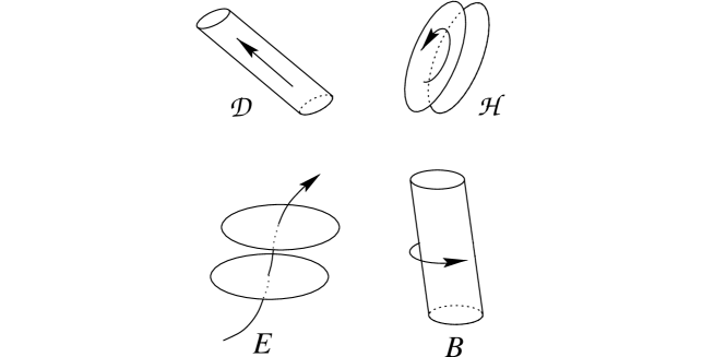
Figure 2: Faraday-Schouten pictograms of the electromagnetic field, see Birkbook . The electric excitation $\cal D$ is a twisted 2-form, the magnetic excitation $\cal H$ a twisted 1-form. The electric field strength $E$ is a 1-form and the magnetic field strength $B$ a 2-form, both without twist.

Accordingly, with the force density covector (or 1-form) $f_{\alpha}$, we can formulate Axiom 2 as

$$f_{\alpha}=(e_{\alpha}\rfloor F)\wedge J\,.$$ (13)

Here $e_{\alpha}$ is a local frame, with $\alpha=0,1,2,3$. Axiom 2 provides an operational definition of the electromagnetic field strength 2-form $F$, the absolute dimension of which turns out to be $[F]=h/q$. Its $1+3$ decomposition

$$F=E\wedge d\sigma+B\,,$$ (14)

introduces the electric field strength 1-form $E$ and the magnetic field strength 2-form $B$, see Fig.2. If we substitute (14) and (6) into (13), we recover, for $\alpha=1,2,3$, the Lorentz force density.

7 Magnetic flux conservation

The field strength $F$, as a 2-form, can be integrated over a 2-dimensional area $\Omega_{2}$ in 4-dimensional spacetime. This yields the total magnetic flux $\Phi$ piercing through this area: $\Phi=\int_{\Omega_{2}}F$. In close analogy to electric charge conservation, we assume that also the flux is conserved. Then, in local form, magnetic flux conservation (Axiom 3) reads

$$d\,F=0\>\,\,\begin{cases}\qquad\underline{d}\,B\>=0\,,\\ \dot{B}+\underline{d}\,E\>=0\,.\end{cases}$$ (15)

The Faraday induction law and the sourcelessness of $B$ are the two consequences of $dF=0$. In this sense, Axiom 3 has a firm experimental underpinning.

8 Premetric electrodynamics

…is meant to be the “naked” or “featureless” spacetime manifold, without metric and without connection, together with the Maxwell equations $dH=J,\,dF=0$, the Lorentz force formula, and the electromagnetic energy-momentum current to be discussed below, see (20). We stress that the Poincaré group and special relativity have nothing to do with the foundations of electrodynamics as understood here in the sense of the decisive importance of the underlying generally covariant conservation laws of charge (Axiom 1) and flux (Axiom 3). Historically, special relativity emerged in the context of an analysis of the electrodynamics of moving bodies Einstein05 ; Dover1952 , but within the last 100 years classical electrodynamics had a development of its own and its structure is now much better understood than it was 100 years ago. Diffeomorphism invariance was recognized to be of overwhelming importance. Poincaré invariance turned out to play a secondary role only.

Of course, premetric electrodynamics so far does not represent a complete physical theory. The excitation $H$ does not yet communicate with the field strength $F$. Only by specifying a “spacetime” relation between $H$ and $F$ (the constitutive law of the spacetime manifold), only thereby we recover — under suitable conditions — our normal Riemannian or Minkowskian spacetime which we seem to live in. In this sense, a realistic spacetime — and thus an appropriate geometry thereof — emerges only by specifying additionally a suitable spacetime relation on the featureless spacetime.

As explained, Axiom 1, Axiom 2, Axiom 3, together with Axiom 4 on energy-momentum, constitute premetric electrodynamics. Let us display the first three axions here again, but now Axiom 1 and Axiom 3 in in the more general integral version. For any submanifolds $C_{3}$ and $C_{2}$ that are closed, i.e., $\partial C_{3}=0$ and $\partial C_{2}=0$, the axioms read

$$\oint\limits_{C_{3}}J=0\,,\qquad f_{\alpha}=(e_{\alpha}\rfloor F)\wedge J\,,\qquad\oint\limits_{C_{2}}F=0\,.$$ (16)

By de Rham’s theorem we find the corresponding differential versions

$$d\,J = 0\,,\qquad f_{\alpha}=(e_{\alpha}\rfloor F)\wedge J\,,\qquad dF=0\,,$$ (17)

$$J = d\,H\,,\qquad\qquad\qquad\quad\qquad\qquad\hskip 3.0ptF=dA\,.$$ (18)

The physical interpretation of the quantities involved is revealed via their $(1+3)$-decompositions (6), (9), (14), and $A=-\varphi d\sigma+{\cal A}$, see Fig.3.

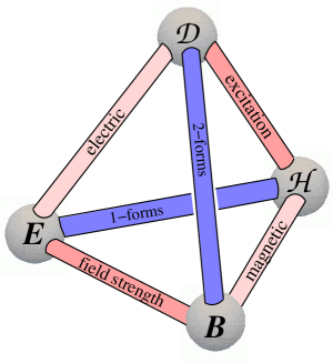
Figure 3: Different aspects of the electromagnetic field. The four quantities ${\cal H},{\cal D},E,B$ constitute the electromagnetic field. The excitations ${\cal H},{\cal D}$ are extensive quantities (how much?), the field strengths $E,B$ intensive quantities (how strong?).

Let us now turn to the energy-momentum question. Using the properties of the exterior differential, we can rewrite the Lorentz force density (13) as

$$f_{\alpha}=(e_{\alpha}\rfloor F)\wedge J=d\,^{\rm k}\!\Sigma_{\alpha}+X_{\alpha}\,.$$ (19)

Here the kinematic energy-momentum 3-form of the electromagnetic field, a central result in the premetric electrodynamics, reads (Axiom 4)

$${}^{\rm k}\!\Sigma_{\alpha}:={\frac{1}{2}}\left[F\wedge(e_{\alpha}\rfloor H)-H\wedge(e_{\alpha}\rfloor F)\right]\,.$$ (20)

The remaining force density 4-form turns out to be

$$X_{\alpha}:=-{\frac{1}{2}}\left(F\wedge{\cal L}_{e_{\alpha}}H-H\wedge{\cal L}_{e_{\alpha}}F\right)\,.$$ (21)

The absolute dimension of ${}^{\rm k}\!\Sigma_{\alpha}$ and of ${X}_{\alpha}$ is $h/\ell$, where $\ell$ denotes the dimension of length. [Provided, additionally, a linear connection is given with the covariant differential $D$, then

$$f_{\alpha}=D^{\rm k}\!\Sigma_{\alpha}+\widehat{X}_{\alpha}\,,$$ (22)

with the new supplementary force density

$$\widehat{X}_{\alpha}={\frac{1}{2}}\left(H\wedge{\hbox{\L}}_{e_{\alpha}}F-F\wedge{\hbox{\L}}_{e_{\alpha}}H\right)\,,$$ (23)

which contains the covariant Lie derivative. In general relativity theory, $\widehat{X}_{\alpha}$ eventually vanishes for the standard Maxwell-Lorentz electrodynamics.]

9 The excitation is local and linear in the field strength

The system of the Maxwell equations $dH=J\,,\,dF=0$ is apparently underdetermined. It gets predictive power only when we supplement it with a spacetime (or constitutive) relation between the excitation and the field strength. As Axiom 5, we postulate a general local and linear spacetime relation

$$H=\kappa(F)\,,\qquad H_{ij}={\frac{1}{2}}\,\kappa_{ij}{}^{kl}\,F_{kl}\,.$$ (24)

Here excitation and field strength decompose according to $H=H_{ij}\,dx^{i}\wedge dx^{j}/2$ and $F=F_{ij}\,dx^{i}\wedge dx^{j}/2$, respectively. The constitutive tensor $\kappa$, as 4th rank tensor with 36 independent components, has to be space and time dependent since constant components would not have a generally covariant meaning on the naked spacetime manifold we consider.

Let us decompose $\kappa_{ij}{}^{kl}$ into irreducible pieces. In the premetric framework we can only perform a contraction. A first contraction yields

$$\kappa_{i}{}^{k}:=\kappa_{il}{}^{kl}\,\quad{\rm(16\;independent\;functions)}\,,$$ (25)

a second one

$$\kappa:=\kappa_{k}{}^{k}=\kappa_{kl}{}^{kl}\,\quad\hbox{(1 pseudo-scalar function)}\,.$$ (26)

Then, introducing the traceless piece

$$\not\!\kappa_{i}{}^{k}:=\kappa_{i}{}^{k}-{\frac{1}{4}}\,\kappa\,\delta_{i}^{k}\,\quad\hbox{(15 functions)}\,,$$ (27)

we can rewrite the original constitutive tensor as

$$\kappa_{ij}{}^{kl} = {}^{(1)}\kappa_{ij}{}^{kl}+{}^{(2)}\kappa_{ij}{}^{kl}+{}^{(3)}\kappa_{ij}{}^{kl}$$ (28)

$$= {}^{(1)}\kappa_{ij}{}^{kl}+2\!\not\!\kappa_{[i}{}^{[k}\,\delta_{j]}^{l]}+{\frac{1}{6}}\,\kappa\,\delta_{[i}^{k}\delta_{j]}^{l}.$$

The skewon and the axion fields are conventionally defined by

$$\!\not\!S_{i}{}^{j}=-\,{\frac{1}{2}}\!\not\!\kappa_{i}{}^{j},\qquad\alpha={\frac{1}{12}}\,\kappa.$$ (29)

Substituting (28) into (24) and using (29), we obtain the spacetime relation explicitly:

$$H_{ij}={\frac{1}{2}}\,^{(1)}\kappa_{ij}{}^{kl}\,F_{kl}+2\,\!\not\!S_{[i}{}^{k}F_{j]k}+\alpha\,F_{ij}\,.$$ (30)

The principal (or the metric-dilaton) part ${}^{(1)}\kappa_{ij}{}^{kl}$ of the constitutive tensor with 20 independent components will eventually be expressed in terms of the metric (thereby cutting the 20 components in half). [In standard Maxwell-Lorentz electrodynamics

$${}^{(1)}\kappa_{ij}{}^{kl}=\lambda_{0}\,\sqrt{-g}\,\hat{\epsilon}_{ijmn}\,g^{mk}g^{nl}\,,\quad{\!\not\!S}_{i}{}^{k}=0\,,\quad\alpha=0.]$$ (31)

The principal part ${}^{(1)}\kappa_{ij}{}^{kl}$ must be non-vanishing in order to allow for electromagnetic wave propagation in the geometrical optics limit, see the next section. The skewon part ${\not\!S}_{i}{}^{k}$ with its 15 components was proposed by us. We put forward the hypothesis that such a field exists in nature. Finally, the axion part $\alpha$ had already been introduced in elementary particle physics in a different connection but with the same result for electrodynamics, see, e.g., Wilczek’s axion electrodynamics Wilczek87 and the references given there.

The spacetime relation we are discussing here is the constitutive relation for spacetime, i.e., for the vacuum. However, one has analogous structures for a medium described by a local and linear constitutive law. The skewon piece in this framework corresponds to chiral properties of the medium inducing optical activity, see Lindell et al. Lindell94 , whereas the concept of an axion piece has been introduced by Tellegen Tellegen1948 ; Tellegen1956/7 for a general medium, by Dzyaloshinskii Dzyaloshinskii specifically for Cr₂O₃, and by Lindell & Sihvola LindSihv2004a in the form of the so-called perfect electromagnetic conductor (PEMC). Recently, Lindell Lindell2005 discussed the properties of a skewon-axion medium.

The following alternative representation of the constitutive tensor is useful in many derivations and for a comparison with literature, see Post Post ,

$$\chi^{ijkl}:={\frac{1}{2}}\,\epsilon^{ijmn}\,\kappa_{mn}{}^{kl}\,,$$ (32)

with

$$\chi^{ijkl}={}\underbrace{{}^{(1)}\chi^{ijkl}}_{20,\,\text{principal}}+\underbrace{\epsilon^{ijm[k}\!\not\!S_{m}{}^{l]}-\epsilon^{klm[i}\!\not\!S_{m}{}^{j]}}_{15,\,\text{skewon}}+\underbrace{\epsilon^{ijkl}\,\alpha\;}_{1,\,\text{axion}}\,.$$ (33)

It is convenient to consider the excitation $H$ and the field strength $F$ as 6-vectors, each comprising a pair of two 3-vectors. The spacetime relation then reads

$$\left(\begin{array}[]{c}{\cal H}_{a}\\ {\cal D}^{a}\end{array}\right)=\left(\begin{array}[]{cc}{{\mathfrak{C}}}^{b}{}_{a}&{{\mathfrak{B}}}_{ba}\\ {{\mathfrak{A}}}^{ba}&{{\mathfrak{D}}}_{b}{}^{a}\end{array}\right)\left(\begin{array}[]{c}-E_{b}\\ {B}^{b}\end{array}\right)\,.$$ (34)

Accordingly, the constitutive tensors are represented by the $6\times 6$ matrices

$$\kappa_{I}{}^{K}=\left(\begin{array}[]{cc}{{\mathfrak{C}}}^{b}{}_{a}&{{\mathfrak{B}}}_{ba}\\ {{\mathfrak{A}}}^{ba}&{{\mathfrak{D}}}_{b}{}^{a}\end{array}\right)\,,\qquad\chi^{IK}=\left(\begin{array}[]{cc}{\mathfrak{B}}_{ab}&{\mathfrak{D}}_{a}{}^{b}\\ {\mathfrak{C}}^{a}{}_{b}&{\mathfrak{A}}^{ab}\end{array}\right)\,.$$ (35)

The $3\times 3$ matrices $\mathfrak{A,B,C,D}$ are defined by

$${\mathfrak{A}}^{ba} := \chi^{0a0b}\,,\qquad{\mathfrak{B}}_{ba}:=\frac{1}{4}\,\hat{\epsilon}_{acd}\,\hat{\epsilon}_{bef}\,\chi^{cdef}\,,$$ (36)

$${\mathfrak{C}}^{a}{}_{b} := \frac{1}{2}\,\hat{\epsilon}_{bcd}\,\chi^{cd0a}\,,\qquad{\mathfrak{D}}_{a}{}^{b}:=\frac{1}{2}\,\hat{\epsilon}_{acd}\,\chi^{0bcd}\,,$$ (37)

or explicitly, recalling the irreducible decomposition (33),

$${\mathfrak{A}}^{ab} = -\varepsilon^{ab}-\epsilon^{abc}\,\!\not\!S_{c}{}^{0},\qquad{\mathfrak{B}}_{ab}=\mu_{ab}^{-1}+\hat{\epsilon}_{abc}\,\!\not\!S_{0}{}^{c},$$ (38)

$${\mathfrak{C}}^{a}{}_{b} = \>\;\gamma^{a}{}_{b}\,-(\!\not\!S_{b}{}^{a}-\delta_{b}^{a}\,\!\not\!S_{c}{}^{c})+\alpha\,\delta_{b}^{a},$$ (39)

$${\mathfrak{D}}_{a}{}^{b} = \>\;\gamma^{b}{}_{a}\,+(\!\not\!S_{a}{}^{b}-\delta_{a}^{b}\,\!\not\!S_{c}{}^{c})+\alpha\,\delta_{a}^{b}.$$ (40)

The constituents of the principal part are the permittivity tensor $\varepsilon^{ab}=\varepsilon^{ba}$, the impermeability tensor $\mu^{-1}_{ab}=\mu_{ba}^{-1}$, and the magnetoelectric cross-term $\gamma^{a}{}_{b}$, with $\gamma^{c}{}_{c}=0$ (Fresnel-Fizeau effect). The skewon ${\not\!S}_{b}{}^{a}$ and the axion $\alpha$ describe electric and magnetic Faraday effects and (in the last two relations) optical activity. If we substitute (38),(39),(40) into (34), we find a 3-dimensional explicit form of our Axiom 5 formulated in (24):

$${\cal D}^{a}\! =\! \left(\varepsilon^{ab}\,-\epsilon^{abc}\not\!S_{c}{}^{0}\right)E_{b}\,+\left(\hskip 9.0pt\gamma^{a}{}_{b}+\not\!S_{b}{}^{a}-\delta_{b}^{a}\not\!S_{c}{}^{c}\right){B}^{b}+\alpha B^{a}\,,$$ (41)

$${\cal H}_{a}\! =\! \left(\mu_{ab}^{-1}-\hat{\epsilon}_{abc}\not\!S_{0}{}^{c}\right){B}^{b}+\left(-\gamma^{b}{}_{a}+\not\!S_{a}{}^{b}-\delta_{a}^{b}\not\!S_{c}{}^{c}\right)E_{b}-\alpha\,E_{a}\,.$$ (42)

10 Propagation of electromagnetic rays (“light”)

After the spacetime relation (Axiom 5) has been formulated, we have a complete set of equations describing the electromagnetic field. We can now study the propagation of electromagnetic waves à la Hadamard. The sourceless Maxwell equations read

$$dH=0\,,\quad dF=0\,.$$ (43)

In the geometric optics approximation (equivalently, in the Hadamard approach) an electromagnetic wave is described by the propagation of a discontinuity of the electromagnetic field. The surface of discontinuity $S$ is defined locally by a function $\Phi$ such that $\Phi=const$ on $S$. The jumps $[\;]$ of the electromagnetic quantities across $S$ and the wave covector $q:=d\Phi$ then satisfy the geometric Hadamard conditions:

$$[H]=0\,,\;[dH]=q\wedge h=0\;\qquad\Rightarrow\qquad h=q\wedge c\,,$$ (44)

$$\,[F]=0\,,\;[dF]=q\wedge f=0\;\qquad\Rightarrow\qquad f=q\wedge a\,.$$ (45)

Here $c$ and $a$ are arbitrary 1-forms.

We use the spacetime relation and find for the jumps of the field derivatives

$$h=\kappa(f)=\widetilde{\kappa}(f)+\alpha f\,,$$ (46)

with $\widetilde{\kappa}:=\,^{(1)}\kappa+{}^{(2)}\kappa$. Accordingly,

$$q\wedge h={q\wedge\widetilde{\kappa}(q\wedge a)=0\,}.$$ (47)

This equation is a 3-form with 4 components. We have to solve it with respect to $a$. As a first step, we have to remove the gauge freedom $a\rightarrow a+q\,\varphi$ present in (47). We choose the gauge $\vartheta^{\hat{0}}\stackrel{{\scriptstyle*}}{{=}}q$. After some heavy algebra, we find (see Birkbook for details, $a,b,...=1,2,3$)

$$W^{ab}a_{b}\stackrel{{\scriptstyle*}}{{=}}{0}\,,\quad{\rm with}\quad W^{ab}:=\widetilde{\chi}^{\hat{0}a\hat{0}b}\,.$$ (48)

These are 3 equations for three $a_{b}$’s! Nontrivial solutions exist provided

$${\cal W}:=\det W^{ab}\stackrel{{\scriptstyle*}}{{=}}\frac{1}{3!}\hat{\epsilon}_{abc}\hat{\epsilon}_{def}W^{ad}W^{be}W^{cf}\stackrel{{\scriptstyle*}}{{=}}0.$$ (49)

We can rewrite the latter equation in a manifestly 4-dimensional covariant form (${\hat{\epsilon}_{abc}\equiv\hat{\epsilon}_{\hat{0}abc}}$, $e_{i}{}^{\hat{0}}\stackrel{{\scriptstyle*}}{{=}}q_{i}$),

$${\cal W}=\frac{\theta^{2}}{4!}\,\hat{\epsilon}_{mnpq}\,\hat{\epsilon}_{rstu}\,{\widetilde{\chi}}{}^{\,mnri}\,{\widetilde{\chi}}{}^{\,jpsk}\,{\widetilde{\chi}}{}^{\,lqtu}\,q_{i}q_{j}q_{k}q_{l}=0\,,$$

with $\theta:=\det(e_{i}{}^{\alpha})$. The 4-dimensional tensorial transformation behavior is obvious.

We define 4th-order Tamm–Rubilar (TR) tensor density of weight $+1$,

$$\boxed{{\cal G}^{ijkl}(\chi):=\frac{1}{4!}\,\hat{\epsilon}_{mnpq}\,\hat{\epsilon}_{rstu}\,{\chi}^{mnr(i}\,{\chi}^{j|ps|k}\,{\chi}^{l)qtu}\,.}$$ (50)

It is totally symmetric ${\cal G}^{ijkl}(\chi)={\cal G}^{(ijkl)}(\chi)$. Thus, it has 35 independent components. Because $\chi^{ijkl}=\widetilde{\chi}^{ijkl}+\alpha\,\epsilon^{ijkl}$, the total antisymmetry of $\epsilon$ yields ${\cal G}(\chi)={\cal G}(\widetilde{\chi}).$ An explicit calculation shows that

$${\cal G}^{ijkl}(\chi)={\cal G}^{ijkl}({}^{(1)}\chi)+{}^{(1)}\chi^{\,m(i|n|j}\!\not\!S_{m}^{\ k}\!\not\!S_{n}^{\ l)}\,.$$ (51)

Summarizing, we find that the wave propagation is governed by the extended Fresnel equation that is generally covariant in 4 dimensions:

$$\boxed{{\cal G}^{ijkl}(\widetilde{\chi})\,q_{i}q_{j}q_{k}q_{l}=0\,.}$$ (52)

The wave covectors $q$ lie on a quartic Fresnel wave surface, not exactly what we are observing in vacuum at the present epoch of our universe. Some properties of the TR-tensor, see Guillermo , were discussed recently by Beig Beig .

Extended Fresnel equation decomposed into time and space

Recalling the ‘6-vector’ form of the spacetime relation (34) with the $3\times 3$ constitutive matrices (36) and (37), we can decompose the TR-tensor into time and space pieces: ${\cal G}^{0000}=:M\,,\ {\cal G}^{000a}=:\frac{1}{4}M^{a}\,,\ {\cal G}^{00ab}=:\frac{1}{6}M^{ab}\,,\ {\cal G}^{0abc}=:\frac{1}{4}M^{abc}\,,\ {\cal G}^{abcd}=:M^{abcd}.$ Then the Fresnel equation (52) reads

$$q_{0}^{4}\underbrace{M}_{M_{0}}+q_{0}^{3}\underbrace{q_{a}\,M^{a}}_{M_{1}}+q_{0}^{2}\underbrace{q_{a}q_{b}\,M^{ab}}_{M_{2}}+q_{0}\underbrace{q_{a}q_{b}q_{c}\,M^{abc}}_{M_{3}}+\underbrace{q_{a}q_{b}q_{c}q_{d}\,M^{abcd}}_{M_{4}}=0\,,$$ (53)

or

$$M_{0}\,q_{0}^{4}+M_{1}\,q_{0}^{3}+M_{2}\,q_{0}^{2}+M_{3}\,q_{0}+M_{4}=0\,,$$ (54)

with

$$M=\det{\mathfrak{A}}\,,\qquad M^{a}=-\hat{\epsilon}_{bcd}\left({\mathfrak{A}}^{ba}\,{\mathfrak{A}}^{ce}\,{\mathfrak{C}}^{d}_{\ e}+{\mathfrak{A}}^{ab}\,{\mathfrak{A}}^{ec}\,{\mathfrak{D}}_{e}^{\ d}\right)\,,$$ (55)

$$M^{ab} = \frac{1}{2}\,{\mathfrak{A}}^{(ab)}\left[({\mathfrak{C}}^{d}{}_{d})^{2}+({\mathfrak{D}}_{c}{}^{c})^{2}-({\mathfrak{C}}^{c}{}_{d}+{\mathfrak{D}}_{d}{}^{c})({\mathfrak{C}}^{d}{}_{c}+{\mathfrak{D}}_{c}{}^{d})\right]$$ (56)

$$+({\mathfrak{C}}^{d}{}_{c}+{\mathfrak{D}}_{c}{}^{d})({\mathfrak{A}}^{c(a}{\mathfrak{C}}^{b)}{}_{d}+{\mathfrak{D}}_{d}{}^{(a}{\mathfrak{A}}^{b)c})-{\mathfrak{C}}^{d}{}_{d}{\mathfrak{A}}^{c(a}{\mathfrak{C}}^{b)}{}_{c}$$

$$-{\mathfrak{D}}_{c}{}^{(a}{\mathfrak{A}}^{b)c}{\mathfrak{D}}_{d}{}^{d}-{\mathfrak{A}}^{dc}{\mathfrak{C}}^{(a}{}_{c}{\mathfrak{D}}_{d}{}^{b)}$$

$$+\left({\mathfrak{A}}^{(ab)}{\mathfrak{A}}^{dc}-{\mathfrak{A}}^{d(a}{\mathfrak{A}}^{b)c}\right){\mathfrak{B}}_{dc}\,,$$

$$M^{abc} = \epsilon^{de(c|}\left[{\mathfrak{B}}_{df}({\mathfrak{A}}^{ab)}\,{\mathfrak{D}}_{e}^{\ f}-{\mathfrak{D}}_{e}^{\ a}{\mathfrak{A}}^{b)f}\,)+{\mathfrak{B}}_{fd}({\mathfrak{A}}^{ab)}\,{\mathfrak{C}}_{\ e}^{f}-{\mathfrak{A}}^{f|a}{\mathfrak{C}}_{\ e}^{b)})\right.$$ (57)

$$\left.+{\mathfrak{C}}^{a}_{\ f}\,{\mathfrak{D}}_{e}^{\ b)}\,{\mathfrak{D}}_{d}^{\ f}+{\mathfrak{D}}_{f}^{\ a}\,{\mathfrak{C}}^{b)}_{\ e}\,{\mathfrak{C}}^{f}_{\ d}\right]\,,$$

$$M^{abcd} = \epsilon^{ef(c}\epsilon^{|gh|d}\,{\mathfrak{B}}_{hf}\left[\frac{1}{2}\,{\mathfrak{A}}^{ab)}\,{\mathfrak{B}}_{ge}-{\mathfrak{C}}^{a}_{\ e}\,{\mathfrak{D}}_{g}^{\ b)}\right]\,.$$ (58)

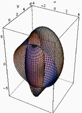
Figure 4: Fresnel wave surface for anisotropic permittivity $\varepsilon^{ab}=\hbox{diag}(39.7,15.4,2.3)$ and trivial impermeability $\mu^{-1}_{ab}=\mu_{0}^{-1}\hbox{diag}(1,1,1)$. The skewon field vanishes. There are two branches, the outer part of the surface is cut into half in order to show the inner branch. We use the dimensionless variables $x:=cq_{1}/q_{0},\,y:=cq_{2}/q_{0},\,z:=cq_{3}/q_{0}$.

Fresnel wave surfaces

Let us look at some Fresnel wave surfaces in order to get some feeling for the physics involved. Divide (53) by $q_{0}^{4}$ (here $q_{0}$ is the frequency of the wave) and introduce the dimensionless variables ($c$ = velocity of light in special relativity)

$$x_{a}:=c\,\frac{q_{a}}{q_{0}}\,.$$ (59)

Then we have

$$M+x_{a}\frac{M^{a}}{c}+x_{a}x_{b}\frac{M^{ab}}{c^{2}}+x_{a}x_{b}x_{c}\frac{M^{abc}}{c^{3}}+x_{a}x_{b}x_{c}x_{d}\frac{M^{abcd}}{c^{4}}=0\,.$$ (60)

We can draw these quartic surfaces in the dimensionless variables $x=x_{1}$, $y=x_{2}$, $z=x_{3}$, provided the $M$’s are given. According to (55)-(58), the $M$’s can be expressed in terms of the $3\times 3$ matrices $\mathfrak{A},\mathfrak{B},\mathfrak{C},\mathfrak{D}$. These matrices are specified in (38)-(40) in terms of the permittivity etc.. A comparison with the spacetime relations in the form of (41),(42) is particularly instructive.

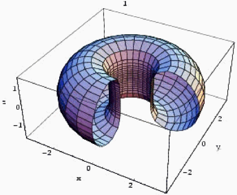
Figure 5: Fresnel wave surface for trivial permittivity $\varepsilon^{ab}=\varepsilon_{0}\,\hbox{diag}(1,1,1)$ and trivial impermeability $\mu^{-1}_{ab}=\mu_{0}^{-1}\hbox{diag}(1,1,1)$ with a skewon field of electric Faraday type ${\not\!S}_{3}{}^{0}=3.1\lambda_{0}$ (all other components vanish). The surface has the form of a toroid (depicted with two cuts). We use the dimensionless variables $x:=cq_{1}/q_{0},\,y:=cq_{2}/q_{0},\,z:=cq_{3}/q_{0}$.

Let us start with a simple example. We assume that the permittivity is anisotropic but still diagonal, $\varepsilon^{ab}=\hbox{diag}(\varepsilon_{1},\varepsilon_{2},\varepsilon_{3})$, whereas the impermeability is trivial $\mu^{-1}_{ab}=\mu_{0}^{-1}\hbox{diag}(1,1,1)$. No skewon field is assumed to exist. Whether an axion field is present or not doesn’t matter since the axion does not influence the light propagation in the geometrical optics limit. With Mathematica programs written by Tertychniy Sergey , we can construct for any values of $\varepsilon_{1},\varepsilon_{2},\varepsilon_{3}$ the Fresnel wave surface; an example is displayed in Fig.4.

More complicated cases are trivial permittivity $\varepsilon^{ab}=\varepsilon_{0}\,\hbox{diag}(1,1,1)$ and trivial impermeability $\mu^{-1}_{ab}=\mu_{0}^{-1}\hbox{diag}(1,1,1)$, but a nontrivial skewon field. We can take a skewon field of electric Faraday type ${\not\!S}_{3}{}^{0}$, for example, see Fig.5, or of magnetoelectric optical activity type ${\not\!S}_{1}{}^{2}={\not\!S}_{2}{}^{1}$, see Fig.6. In both figures and in the subsequent one $\lambda_{0}=\sqrt{\varepsilon_{0}/\mu_{0}}$ is the admittance of free space. The characteristic feature of the skewon field is the emergence of specific holes in the Fresnel surfaces that correspond to the directions in space along which the wave propagation is damped out completely skewon . This effect is in agreement with our earlier conclusion on the dissipative nature of the skewon field.

Figure 6: Fresnel wave surface for trivial permittivity $\varepsilon^{ab}=\varepsilon_{0}\,\hbox{diag}(1,1,1)$ and trivial impermeability $\mu^{-1}_{ab}=\mu_{0}^{-1}\hbox{diag}(1,1,1)$ with a skewon field of the magneto-electric optical activity type $\not\!S_{1}{}^{2}=\not\!S_{2}{}^{1}=0.8\,\lambda_{0}$ (all other components vanish). It has two intersecting toroidal branches. We use the dimensionless variables $x:=cq_{1}/q_{0},\,y:=cq_{2}/q_{0},\,z:=cq_{3}/q_{0}$.

Now we can combine anisotropic permittivity with the presence of a skewon field. Then we expect to find some kind of Fig.4 “enriched” with holes induced by the skewon field. This time we choose a spatially isotropic skewon field with $\not\!S_{1}{}^{1}=\not\!S_{2}{}^{2}=\not\!S_{3}{}^{3}=-\frac{1}{3}\not\!S_{0}{}^{0}\neq 0$. The outcome is depicted in Fig.7. The four holes confirm our expectation.

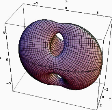
Figure 7: Fresnel wave surface for anisotropic permittivity $\varepsilon^{ab}=\hbox{diag}(2.4,14.8,54)$ and trivial impermeability $\mu^{-1}_{ab}=\mu_{0}^{-1}\hbox{diag}(1,1,1)$ with a spatially isotropic skewon field $\not\!S_{1}{}^{1}=\not\!S_{2}{}^{2}=\not\!S_{3}{}^{3}=-\frac{1}{3}\not\!S_{0}{}^{0}=0.25\,\lambda_{0}$ (all other components vanish). We use the dimensionless variables $x:=cq_{1}/q_{0},\,y:=cq_{2}/q_{0},\,z:=cq_{3}/q_{0}$.

11 No birefringence in vacuum and the light cone

The propagation of light in local and linear premetric vacuum electrodynamics is characterized by the extended Fresnel equation (52) or (54). We can solve the Fresnel equation with respect to the frequency $q_{0}$, keeping the 3–covector $q_{a}$ fixed. With the help of Mathematica, we found the following four solutions Laemmerzahl04 :

$$q_{0(\pm)}^{\uparrow} = \sqrt{\alpha}\pm\sqrt{\beta+\frac{\gamma}{\sqrt{\alpha}}}-\delta\,,$$ (61)

$$q_{0(\pm)}^{\downarrow} = -\sqrt{\alpha}\pm\sqrt{\beta-\frac{\gamma}{\sqrt{\alpha}}}-\delta\,.$$ (62)

We introduced the abbreviations

$$\alpha := \frac{1}{12M_{0}}\left(\frac{a}{\left(b+\sqrt{c}\right)^{\frac{1}{3}}}+\left(b+\sqrt{c}\right)^{\frac{1}{3}}-2M_{2}\right)+\delta^{2}\,,$$ (63)

$$\beta := \frac{1}{12M_{0}}\left(-\frac{a}{\left(b+\sqrt{c}\right)^{\frac{1}{3}}}-\left(b+\sqrt{c}\right)^{\frac{1}{3}}-4M_{2}\right)+2\delta^{2}\,,$$ (64)

$$\gamma := \frac{1}{4M_{0}}\left(2\delta M_{2}-M_{3}\right)-2\delta^{3}\,,\qquad\delta:=\frac{M_{1}}{4M_{0}}\,,$$ (65)

with

$$a := 12M_{0}M_{4}-3M_{1}M_{3}+M_{2}^{2}\,,$$ (66)

$$b := \frac{27}{2}M_{0}M_{3}^{2}-36M_{0}M_{2}M_{4}-\frac{9}{2}M_{1}M_{2}M_{3}+\frac{27}{2}M_{1}^{2}M_{4}+M_{2}^{3}\,,$$ (67)

$$c := {4}\left(b^{2}-a^{3}\right)\,.$$ (68)

Vanishing birefringence

Now, let us demand the absence of birefringence (also called double refraction). In technical terms this means, see the solutions (61), (62), that $\beta=0$ and $\gamma=0$. Then we have the degenerate solution

$$q_{0}^{\uparrow}=\sqrt{\alpha}-\frac{M_{1}}{4M_{0}}\,,\qquad q_{0}^{\downarrow}=-\sqrt{\alpha}-\frac{M_{1}}{4M_{0}}\,.$$ (69)

The condition $\gamma=0$ yields directly $M_{3}=M_{1}\left(4M_{0}M_{2}-M_{1}^{2}\right)/{8M_{0}^{2}}$, and, using this, we find

$$\alpha=\frac{3M_{1}^{2}-8M_{0}M_{2}}{16M_{0}^{2}}\,.$$ (70)

Thus,

$$q_{0}^{\uparrow\!\downarrow}=\pm\sqrt{\frac{3M_{1}^{2}-8M_{0}M_{2}}{16M_{0}^{2}}}-\frac{M_{1}}{4M_{0}}\,.$$ (71)

Accordingly, the quartic wave surface (54) in this case reduces to

$$[(q_{0}-q_{0}^{\uparrow})(q_{0}-q_{0}^{\downarrow})]^{2}=0\,.$$ (72)

Multiplication yields

$$q_{0}^{2}+\frac{1}{2}\,\frac{M_{1}}{M_{0}}\,q_{0}+\frac{1}{2}\,\frac{M_{2}}{M_{0}}-\frac{1}{8}\,\left(\frac{M_{1}}{M_{0}}\right)^{2}=0\,.$$ (73)

If we substitute $M_{0},M_{1},M_{2}$ as defined in (53), we have explicitly ($i,j=0,1,2,3$)

$$g^{ij}q_{i}q_{j}:=q_{0}^{2}+\frac{1}{2}\,\frac{M^{a}}{M}\,q_{0}q_{a}+\frac{1}{8}\left(4\,\frac{M^{ab}}{M}-\frac{M^{a}M^{b}}{M^{2}}\right)q_{a}q_{b}=0\,.$$ (74)

This equation is quadratic in the 4-dimensional wave covector $q_{i}$. Therefore we recover the conventional light cone of general relativity at each point of spacetime, see Fig. 8. Thereby the causal structure of spacetime is determined. Thus, up to a scalar factor, we derived the Riemannian metric of general relativity.

Moreover, as we have shown Birkbook ; Annals , we find the correct Lorentzian signature. The Lorentzian (also known as Minkowskian) signature can be traced back to the Lenz rule, which determines the sign of the $\dot{B}$ term in the induction law. And this sign is different from the one in the corresponding $\dot{\cal D}$ term in the Oersted-Ampère-Maxwell law. In other words, the Lorentz signature is encoded in the decomposition formulas (9) and (14). Neither is the minus sign in (9) a convention nor the plus sign of the $E\wedge d\sigma$ term in (14). Since the Lenz rule is related to the positivity of the electromagnetic energy, the same is true for the Lorentzian signature. This derivation of the signature of the metric of spacetime from electrodynamics provides new insight into the structures underlying special as well as general relativity.

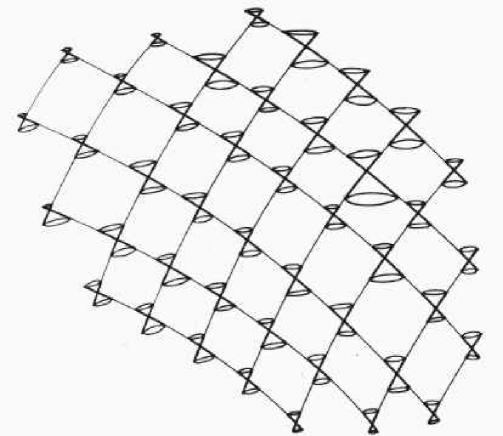
Figure 8: Null cones fitted together to form a conformal manifold (see Pirani and Schild Pirani ).

12 Dilaton, metric, axion

At first the skewon and the axion emerged at the premetric level in our theory and only subsequently the metric. Consequently, the axion and the skewon should be regarded as more fundamental fields (if they exist) than the metric. In the meantime, we phased out the skewon field since we insisted, in Sec.11, on vanishing birefringence in vacuum.

As to the metric, we recognize that multiplication of the metric by an arbitrary function $\tilde{\lambda}(x)$ was left open in the derivation of the last section, see (74):

$$\tilde{\lambda}(x)\,g^{ij}(x)\,q_{i}q_{j}=0\,.$$ (75)

Thus, only the conformally invariant part of the metric is determined. In other words, we have actually constructed the conformal (or the light cone) structure on the spacetime manifold, see, e.g., Weyl Weyl21 ; Weyl23 , Schouten Schouten54 , and Pirani & Schild Pirani .

It is known from special relativity that the light cone (with Lorentzian signature) is invariant under the 15-parameter conformal group, see Barut & Ra̧czka Barut and Blagojević Milutin . The latter, in Minkowskian coordinates $x^{i}$, is generated by the following four sets of spacetime transformations:

$${\rm Translations}\quad(4\ {\rm param.})\quad x^{i} \rightarrow\>\tilde{x}^{i}=\,x^{i}+a^{i}\,,$$ (76)

$${\rm Lorentz\ transf.}\quad(6\ {\rm param.})\quad x^{i} \rightarrow\>\tilde{x}^{i}=\,\Lambda^{i}{}_{j}\,x^{j}\,,$$ (77)

$${\rm dila(ta)tion}\quad(1\ {\rm param.})\quad x^{i} \rightarrow\>\tilde{x}^{i}=\,\rho\,x^{i}\,,$$ (78)

$${\rm prop.\ conf.\ transf.}\quad(4\ {\rm param.})\quad x^{i} \rightarrow\>\tilde{x}^{i}=\,{\frac{x^{i}+\kappa^{i}\,x^{2}}{1+2\kappa_{j}\,x^{j}+\kappa_{j}\kappa^{j}\,x^{2}}}.$$ (79)

Here $a^{i},\Lambda^{i}{}_{j},\rho,\kappa^{i}$ are the 15 constant parameters, and $x^{2}:=g_{ij}x^{i}x^{j}$. The Poincaré subgroup (76), (77) (for a modern presentation of it, see Giulini Giulini ) leaves the spacetime interval $ds^{2}=g_{ij}dx^{i}dx^{j}$ invariant, whereas the dilatations (78) and the proper conformal transformations (79) change the spacetime interval by a scaling factor $ds^{2}\rightarrow\rho^{2}ds^{2}$ and $ds^{2}\rightarrow\sigma^{2}ds^{2}$, respectively (with $\sigma^{-1}:=1+2\kappa_{j}\,x^{j}+\kappa_{j}\kappa^{j}\,x^{2}$). In all cases the light cone $ds^{2}=0$ is left invariant. The Weyl subgroup, which is generated by the transformations (76)-(78), and its corresponding Noether currents were discussed by, e.g., Kopczyński et al. Weylcurrents .

For massless particles, instead of the Poincaré group, the conformal or the Weyl group come under consideration, since massless particles move on the light cone. Even though the light cone stays invariant under all transformations (76)-(79), two reference frames that are linked to each other by a proper conformal transformation don’t stay inertial frames since their relative velocity is not constant. If one wants to uphold the inertial character of the reference frames, one has to turn to the Weyl transformation, that is, one has to specialize to $\kappa^{i}=0$.

The conformal group in Minkowski space illustrates the importance of the light cone structure on a flat manifold. This is suggestive for the light cone on an arbitrarily curved manifold, even though there is no direct relation between (76)-(79) and the light cone structure we derived in the last section.

The light cone metric $g^{ij}$ introduces the Hodge star ^⋆ operator. We then can straightforwardly verify that the principal part of the spacetime relation is determined as $H\sim{}^{\star}\!F$, where the coefficient of proportionality can be an arbitrary scalar function $\lambda(x)$ of the spacetime coordinates. This function is naturally identified with the dilaton field, see Brans Carl and Fujii & Maeda Fujii . Introducing the (Levi-Civita) dual of the excitation, $\check{H}^{ij}:=\frac{1}{2}\,\epsilon^{ijkl}\,H_{kl}$, we can then finally rewrite the spacetime relation for vanishing birefringence in vacuum as

$$\check{H}^{ij}=[\underbrace{\lambda(x)}_{\hbox{dilaton}}\!\!\sqrt{-g}\,g^{ik}(x)\,g^{jl}(x)+\underbrace{\alpha(x)}_{\hbox{axion}}\epsilon^{ijkl}\>]\,F_{kl}\,,$$ (80)

that is, we are left with the constitutive fields dilaton $\lambda$, metric $g^{ij}$, and axion $\alpha$. The combination $\sqrt{-g}\,g^{i[k}(x)\,g^{l]j}(x)$ is conformally invariant, in complete agreement with the above analysis.

13 Setting the scale

The conformal structure of spacetime is laid down in (74). Hence only 9 of the 10 independent components of the pseudo-Riemannian metric $g_{ij}$ are specified. We need, in addition to the conformal structure, a volume measure for arriving at a unique Riemannian metric. This can be achieved by postulating a time or length standard.

In exterior calculus, (80) reads

$${H=\lambda(x)\,^{\star}\!F+\alpha(x)\,F\,.}$$ (81)

The axion has not been found so far, so we can put $\alpha=0$. Moreover, under normal cicumstances, the dilaton seems to be a constant field and thereby sets a certain scale, i.e., $\lambda(x)=\lambda_{0}$, where $\lambda_{0}$ is the admittance of free space the value of which is, in SI-units, $1/(377\;\Omega)$. (The exact implementation of this assumption will have to be worked out in future.) Accordingly, we are left with the spacetime relation of conventional Maxwell-Lorentz electrodynamics

$$\boxed{H=\lambda_{0}\,^{\star}F}\qquad\hbox{or}\qquad\check{H}^{ij}=\lambda_{0}\sqrt{-g}\,g^{ik}(x)\,g^{jl}(x)\,F_{kl}=\lambda_{0}\sqrt{-g}\,F^{ij}\,.$$ (82)

14 Discussion

Weyl Weyl21 ; Weyl23 , in 1921, proved a theorem that the projective and the conformal structures of a metrical space determine its metric uniquely. As a consequence Weyl Weyl21 argued that …the metric of the world can be determined merely by observing the “natural” motion of material particles and the propagation of action, in particular that of light; measuring rods and clocks are not required for that. Here we find the two elementary notions for the determination of the metric: The paths of a freely falling point particles, yielding the projective structure, and light rays, yielding the conformal structure of spacetime. Later, in 1966, Pirani and Schild Pirani , amongst others, deepened the insight into the conformal structure and the Weyl tensor.

In 1972, on the basis of Weyl’s two primitive elements, Ehlers, Pirani, and Schild (EPS) EPS proposed an axiomatic framework in which Weyl’s concepts of free particles and of light rays were taken as elementary notions that are linked to each other by plausible axioms. Requiring compatibility between the emerging projective and conformal structures, they ended up with a Weyl spacetime(Riemannian metric with an additional Weyl covector). They set a scale [as we did in the last section, too] and arrived at the pseudo-Riemannian metric of general relativity. In this sense, EPS were able to reconstruct the metric of general relativity.

Subsequently, many authors improved and discussed the EPS-axiomatics. Access to the corresponding literature can be found via the book of Majer and Schmidt Majer or the work of Perlick Perlick91 ; Perlick00 and Lämmerzahl Lammerzahl01 , e.g.. For a general review one should compare Schelb Schelb and for a new axiomatic scheme Schröter Schroeter .

As stated, the point particles and light rays were primary elements that were assumed to exist and no link to mechanics nor to electrodynamics was specified. The particle concept within the EPS-axiomatics lost credibility when during the emergence of gauge theories of gravity (which started in 1956 with Utiyama Utiyama even before the EPS-framework had been set up in 1972) the first quantized wave function $\Psi$ for matter entered the scene as an elementary and “irreducible” concept in gravity theory. When neutron interference in an external gravitational field was discovered experimentally in 1975 by Collella, Overhauser, and Werner (COW) COW , see also RauchWerner , Sec.7, it was clear that the point particle concept in the EPS-framework became untenable from a physical point of view. For completeness let us mention some more recent experiments on matter waves in the gravitational field or in a noninertial frame:

• The Werner, Staudenmann, and Colella experiment Werner79 in 1979 on the phase shift of neutron waves induced by the rotation of the Earth (Sagnac-type effect),

• the Bonse & Wroblewski experiment Bonse84 in 1984 on neutron interferometry in a noninertial frame (verifying, together with the COW experiment, the equivalence principle for neutron waves),

• the Kasevich & Chu interferometric experiment Kasevich in 1991 with laser-cooled wave packets of sodium atoms in the gravitational field,

• the Mewes et al. experiment MewesKetterle in 1997 with interfering freely falling Bose-Einstein condensed sodium atoms, see Ketterle KetterleNobel , Fig.14 and the corresponding text,

• the Nesvizhevsky et al. experiment Nes1 ; Nes2 in 2002 on the quantum states of neutrons in the Earth’s gravitational field, and

• the Fray, Hänsch, et al. Fray experiment in 2004 with a matter wave interferometer based on the diffraction of atoms from effective absorption gratings of light. This interferometer was used for two stable isotopes of the rubidium atom in the gravitational field of the Earth. Thereby the equivalence principle was tested successfully on the atomic level.

Clearly, without the Schrödinger equation in an external gravitational field or in a noninertial frame all these experiments cannot be described. Still, in most textbooks on gravity, these experiments are not even mentioned!

In the 1980’s, as a reaction to the COW-experiment, Audretsch and Lämmerzahl, for a review see Audretsch , started to develop an axiomatic scheme for spacetime in which the point particle was substituted by a matter wave function and the light ray be a wave equation for electromagnetic disturbances. In this way, they could also include projective structures with an asymmetric connection (i.e., with torsion), which was excluded in the EPS approach a priori.

Turning to the conformal structure, which is in the center of our interest here, Lämmerzahl et al. JMP , see also Puntigam ; HauLaem , reconsidered the Audretsch-Lämmerzahl scheme and derived the inhomogeneous Maxwell equation from the following requirements: a well-posed Cauchy problem, the superposition principle, a finite propagation speed, and the absence of birefringence in vacuum. The homogeneous Maxwell equation they got by a suitable definition of the electromagnetic field strength. With a geometric optics approximation, compare our Sec.10, they recover the light ray in lowest order. And this is the message of this type of axiomatics: Within the axiomatic system of Audretsch and Lämmerzahl et al., the light ray, which is elementary in the EPS-approach, can be derived from reasonable axioms about the propagation of electromagnetic disturbances. As with the substitution of the mass point by a matter wave, this inquiry into the physical nature of the light ray and the corresponding reshaping of the EPS-scheme seems to lead to a better understanding of the metric of spacetime. And this is exactly where our framework fits in: We also build up the Maxwell equations in an axiomatic way and are even led to the signature of the metric, an achievement that needs still to be evaluated in all details.

15 Summary

Let us then summarize our findings: We outlined our axiomatic approach to electrodynamics and to the derivation of the light cone. In particular, with the help of a local and linear spacetime relation,

• we found the skewon field ${\not\!S}_{i}{}^{j}$ (15 components) and the axion field $\alpha$ (1 component),

• we found a quartic Fresnel wave surface for light propagation.

• In the case of vanishing birefringence, the Fresnel wave surface degenerates and we recovered the light cone (determining 9 components of the metric tensor) and, together with it, the conformal and causal structure of spacetime and the Hodge star ^⋆ operator.

• If additionally the dilaton $\lambda$ (1 component) is put to a constant, namely to the admittance of free space $\lambda_{0}$ [$1/(377\;\Omega)$ in SI-units], and the axion $\alpha$ removed, we recover the conventional Maxwell-Lorentz spacetime relation $H=\lambda_{0}\,^{\star}F$.

Thus, in our framework, the conformal part of the metric emerges from the local and linear spacetime relation as an electromagnetic construct. In this sense, the light cone is a derived concept.

References

- (1) J. Audretsch and C. Lämmerzahl, A new constructive axiomatic scheme for the geometry of space-time In Majer pp. 21–39 (1994).
- (2) A.O. Barut and R. Ra̧czka, Theory of Group Representations and Applications (PWN – Polish Scientific Publishers, Warsaw, 1977).
- (3) R. Beig, Concepts of Hyperbolicity and Relativistic Continuum Mechanics, arXiv.org/gr-qc/0411092.
- (4) M. Blagojević, Gravitation and Gauge Symmetries (IOP Publishing, Bristol, 2002).
- (5) U. Bonse and T. Wroblewski, Dynamical diffraction effects in noninertial neutron interferometry, Phys. Rev. D30 (1984) 1214–1217.
- (6) C.H. Brans, The roots of scalar-tensor theory: An approximate history, arXiv.org/gr-qc/0506063.
- (7) R. Colella, A.W. Overhauser, and S.A. Werner Observation of Gravitationally Induced Quantum Interference, Phys. Rev. Lett. 34 (1975) 1472–1474.
- (8) D.H. Delphenich, On the axioms of topological electromagnetism, Ann. Phys. (Leipzig) 14 (2005) 347–377; updated version of arXiv.org/hep-th/0311256.
- (9) D.H. Delphenich, Symmetries and pre-metric electromagnetism, Ann. Phys. (Leipzig) 14 (2005) issue 11 or 12, to be published.
- (10) I.E. Dzyaloshinskii, On the magneto-electrical effect in antiferromagnets, J. Exptl. Theoret. Phys. (USSR) 37 (1959) 881–882 [English transl.: Sov. Phys. JETP 10 (1960) 628–629].
- (11) D.G.B. Edelen, A metric free electrodynamics with electric and magnetic charges, Ann. Phys. (NY) 112 (1978) 366–400.
- (12) J. Ehlers, F.A.E. Pirani, and A. Schild, The geometry of free fall and light propagation, in: General Relativity, papers in honour of J.L. Synge, L. O’Raifeartaigh, ed. (Clarendon Press, Oxford, 1972), pp. 63–84.
- (13) A. Einstein, Zur Elektrodynamik bewegter Körper, Ann. Phys. (Leipzig) 17 (1905) 891–921. English translation in Dover1952 .
- (14) S. Fray, C. Alvarez Diez, T. W. Hänsch and M. Weitz, Atomic interferometer with amplitude gratings of light and its applications to atom based tests of the equivalence principle, Phys. Rev. Lett. 93 (2004) 240404 (4 pages); arXiv.org/physics/0411052.
- (15) C.D. Froggatt and H.B. Nielsen, Derivation of Poincaré invariance from general quantum field theory, Ann. Phys. (Leipzig) 14 (2005) 115–147 [Special issue commemorating Albert Einstein].
- (16) Y. Fujii and K.-I. Maeda, The Scalar-Tensor Theory of Gravitation (Cambridge University Press, Cambridge, 2003).
- (17) D. Giulini, The Poincaré group: Algebraic, representation-theoretic, and geometric aspects, these Proceedings (2005).
- (18) M. Haugan and C. Lämmerzahl, On the experimental foundations of the Maxwell equations, Ann. Phys. (Leipzig) 9 (2000) Special Issue, SI-119–SI-124.
- (19) F.W. Hehl and W.-T. Ni: Inertial effects of a Dirac particle. Phys. Rev. D42 (1990) 2045–2048.
- (20) F.W. Hehl and Yu.N. Obukhov, Foundations of Classical Electrodynamics — Charge, Flux, and Metric (Birkhäuser, Boston, MA, 2003).
- (21) F.W. Hehl and Yu.N. Obukhov, Electric/magnetic reciprocity in premetric electrodynamics with and without magnetic charge, and the complex electromagnetic field, Phys. Lett. A323 (2004) 169–175; arXiv.org/physics/0401083.
- (22) F.W. Hehl and Yu. N. Obukhov, Dimensions and units in electrodynamics, Gen. Rel. Grav. 37 (2005) 733–749; arXiv.org/physics/0407022.
- (23) F.W. Hehl and Yu.N. Obukhov, Linear media in classical electrodynamics and the Post constraint, Phys. Lett. A334 (2005) 249–259; arXiv.org/physics/ 0411038.
- (24) Y. Itin, Caroll-Field-Jackiw electrodynamics in the pre-metric framework, Phys. Rev. D70 (2004) 025012 (6 pages); arXiv/org/hep-th/0403023.
- (25) Y. Itin and F.W. Hehl, Is the Lorentz signature of the metric of spacetime electromagnetic in origin? Ann. Phys. (NY) 312 (2004) 60–83; arXiv.org/gr-qc/0401016.
- (26) G. Kaiser, Energy-momentum conservation in pre-metric electrodynamics with magnetic charges, J. Phys. A37 (2004) 7163–7168.
- (27) M. Kasevich and S. Chu, Atomic interferometry using stimulated Raman transitions, Phys. Rev. Lett. 67 (1991) 181–184.
- (28) W. Ketterle, When atoms behave as waves: Bose-Einstein condensation and the atom laser (Noble lecture 2001), http://nobelprize.org/physics/laureates/2001/ketterle-lecture.pdf .
- (29) R.M. Kiehn, Plasmas and Non Equilibrium Electrodynamics 2005 (312 pages), see http://www22.pair.com/csdc/download/plasmas85h.pdf .
- (30) W. Kopczyński, J.D. McCrea and F.W. Hehl, The Weyl group and its current. Phys. Lett. A128 (1988) 313–317.
- (31) C. Lämmerzahl, A characterisation of the Weylian structure of space-time by means of low velocity tests, Gen. Rel. Grav. 33 (2001) 815–831; arXiv.org/gr-qc/0103047.
- (32) C. Lämmerzahl, A. Camacho, and A. Macías, Reasons for the electromagnetic field to obey Maxwell’s equations, submitted to J. Math. Phys. (2005).
- (33) C. Lämmerzahl and F.W. Hehl, Riemannian light cone from vanishing birefringence in premetric vacuum electrodynamics, Phys. Rev. D70 (2004) 105022 (7 pages); arXiv.org/gr-qc/0409072.
- (34) C. Lämmerzahl, A. Macías, and H. Müller, Lorentz invariance violation and charge (non)conservation: A general theoretical frame for extensions of the Maxwell equations, Phys. Rev. D71 (2005) 025007 (15 pages).
- (35) I.V. Lindell, Differential Forms in Electromagnetics (IEEE Press, Piscataway, NJ, and Wiley-Interscience, 2004).
- (36) L.V. Lindell, The class of bi-anisotropic IB-media, J. Electromag. Waves Appl., to be published (2005).
- (37) I.V. Lindell and A.H. Sihvola, Perfect electromagnetic conductor, J. Electromag. Waves Appl. 19 (2005) 861–869; arXiv.org/physics/0503232.
- (38) I.V. Lindell, A.H. Sihvola, S.A. Tretyakov, A.J. Viitanen, Electromagnetic Waves in Chiral and Bi-Isotropic Media (Artech House, Boston, MA, 1994).
- (39) H.A. Lorentz, A. Einstein, H. Minkowski, and H. Weyl, The Principle of Relativity. A collection of original memoirs. Translation from the German (Dover, New York, 1952).
- (40) U. Majer and H.-J.Schmidt (eds.), Semantical Aspects of Spacetime Theories (BI-Wissenschaftsverlag, Mannheim 1994).
- (41) M.-O. Mewes et al., Output Coupler for Bose-Einstein Condensed Atoms, Phys. Rev. Lett. 78 (1997) 582–585.
- (42) V.V. Nesvizhevsky et al., Quantum states of neutrons in the Earth’s gravitational field, Nature 415 (2002) 297–299.
- (43) V.V. Nesvizhevsky et al., Measurement of quantum states of neutrons in the Earth’s gravitational field, Phys. Rev. D67 (2003) 102002 (9 pages); arXiv.org/hep-ph/0306198.
- (44) W.-T. Ni, Equivalence principles and precision experiments. In Precision Measurement and Fundamental Constants II, B.N. Taylor, W.D. Phillips, eds. Nat. Bur. Stand. (US) Spec. Publ. 617 (US Government Printing Office, Washington, DC, 1984) pp. 647–651.
- (45) Yu.N. Obukhov and F.W. Hehl, Possible skewon effects on light propagation, Phys. Rev. D70 (2004) 125015 (14 pages); arXiv.org/physics/0409155.
- (46) Yu.N. Obukhov and F.W. Hehl, Measuring a piecewise constant axion field in classical electrodynamics, Phys. Lett. A341 (2005) 357–365; arXiv.org/ physics/0504172.
- (47) V. Perlick, Observer fields in Weylian spacetime models, Class. Quantum Grav. 8 (1991) 1369–1385.
- (48) V. Perlick, Ray optics, Fermat’s principle, and applications to general relativity, Lecture Notes in Physics (Springer) m61 (2000) 220 pages.
- (49) F.A.E. Pirani and A. Schild, Conformal geometry and the interpretation of the Weyl tensor, in: Perspectives in Geometry and Relativity. Essays in honor of V. Hlavatý. B. Hoffmann, editor (Indiana University Press, Bloomington, 1966) pp. 291–309.
- (50) E.J. Post, Formal Structure of Electromagnetics – General Covariance and Electromagnetics (North Holland, Amsterdam, 1962, and Dover, Mineola, New York, 1997).
- (51) R.A. Puntigam, C. Lämmerzahl and F.W. Hehl, Maxwell’s theory on a post-Riemannian spacetime and the equivalence principle, Class. Quant. Grav. 14 (1997) 1347–1356; arXiv.org/gr-qc/9607023.
- (52) H. Rauch and S.A. Werner, Neutron Interferometry, Lessons in experimental quantum mechanics (Clarendon Press, Oxford, 2000).
- (53) G.F. Rubilar, Linear pre-metric electrodynamics and deduction of the lightcone, Thesis (University of Cologne, June 2002); see Ann. Phys. (Leipzig) 11 (2002) 717–782.
- (54) U. Schelb, Zur physikalischen Begründung der Raum-Zeit-Geometrie, Habilitation thesis (Univ. Paderborn, 1997).
- (55) J.A. Schouten, Ricci-Calculus, 2nd ed. (Springer, Berlin, 1954).
- (56) J. Schröter, A new formulation of general relativity. Part I. Pre-radar charts as generating functions for metric and velocity. Part II. Pre-radar charts as generating functions in arbitrary space-times. Part III. GTR as scalar field theory (altogether 58 pages). Preprint, Univ. Paderborn (July 2005).
- (57) B.D.H. Tellegen, The gyrator, a new electric network element, Philips Res. Rep. 3 (1948) 81–101.
- (58) B.D.H. Tellegen, The gyrator, an electric network element, in: Philips Technical Review 18 (1956/57) 120–124. Reprinted in H.B.G. Casimir and S. Gradstein (eds.) An Anthology of Philips Research. (Philips’ Gloeilampenfabrieken, Eindhoven, 1966) pp. 186–190.
- (59) S.I. Tertychniy [National Research Institute for Physical, Technical, and Radio-Technical Measurements (VNIIFTRI), 141570 Mendeleevo, Russia. Email: bpt97@mendeleevo.ru] provided the Mathematica programs for constructing the figures of the quartic Fresnel surface.
- (60) P. Teyssandier and R. W. Tucker, Gravity, Gauges and Clocks, Class. Quant. Grav. 13 (1996) 145–152.
- (61) R. Utiyama, Invariant theoretical interpretation of interaction, Phys. Rev. 101 (1956) 1597–1607.
- (62) S.A. Werner, J.-L. Staudenmann, and R. Colella, Effect of Earth’s rotation on the quantum mechanical phase of the neutron, Phys. Rev. Lett. 42 (1979) 1103–1106.
- (63) H. Weyl, Zur Infinitesimalgeometrie: Einordnung der projektiven und konformen Auffassung, Nachr. Königl. Gesellschaft Wiss. Göttingen, Math.-Phys. Klasse, pp. 99–112 (1921); also in K. Chandrasekharan (ed.), Hermann Weyl, Gesammelte Abhandlungen Vol.II, 195–207 (Springer, Berlin, 1968).
- (64) H. Weyl, Raum, Zeit, Materie, Vorlesungen über Allgemeine Relativitätstheorie, reprint of the 5th ed. of 1923 (Wissenschaftliche Buchges., Darmstadt, 1961). Engl. translation of the 4th ed.: Space–Time–Matter (Dover Publ., New York, 1952).
- (65) F. Wilczek, Two applications of axion electrodynamics, Phys. Rev. Lett. 58 (1987) 1799–1802.