The Renormalized Stress Tensor in Kerr Space-Time: Numerical Results for the Hartle-Hawking Vacuum

Abstract

We show that the pathology which afflicts the Hartle-Hawking vacuum on the Kerr black hole space-time can be regarded as due to rigid rotation of the state with the horizon in the sense that when the region outside the speed-of-light surface is removed by introducing a mirror, there is a state with the defining features of the Hartle-Hawking vacuum. In addition, we show that when the field is in this state, the expectation value of the energy-momentum stress tensor measured by an observer close to the horizon and rigidly rotating with it corresponds to that of a thermal distribution at the Hawking temperature rigidly rotating with the horizon.

I Introduction

We know that there is no Hadamard state on the Kerr black hole space-time with the defining features of the Hartle-Hawking vacuum of respecting the isometries of the space-time and being regular everywhere Kay and Wald (1991). Frolov and Thorne Frolov and Thorne (1989) have shown that with certain non-standard commutation relations a state can be found whose Feynman propagator formally has symmetry properties necessary for regularity of the state on the outer event horizon Hartle and Hawking (1976), however this state fails to be regular almost everywhere Ottewill and Winstanley (2000). The concensus in the literature is that the key property of the space-time which accounts for the non-existence of a true Hartle-Hawking vacuum is the presence of a region in which the Killing vector which is parallel to the null generators of the horizon becomes spacelike. In the present article we take up a suggestion made in Ref. Frolov and Thorne (1989) of removing this region from the space-time by enclosing the black hole within an axially symmetric, stationary mirror. We show that when this is done, there is a well behaved state with the defining features of the Hartle-Hawking vacuum. In addition, when the field is in this state the expectation value of the energy-momentum stress tensor as measured by an observer rigidly rotating with the horizon corresponds on the horizon to that of a thermal distribution at the Hawking temperature rigidly rotating with the horizon.

The mirror serves to remove the superradiant normal modes, as can be seen heuristically by noting that amplified waves which would otherwise escape to future null infinity are reflected by it across the future horizon. In the specific case of a mirror of constant Boyer-Lindquist radius, we can explicitly construct a vacuum state whose Feynman propagator has the symmetry properties identified in Ref. Hartle and Hawking (1976) and whose anticommutator function does not suffer from the pathology noted in Ref. Ottewill and Winstanley (2000). Although this conclusion appears to be valid irrespective of the radius of the mirror, we generalize a result due to Friedman Friedman (1978) to show that the space-time is unstable to scalar perturbations if the mirror does not remove all of the region outside the speed-of-light surface. This instability is characterized by the existence of mode solutions of the field equation with complex eigenfrequencies which we have neglected when quantizing the field. Kang Kang (1997) has shown that the contributions made by these modes to the response function of an Unruh box are not stationary but increase exponentially with time. We therefore believe that when part of the region lying outside the speed-of-light light surface is inside the mirror, it is not possible to construct the stationary states involved in our considerations.

The layout of the paper is as follows. In Sec. II we consider the normal mode solutions of the Klein-Gordon equation inside a mirror of constant Boyer-Lindquist radius. In Sec. III we use these solutions to numerically calculate the energy-momentum stress tensor as measured by observers rigidly rotating with the event horizon when the radius of the mirror is sufficiently small to remove all of the region outside the speed-of-light surface. In Sec. IV we consider the stability of the classical scalar field in the presence of a mirror and generalize Friedman’s result. Finally, in Sec. V we calculate numerically the eigenfrequencies of the unstable mode solutions of the field equation present when the black hole is inside a mirror of constant Boyer-Lindquist radius larger than the minimum radius of the speed-of-light surface. We follow the space-time conventions of Misner, Thorne and Wheeler Misner et al. (1973) and the notation of Ref. Ottewill and Winstanley (2000) throughout.

II Field in the Presence of a Mirror

We consider the right hand region of the Kerr black hole enclosed within a mirror $\mathcal{M}$ so that the past event horizon is a Cauchy surface for the space-time. We require that $\mathcal{M}$ respects the Killing isometries of the space-time since we are interested in a state which is invariant under these isometries. The simplest mirror is the hypersurface $r=r_{0}$ since the Klein-Gordon equation then still admits completely separable solutions. We take the radius of the mirror to be smaller than the minimum radius of the speed-of-light surface. We will see in Sec. IV that if the radius is larger, there are modes of complex frequency which need to be considered in addition to those discussed in this section. For brevity, we deal only with the case of a field satisfying Dirichlet conditions on this hypersurface.

We can construct normal modes by

$$s_{\omega lm}^{\mathrm{up}}(x)=\begin{cases}\displaystyle u_{\omega lm}^{\mathrm{up}}(x)-\frac{R_{\omega lm}^{\mathrm{up}}(r_{0})}{R_{\omega lm}^{\mathrm{in}}(r_{0})}u_{\omega lm}^{\mathrm{in}}(x),&\omega>0,\\ \displaystyle u_{\omega lm}^{\mathrm{up}}(x)-\frac{R_{\omega lm}^{\mathrm{up}}(r_{0})}{R_{-\omega l-m}^{\mathrm{in}*}(r_{0})}u_{-\omega l-m}^{\mathrm{in}*}(x),&\omega<0.\end{cases}$$ (1)

By convention, the ranges of our mode labels here and in what follows are appropriate to the “distant observer viewpoint” for modes with an ‘in’ or ‘out’ superscript and to the “near horizon viewpoint” for modes with an ‘up’ or ‘down’ superscript. The terminology here is that of Ref. Frolov and Thorne (1989). In the “distant observer viewpoint” $\omega\geq 0$ while in the “near horizon viewpoint” $\tilde{\omega}\geq 0$ where

$$\tilde{\omega}=\omega-m\Omega_{+}$$ (2)

and $\Omega_{+}$ is the angular velocity of the horizon with respect to static observers at infinity. It is straightforward to check that the modes $s_{\omega lm}^{\mathrm{up}}$ form an orthonormal set. If we let $h_{\omega lm}$ denote the solution of the radial equation which behaves like $e^{i\tilde{\omega}r_{*}}$ close to the horizon then the asymptotic form of $s_{\omega lm}^{\mathrm{up}}$ on the two horizons is

$$s_{\omega lm}^{\mathrm{up}}\sim\frac{S_{\omega lm}(\cos\theta)e^{im\varphi_{+}}}{\sqrt{8\pi^{2}\tilde{\omega}(r^{2}+a^{2})}}\begin{cases}e^{-i\tilde{\omega}u},&\mathcal{H}^{-},\\ \displaystyle-\frac{h_{\omega lm}(r_{0})}{h_{\omega lm}^{*}(r_{0})}e^{-i\tilde{\omega}v},&\mathcal{H}^{+}.\end{cases}$$ (3)

We see that, since $h_{\omega lm}(r_{0})/h_{\omega lm}^{*}(r_{0})$ is a complex constant with unit modulus, these modes are not superradiant.

We could equally well have constructed normal modes defined by

$$s_{\omega lm}^{\mathrm{down}}(x)=\begin{cases}\displaystyle u_{\omega lm}^{\mathrm{down}}(x)-\frac{R_{\omega lm}^{\mathrm{down}}(r_{0})}{R_{\omega lm}^{\mathrm{out}}(r_{0})}u_{\omega lm}^{\mathrm{out}}(x),&\omega>0,\\ \displaystyle u_{\omega lm}^{\mathrm{down}}(x)-\frac{R_{\omega lm}^{\mathrm{down}}(r_{0})}{R_{-\omega l-m}^{\mathrm{out}*}(r_{0})}u_{-\omega l-m}^{\mathrm{out}*}(x),&\omega<0,\end{cases}$$ (4)

which also satisfy the boundary conditions on the mirror and form an orthonormal set. It can be shown, however, that

$$s_{\omega lm}^{\mathrm{down}}(x)=-\frac{h_{\omega lm}^{*}(r_{0})}{h_{\omega lm}(r_{0})}s_{\omega lm}^{\mathrm{up}}(x),$$ (5)

and hence that these upgoing and downgoing modes differ from each other only by a phase. It follows that the vacuum state obtain by expanding the field in terms of either of these sets is the same and that this state is invariant under simultaneous $t$-$\varphi$ reversal. We denote it by $|B_{\mathcal{M}}\rangle$. Dropping the now superfluous superscript from the modes, the anticommutator function of $|B_{\mathcal{M}}\rangle$ is

$$G^{B_{\mathcal{M}}}_{\mathrm{(1)}}(x,x^{\prime})=\sum_{l=0}^{\infty}\sum_{m=-l}^{l}\int_{0}^{\infty}\mathrm{d}{\tilde{\omega}}\,\Re\left[s_{\omega lm}(x)s_{\omega lm}^{*}(x^{\prime})\right].$$ (6)

The modes with which the field has been expanded all have positive frequency with respect to the Killing vector $\boldsymbol{k}_{\mathcal{H}}$ given by

$$\boldsymbol{k}_{\mathcal{H}}=\boldsymbol{k}_{\mathcal{I}}+\Omega_{+}\boldsymbol{k}_{\circlearrowleft}.$$ (7)

Here, $\boldsymbol{k}_{\mathcal{I}}$ and $\boldsymbol{k}_{\circlearrowleft}$ are the two commuting Killing vectors of the Kerr space-time given in Boyer-Lindquist co-ordinates by

$$\boldsymbol{k}_{\mathcal{I}}=\partial_{t},\qquad\boldsymbol{k}_{\circlearrowleft}=\partial_{\varphi}.$$ (8)

It follows that an observer moving along an integral curve of $\boldsymbol{k}_{\mathcal{H}}$ makes measurements relative to the state $|B_{\mathcal{M}}\rangle$. Such an observer rotates rigidly with the same velocity as the horizon with respect to static observers at infinity. We call this observer a rigidly rotating observer (RRO).

We can extend $s_{\omega lm}$ to the left hand region of the space-time by requiring it to be zero there. If we place a similar mirror in this region then we can introduce a function $t_{\omega lm}$ defined by

$$t_{\omega lm}(U_{+},V_{+},\theta,\varphi_{+})=s_{\omega lm}^{*}(-U_{+},-V_{+},\theta,\varphi_{+}),$$ (9)

which has unit norm, satisfies the field equation, is zero in the right region of the space-time and satisfies the boundary condition on the mirror in the left hand region. Both of the linear combinations

$$\sigma_{\omega lm} =\frac{1}{\sqrt{1-e^{-2\pi\tilde{\omega}/\kappa_{+}}}}\left[s_{\omega lm}+e^{-\pi\tilde{\omega}/\kappa_{+}}t_{\omega lm}^{*}\right],$$ (10)

$$\tau_{\omega lm} =\frac{1}{\sqrt{1-e^{-2\pi\tilde{\omega}/\kappa_{+}}}}\left[t_{\omega lm}+e^{-\pi\tilde{\omega}/\kappa_{+}}s_{\omega lm}^{*}\right],$$ (11)

are regular functions of $U_{+}$ on the past event horizon which are analytic in the lower half of the complex $U_{+}$-plane and are regular functions of $V_{+}$ on the future event horizon which are analytic in the lower half of the complex $V_{+}$-plane. The vacuum state defined by expanding the field in terms of these is invariant under the simultaneous $t$-$\varphi$ reversal and has a Feynman propagator with the properties required of the Hartle-Hawking vacuum in Ref. Hartle and Hawking (1976). We denote this state by $|H_{\mathcal{M}}\rangle$. Its anticommutator function is

$$G^{H_{\mathcal{M}}}_{\mathrm{(1)}}(x,x^{\prime})=\sum_{l=0}^{\infty}\sum_{m=-l}^{l}\int_{0}^{\infty}\mathrm{d}{\tilde{\omega}}\,\coth\left(\frac{\pi\tilde{\omega}}{\kappa_{+}}\right)\Re\left[s_{\omega lm}(x)s_{\omega lm}^{*}(x^{\prime})\right].$$ (12)

III Numerical Results

The measurements of an RRO when the field is in the state $|H_{\mathcal{M}}\rangle$ can be calculated from

$$G^{H_{\mathcal{M}}}_{\mathrm{(1)}}(x,x^{\prime})-G^{B_{\mathcal{M}}}_{\mathrm{(1)}}(x,x^{\prime})=\sum_{l=0}^{\infty}\sum_{m=-l}^{l}\int_{0}^{\infty}\mathrm{d}{\tilde{\omega}}\,\frac{2}{e^{2\pi\tilde{\omega}/\kappa_{+}}-1}\Re\left[s_{\omega lm}(x)s_{\omega lm}^{*}(x^{\prime})\right].$$ (13)

The mode by mode cancellation of the high frequency divergences which afflict both anticommutator functions in the conincident limit makes this expression amenable to straightforward numerical analysis. We calculated the spheroidal functions and separation constants in essentially the same way as that outlined in Ref. Press et al. (1992). We calculated the radial functions by integrating Eq. (2.6) of Ref. Ottewill and Winstanley (2000). The accuracy of the integration has to be carefully considered in the case that $M\omega$ is small and $l$ is large. The details can be found in Ref. Duffy (2002) and will be outlined in a later article.

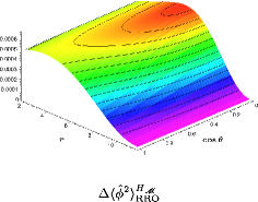
Figure 1: A graph of $\langle\hat{\phi^{2}}\rangle^{H_{\mathcal{M}}}_{\mathrm{RRO}}$, the expectation value of $\hat{\phi}^{2}$ measured by an RRO when the field is in the state $|H_{\mathcal{M}}\rangle$. The dark line gives the value on the horizon for a thermal distribution at the Hawking temperature rigidly rotating with the horizon. The units are such that $M=1$.

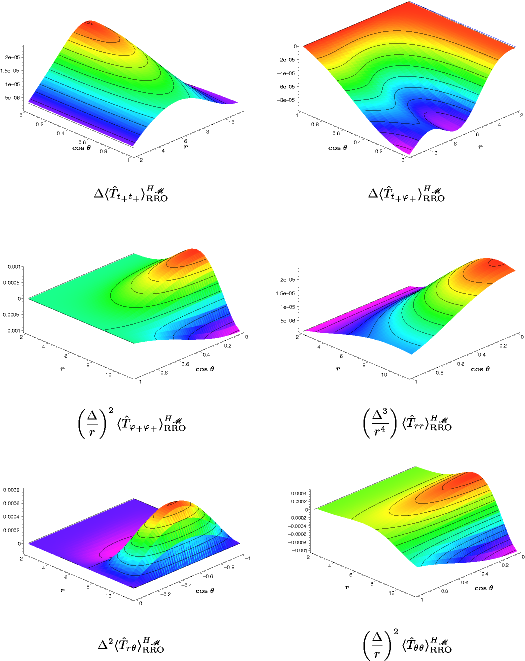
Figure 2: Graphs of the components of $\langle\hat{T}_{\mu\nu}\rangle^{H_{\mathcal{M}}}_{\mathrm{RRO}}$, the expectation value of the energy-momentum stress tensor measured by an RRO when the field is in the state $|H_{\mathcal{M}}\rangle$. The dark line gives the value on the horizon for a thermal distribution at the Hawking temperature rigidly rotating with the horizon. The units are such that $M=1$.

The graphs in Fig. 1 and Fig. 2 show the numerically calculated values of $\langle\hat{\phi^{2}}\rangle^{H_{\mathcal{M}}}_{\mathrm{RRO}}$ and $\langle\hat{T}_{\mu\nu}\rangle^{H_{\mathcal{M}}}_{\mathrm{RRO}}$, the expectation values measured by an RRO when the field is in the state $|H_{\mathcal{M}}\rangle$. They are given for a black hole for which $a=0.3M$ which means that $r_{+}=1.954M$. In all of the graphs, the units are such that $M=1$. The divergent behaviour as the horizon is approached has been factored out and each graph terminates on the mirror which has been given a radius $r_{0}=11.929M$. This is just smaller than the minimum radius of the speed-of-light surface, $r=11.935M$. See the appendix for the details of how this is calculated. On the horizon, the components are compared and show close agreement with those corresponding to a thermal distribution at the Hawking temperature rigidly rotating with the horizon. These are given by

$$\langle\phi^{2}\rangle^{T_{H}}_{\mathrm{}} =\frac{T^{2}}{12},$$ (14)

$$\langle T_{\mu\nu}\rangle^{T_{H}}_{\mathrm{}} =\frac{T^{4}\pi^{2}}{90}\left[g_{\mu\nu}-4\frac{k_{\mathcal{H}\mu}k_{\mathcal{H}\nu}}{k_{\mathcal{H}\sigma}k_{\mathcal{H}}^{\sigma}}\right],$$

where $T$ is the local temperature and is related to the Hawking temperature, $T_{H}$, by

$$T=\frac{T_{H}}{\sqrt{k_{\mathcal{H}\sigma}k_{\mathcal{H}}^{\sigma}}},\qquad T_{H}=\frac{\kappa_{+}}{2\pi}.$$ (15)

There has been some discussion in the literature about the rate of rotation of a Hartle-Hawking vacuum on the Kerr background, should it be possible to define such a state. It has been suggested, for example, that the state might appear isotropic to a ZAMO or an observer rotating at the angular rate of the Carter tetrad. The numerical calculations for the state $|H_{\mathcal{M}}\rangle$ provide strong evidence that it rotates rigidly up to not just leading order but also next to leading order as the horizon is approached. This is important because it shows that the rotation is not at the angular rate of either a ZAMO or the Carter tetrad. One way to see this is to consider an observer at fixed $r$ and $\theta$ rotating at an angular velocity of $\bar{\Omega}(r,\theta)$ relative to static observers at infinity. As an orthonormal tetrad carried by the observer we can take

$$\boldsymbol{e}_{(t)} =\frac{\gamma}{\alpha}\left[\partial_{t}+\bar{\Omega}\partial_{\varphi}\right],$$ (16)

$$\boldsymbol{e}_{(\varphi)} =\frac{1}{\gamma\tilde{\Omega}}\left[\partial_{\varphi}+\frac{\gamma^{2}\tilde{\Omega}^{2}}{\alpha^{2}}(\bar{\Omega}-\Omega)\left(\partial_{t}+\bar{\Omega}\partial_{\varphi}\right)\right],$$ (17)

$$\boldsymbol{e}_{(r)} =\sqrt{\frac{\Delta}{\Sigma}}\partial_{r},$$ (18)

$$\boldsymbol{e}_{(\theta)} =\sqrt{\frac{1}{\Sigma}}\partial_{\theta}.$$ (19)

We have introduced here standard functions of the metric components Misner et al. (1973)

$$\tilde{\Omega}=\sqrt{g_{\varphi\varphi}},\qquad\Omega=-\frac{g_{t\varphi}}{g_{\varphi\varphi}},\qquad\alpha=\sqrt{\frac{g_{t\varphi}^{2}-g_{tt}g_{\varphi\varphi}}{g_{\varphi\varphi}}}$$ (20)

and the function

$$\gamma=\sqrt{\frac{g_{t\varphi}^{2}-g_{tt}g_{\varphi\varphi}}{g_{\varphi\varphi}\left|g_{tt}+2\bar{\Omega}g_{t\varphi}+\bar{\Omega}^{2}g_{\varphi\varphi}\right|}}.$$ (21)

The function $\gamma$ is the Lorentz factor associated with the observer’s angular velocity relative to a ZAMO at the same point and $\Omega$ is the angular velocity of this ZAMO relative to static observers at infinity. Given an energy-momentum stress tensor $T_{\mu\nu}$, the flux of energy in the direction of $\boldsymbol{e}_{(\varphi)}$ measured by the observer is

$$T_{(t\varphi)} =\frac{1}{\alpha\tilde{\Omega}}\left[T_{t\varphi}+\bar{\Omega}T_{\varphi\varphi}+\frac{\gamma^{2}\tilde{\Omega}^{2}}{\alpha^{2}}(\bar{\Omega}-\Omega)(T_{tt}+2\bar{\Omega}T_{t\varphi}+\bar{\Omega}^{2}T_{\varphi\varphi})\right]$$ (22)

$$=\frac{\gamma^{2}\tilde{\Omega}}{\alpha^{3}}\left[\left(\frac{\alpha^{2}}{\tilde{\Omega}^{2}}+\Omega^{2}\right)T_{t\varphi}-\Omega T_{tt}+\bar{\Omega}\left(T_{tt}+\left(\frac{\alpha^{2}}{\tilde{\Omega}^{2}}+\Omega^{2}\right)T_{\varphi\varphi}\right)+\bar{\Omega}^{2}(T_{t\varphi}+\Omega T_{\varphi\varphi})\right]$$ (23)

The angular velocity at which the observer must rotate in order to measure no flux of energy is given by a root of the quadratic in $\bar{\Omega}$ appearing in the square brackets above. From the numerical data for $\langle\hat{T}_{\mu\nu}\rangle^{H_{\mathcal{M}}}_{\mathrm{RRO}}$, we can solve to find $\bar{\Omega}$. Fig. 3 gives a graph of $(\bar{\Omega}-\Omega_{+})/\Delta$. This is compared on the horizon with the value for an RRO, a ZAMO and an observer rotating with the same angular velocity as the Carter tetrad. These are given by

$$\lim_{r\to r_{+}}\left\{\frac{\bar{\Omega}-\Omega_{+}}{\Delta}\right\}=\begin{cases}0,&\bar{\Omega}=\Omega_{+},\\ -\frac{\Omega_{+}}{4M^{2}r_{+}\kappa_{+}},&\bar{\Omega}=\Omega_{\text{Carter}},\\ \Omega_{+}\left[\Omega_{+}^{2}\sin^{2}\theta+\frac{r_{-}}{4M^{2}r_{+}^{2}\kappa_{+}}\right],&\bar{\Omega}=\Omega.\end{cases}$$ (24)

The graph shows close agreement with the value corresponding to an RRO and not with either of the other two.

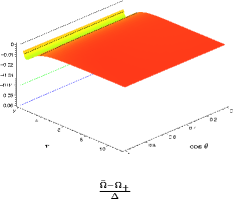
Figure 3: A graph of $(\bar{\Omega}-\Omega)/\Delta$, where $\bar{\Omega}$ is the rate of rotation of the frame in which there is no flux of energy. The black line gives the value on the horizon for $\bar{\Omega}=\Omega_{+}$, the blue line gives the value for $\bar{\Omega}=\Omega$ and the green line gives the value for $\bar{\Omega}=\Omega_{\text{Carter}}$.

It might be supposed that the behaviour of $\langle\hat{T}_{\mu\nu}\rangle^{H_{\mathcal{M}}}_{\mathrm{RRO}}$ close to the horizon is derivable by an asymptotic analysis in the manner of Candelas, Chrzanowski and Howard Candelas et al. (1981). Indeed, close to the horizon the contributions to the mode sums from the $u_{\omega lm}^{\mathrm{up}}$ dominate and we find that

$$\langle\hat{T}_{\mu\nu}\rangle^{H_{\mathcal{M}}}_{\mathrm{RRO}}\sim\langle CCH^{-}|\hat{T}_{\mu\nu}|CCH^{-}\rangle_{\mathrm{}}-\langle B^{-}|\hat{T}_{\mu\nu}|B^{-}\rangle_{\mathrm{}},\qquad(r\to r_{+}),$$ (25)

the right hand side of which has been calculated in Ref. Candelas et al. (1981) for the electromagnetic field. We wish to point out, however, that this analysis is unfortunately in error except at the poles of the horizon. The result given in Eq. (3.7) of Ref. Candelas et al. (1981) is obtained by noting that the dominant contributions come from the high $l$ modes and performing an asymptotic analysis of the ${}^{\vphantom{\mathrm{up}}}_{\pm 1}R_{\omega lm}^{\mathrm{up}}$ as the horizon is approached for large $l$. The spheroidal functions are also tacitly replaced with spherical functions. In general, however, contributions come from every value of $m$ and since the dominant contributions to the mode sum are for $\tilde{\omega}\approx T_{H}$, neither $\omega$ nor $m$ is necessarily small compared to $l$. The spheroidal functions therefore cannot always be approximated by spherical functions and the separation constant used in the analysis of the ${}^{\vphantom{\mathrm{up}}}_{\pm 1}R_{\omega lm}^{\mathrm{up}}$ cannot always be approximated by $l^{2}$. The poles are exceptional in that we know that only $m=\pm 1$ modes contribute there and that the analysis is therefore valid. This can be clearly seen from the result which can be written

$$\langle CCH^{-}|\hat{T}^{(\mu)}{}_{(\nu)}|CCH^{-}\rangle_{\mathrm{}}-\langle B^{-}|\hat{T}^{(\mu)}{}_{(\nu)}|B^{-}\rangle_{\mathrm{}}\sim\frac{11\pi^{2}T^{4}}{45}\left(\frac{\rho^{2}}{2Mr_{+}}\right)\mathop{\mathrm{diag}}(-3,1,1,1),\qquad(r\to r_{+}),$$ (26)

where the components are on the Carter tetrad. We have corrected here for a typographical error in Eq. (3.7) of Ref. Candelas et al. (1981) in which a factor of $r_{+}^{2}$ has been omitted. In Casals and Ottewill (2005) it was shown numerically that in fact

$$\langle CCH^{-}|\hat{T}^{(\mu)}{}_{(\nu)}|CCH^{-}\rangle_{\mathrm{}}-\langle B^{-}|\hat{T}^{(\mu)}{}_{(\nu)}|B^{-}\rangle_{\mathrm{}}\sim\frac{11\pi^{2}T^{4}}{45}\mathop{\mathrm{diag}}(-3,1,1,1),\qquad(r\to r_{+}),$$ (27)

which is precisely that of a thermal distribution at the Hawking temperature rigidly rotating with the horizon. These comments go equally well for the scalar field; following the method of Ref. Candelas et al. (1981) we would obtain values for $\langle\hat{\phi}^{2}\rangle^{H_{\mathcal{M}}}_{\mathrm{RRO}}$ and $\langle\hat{T}_{\mu\nu}\rangle^{H_{\mathcal{M}}}_{\mathrm{RRO}}$ incorrect by the same multiplicative factor of $\rho^{2}/(2Mr_{+})$.

The measurements of an RRO do not correspond to those of a thermal distribution everywhere. It is an open question whether or not their deviations from (14) are regular on the horizon. It can be checked by transforming to the Kruskal co-ordinate system that the conditions that $T_{\alpha\beta}$, given by

$$T_{\alpha\beta}=T^{\mathrm{th}}_{\alpha\beta}-\langle\hat{T}_{\alpha\beta}\rangle^{H_{\mathcal{M}}}_{\mathrm{RRO}},$$ (28)

is regular on both horizons are that at worst

$$T_{\varphi_{+}\varphi_{+}} =O(1), \quad T_{\theta\theta} =O(1), \quad T_{r\theta} =O(1),$$ (29)

$$T_{t_{+}t_{+}} =O(\Delta), \quad T_{t_{+}\varphi_{+}} =O(\Delta), \quad T_{t_{+}t_{+}}+\left(\frac{\Delta}{2Mr}\right)^{2}T_{rr} =O(\Delta^{2}).$$

These components are in the rigidly rotating co-ordinate system $\{t_{+},r,\theta,\varphi_{+}\}$ and we have placed a subscript on $t$ to avoid confusion with the Boyer-Lindquist co-ordinates. We have not been able to verify these numerically. It was conjectured by Christensen and Fulling Christensen and Fulling (1977) that for the Schwarzschild black hole, the measurements of a static observer when the field is in the Hartle-Hawking state would be exactly thermal everywhere. This was later shown not to be the case by Jensen, McLaughlin and Ottewill Jensen et al. (1992). Although the leading order of the deviation from isotropy is zero on the horizon in agreement with the asymptotic analyses of Christensen and Fulling (1977) and Candelas (1980), even in this case it remains undetermined whether or not the total deviation is regular there.

IV Stability of the Classical Scalar Field

The numerical calculations of the previous section fail if the radius of the mirror is increased to include any of the region in which $\boldsymbol{k}_{\mathcal{H}}$ becomes spacelike. If any of this region lies inside the mirror, new modes of the field equation come into existence which are also regular on the horizon and satisfy the boundary conditions on the mirror. These new modes have complex eigenfrequencies and are therefore characterized by the existence of unstable solutions of the field equation. We will show in this section that such solutions exist for all sufficiently high $m$. Kang Kang (1997) has demonstrated how to quantize the scalar field on the Kerr background in the presence of complex frequency modes. He has shown that the contributions made by them to the response function of an Unruh box are not stationary but increase exponentially with time and we expect that the anticommutator function will show similar behaviour. It follows that neither of the stationary states $|B_{\mathcal{M}}\rangle$ and $|H_{\mathcal{M}}\rangle$ exists unless the region outside the speed-of-light surface is removed by the mirror.

The analysis presented in this section is based heavily on that of Friedman Friedman (1978). The Lagrangian for the complex scalar field is

$$L=-\frac{1}{2}\int_{S_{t}}\boldsymbol{\eta}^{(3)}\alpha\nabla^{\mu}\phi\nabla_{\mu}\phi^{*},$$ (30)

where $S_{t}$ is a hypersurface of constant $t$, $\boldsymbol{\eta}^{(3)}$ is the volume $3$-form induced on $S_{t}$ by the metric and $\alpha$ is the lapse function given in Eq. (20) associated with the past pointing unit normal to $S_{t}$ which we denote by $\boldsymbol{n}$. The field equation is

$$\nabla^{\mu}\nabla_{\mu}\phi=0.$$ (31)

The total charge of the field at time $t$ is given by

$$\mathcal{Q}_{t}=i\int_{S_{t}}\boldsymbol{\eta}^{(3)}n^{\mu}\left[\phi^{*}\tensor{\nabla}_{\mu}\phi\right].$$ (32)

The total energy of the field at time $t$ depends on the Killing vector with which we define derivatives with respect to time. An appropriate vector is one of the form

$$\boldsymbol{k}=\boldsymbol{k}_{\mathcal{I}}+\Omega_{0}\boldsymbol{k}_{\circlearrowleft},\qquad\text{$\Omega_{0}$ constant,}$$ (33)

of which there is no preferred choice. The energy of the field on $S_{t}$ is

$$\mathcal{E}_{t}=\int_{S_{t}}\boldsymbol{\eta}^{(3)}n_{\mu}E^{\mu},$$ (34)

where

$$E^{\mu}=S^{\mu}{}_{\nu}k^{\nu},\quad S_{\mu\nu}=\nabla_{(\mu}\phi\nabla_{\nu)}\phi^{*}-\frac{1}{2}g_{\mu\nu}\nabla_{\sigma}\phi\nabla^{\sigma}\phi^{*}.$$ (35)

Consider the closed surface formed by the $S_{t}$, $S_{t^{\prime}}$ and the mirror as in Fig. 4.

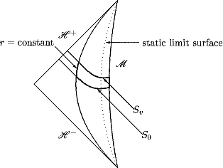
Figure 4: A space-time diagram of the region bounded by the surfaces $S_{t}$, $S_{t^{\prime}}$ and the mirror.

For a solution of the field equation, $\phi^{*}\tensor{\nabla}_{\mu}\phi$ is divergence free and so its flux over this surface is zero. Its flux over the mirror is zero by virtue of the boundary conditions and so its flux over $S_{t}$ is minus that over $S_{t^{\prime}}$. That is, $\mathcal{Q}_{t}$ is independent of $t$. These comments go equally well for $\boldsymbol{E}$ and so $\mathcal{E}_{t}$ is also independent of $t$.

Consider a solution of the field equation of the form

$$\phi_{\omega m}=\phi_{0}(r,\theta)e^{-i\omega t+im\varphi}.$$ (36)

Suppose that $\omega$ is complex so that the solution is unstable, growing exponentially either forwards or backwards in time. We find that

$$\mathcal{Q}_{t} =2e^{2\omega_{I}t}\int_{S_{t}}\boldsymbol{\eta}^{(3)}\frac{1}{\alpha}(\omega_{R}-m\Omega)|\phi_{0}|^{2},$$ (37)

$$\mathcal{E}_{t} =\frac{e^{2\omega_{I}t}}{2}\int_{S_{t}}\boldsymbol{\eta}^{(3)}\alpha\left\{g^{rr}\left|\frac{\partial\phi_{0}}{\partial r}\right|^{2}+g^{\theta\theta}\left|\frac{\partial\phi_{0}}{\partial\theta}\right|^{2}+\frac{1}{\alpha^{2}}\left[(\omega_{R}-m\Omega_{0})^{2}+\omega_{I}^{2}-m^{2}\frac{\boldsymbol{k}\cdot\boldsymbol{k}}{\tilde{\Omega}^{2}}\right]|\phi_{0}|^{2}\right\},$$ (38)

where

$$\omega_{R}=\Re[\omega],\qquad\omega_{I}=\Im[\omega].$$ (39)

We know that $\mathcal{Q}_{t}$ and $\mathcal{E}_{t}$ do not depend on $t$ and so it must be that the integrals in Eq. (37) and Eq. (38) vanish so that $\mathcal{Q}_{t}=0$ and $\mathcal{E}_{t}=0$. Thus, for an unstable mode

$$\int_{S_{t}}\boldsymbol{\eta}^{(3)}\frac{1}{\alpha}(\omega_{R}-m\Omega)|\phi_{0}|^{2} =0$$ (40)

$$\int_{S_{t}}\boldsymbol{\eta}^{(3)}\alpha\left\{g^{rr}\left|\frac{\partial\phi_{0}}{\partial r}\right|^{2}+g^{\theta\theta}\left|\frac{\partial\phi_{0}}{\partial\theta}\right|^{2}+\frac{1}{\alpha^{2}}\left[(\omega_{R}-m\Omega_{0})^{2}+\omega_{I}^{2}-m^{2}\frac{\boldsymbol{k}\cdot\boldsymbol{k}}{\tilde{\Omega}^{2}}\right]|\phi_{0}|^{2}\right\} =0.$$ (41)

Now if $\boldsymbol{k}$ can be chosen so that it remains timelike everywhere then it is clear that the integral on the left hand side of Eq. (41) must be positive for a non-trivial mode and so this condition cannot be met. There are therefore no unstable modes in this case. In particular, putting $\boldsymbol{k}=\boldsymbol{k}_{\mathcal{H}}$, we see that there are no unstable modes if the radius of the mirror is smaller than the minimum radius of the speed-of-light surface.

We could equally well have restricted the field to the region outside the mirror. This time putting $\boldsymbol{k}=\boldsymbol{k}_{\mathcal{I}}$, we see that there are no unstable modes if the radius of the mirror is larger than the maximum radius of the stationary limit surface. On the other hand, Friedman Friedman (1978) has shown that for a star with an ergoregion, unstable solutions to the Klein-Gordon equation exist. It can easily be checked that his analysis is valid for the Kerr space-time with the event horizon removed by surrounding the black hole with a mirror. We now show that there are likewise unstable solutions of the Klein-Gordon equation if we consider the space-time inside a mirror surrounding the black hole but not removing all of the region outside the speed-of-light surface.

Let $S_{v}$ be a family of hypersurfaces related to the Killing vector $\boldsymbol{k}_{\mathcal{H}}$ where the parameter $v$ satisfies $k^{\mu}_{\mathcal{H}}\nabla_{\mu}v=1$. The unit normal to each of these hypersurfaces is then given by

$$\boldsymbol{n}=-\alpha\,\mathrm{d}{v},\qquad\alpha=\frac{1}{\sqrt{-\nabla_{\mu}v\nabla^{\mu}v}}.$$ (42)

The vector $\boldsymbol{k}_{\mathcal{H}}$ can be decomposed into a part which is parallel and a part which is orthogonal to $\boldsymbol{n}$. That is,

$$\boldsymbol{\boldsymbol{k}_{\mathcal{H}}}=\alpha[\boldsymbol{n}+\beta\boldsymbol{m}],$$ (43)

where

$$m^{\mu}m_{\mu}=1,\quad n^{\mu}m_{\mu}=0.$$ (44)

The region inside the speed-of-light surface is clearly the region in which $|\beta|<1$. We can write the metric as

$$g_{\mu\nu}=-n_{\mu}n_{\nu}+m_{\mu}m_{\nu}+j_{\mu\nu},$$ (45)

where

$$\quad j^{\mu}{}_{\nu}=\delta^{\mu}{}_{\nu}+4n^{[\mu}m^{\sigma]}n_{[\nu}m_{\sigma]}.$$ (46)

The energy in the field on $S_{v}$ is

$$\mathcal{E}_{v}=\int_{S_{v}}\boldsymbol{\eta}^{(3)}n_{\mu}E^{\mu},$$ (47)

where $\boldsymbol{E}$ is defined in Eq. (35) with $\boldsymbol{k}=\boldsymbol{k}_{\mathcal{H}}$. Suppose that close to the future horizon the surfaces $S_{v}$ become null. Consider the region bounded by the surfaces $S_{0}$, $S_{v}$, a hypersurface of constant Boyer-Lindquist radius $r$ and the mirror as in Fig. 5.

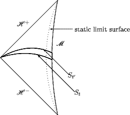
Figure 5: A space-time diagram of the region bounded by the surfaces $S_{0}$, $S_{v}$, a hypersurface of constant Boyer-Lindquist radius and the mirror.

Since the total flux of $\boldsymbol{E}$ over this surface is zero and its flux over the mirror is zero by virtue of the boundary conditions, we find that

$$\mathcal{E}_{v}=\mathcal{E}_{0}-2Mr_{+}\int_{0}^{v}\mathrm{d}{v}\int\mathrm{d}{\theta}\,\mathrm{d}{\varphi}\,\sin\theta\,\left|k^{\mu}_{\mathcal{H}}\nabla_{\mu}\phi\right|^{2},$$ (48)

In order to obtain the above expression we have taken the limit as the radius of the hypersurface of constant $r$ tends to the radius of the event horizon and used the condition that the field is regular on the horizon. This means that in the advanced co-ordinate system $\{\bar{t},r,\theta,\bar{\varphi}\}$ d’Inverno (1992), for example, $\phi$ can be expanded in $r$ about $r_{+}$ in terms of regular functions of $\bar{t}$, $\theta$ and $\bar{\varphi}$. Eq. (48) shows that a solution which is radiating energy across the future horizon looses energy between $S_{0}$ and $S_{v}$. To complete the proof we need to show that if $\boldsymbol{k_{\mathcal{H}}}$ becomes spacelike somewhere within the mirror then there is an initial configuration of the field for which $\mathcal{E}_{0}<0$. Then Eq. (48) implies that the field is at best marginally unstable and will be strictly unstable unless it can settle down at late $v$ to a non-radiative state. Furthermore, this non-radiative state state must be time-dependent. To see this note that from the field equation, $\mathcal{E}_{v}$ can be rewritten

$$\mathcal{E}_{v}=\frac{1}{2}\int_{S_{v}}\boldsymbol{\eta}^{(3)}n^{\mu}\Re\left[\left(k_{\mathcal{H}}^{\sigma}\nabla_{\sigma}\phi\right)\tensor{\nabla}_{\mu}\phi^{*}\right]$$ (49)

and hence is zero if $k^{\sigma}_{\mathcal{H}}\nabla_{\sigma}\phi$ is zero. We now show that there is an initial configuration of the field for which $\mathcal{E}<0$ if there is a region in which $\boldsymbol{k}_{\mathcal{H}}$ is spacelike. It is straightforward to show that the energy can be rewritten

$$\mathcal{E}_{0}=\frac{1}{2}\int_{S_{0}}\boldsymbol{\eta}^{(3)}\alpha\left[\left|n^{\mu}\nabla_{\mu}\phi\right|^{2}+2\beta\Re\left[\left(n^{\mu}\nabla_{\mu}\phi\right)\left(m^{\nu}\nabla_{\nu}\phi\right)\right]+\left|m^{\mu}\nabla_{\mu}\phi\right|^{2}+j^{\mu\nu}\nabla_{\mu}\phi\nabla_{\nu}\phi^{*}\right].$$ (50)

Suppose that in the region outside the speed-of-light surface, $S_{0}$ is a hypersurface of constant $t$. It then follows that

$$\boldsymbol{m}=\frac{\boldsymbol{k}_{\circlearrowleft}}{\tilde{\Omega}},\qquad\beta=\frac{\tilde{\Omega}}{\alpha}(\Omega_{+}-\Omega).$$ (51)

Let $O$ be an open region of $S_{0}$ lying outside the speed-of-light surface and let $O_{R}$ be an open ball of radius $R$ contained within $O$. Let $\varrho$ be a function which vanishes outside a compact subset of $O$, whose value and derivatives are bounded in such a way that there is a positive constant $K$ for which

$$\left|n^{\mu}\nabla_{\mu}\varrho\right|+\left|m^{\mu}\nabla_{\mu}\varrho\right|+\left|j^{\mu\nu}\nabla_{\mu}\varrho\nabla_{\nu}\varrho\right|^{1/2}<K,$$ (52)

and which on $O_{R}$ is given by

$$\varrho=1.$$ (53)

Consider the field which satisfies the initial conditions

$$\phi =\varrho e^{im\varphi_{+}},$$ (54)

$$n^{\mu}\nabla_{\mu}\phi =-m^{\mu}\nabla_{\mu}\phi.$$ (55)

This means that

$$\mathcal{E}_{0}=\frac{1}{2}\int_{S_{0}}\boldsymbol{\eta}^{(3)}\alpha\left[2(1-\beta)\left|m^{\mu}\nabla_{\mu}\phi\right|^{2}+j^{\mu\nu}\nabla_{\mu}\phi\nabla_{\nu}\phi^{*}\right]$$ (56)

There is an $\epsilon>0$ for which $1-\beta<-\epsilon$ everywhere within $O$. Suppose that within $O$, $\alpha$ is bounded between $\alpha_{\mathrm{min}}$ and $\alpha_{\mathrm{max}}$ and $\tilde{\Omega}$ is bounded above by $\tilde{\Omega}_{\mathrm{max}}$. It follows that

$$\mathcal{E}_{0} \leq-\epsilon\frac{\alpha_{\mathrm{min}}}{\tilde{\Omega}_{\mathrm{max}}^{2}}m^{2}\int_{O_{R}}\boldsymbol{\eta}^{(3)}+K^{2}\frac{\alpha_{\mathrm{max}}}{2}\int_{O}\boldsymbol{\eta}^{(3)}$$ (57)

$$=-\epsilon\frac{\alpha_{\mathrm{min}}}{\tilde{\Omega}_{\mathrm{max}}^{2}}m^{2}\left|O_{R}\right|+K^{2}\frac{\alpha_{\mathrm{max}}}{2}\left|O\right|,$$ (58)

where $|\cdot|$ indicates the $3$-volume. We see that $\mathcal{E}_{0}<0$ for all sufficiently high $m$.

V Numerical Search for Unstable Modes

Although we can say very little analytically about the occurence of complex frequency modes, we can obtain a bounded region of the complex plane within which the frequency must lie and thereby search for them numerically. From Eq. (40) we find that

$$0 \leq\omega_{R}\leq m\Omega_{+}, \qquad m >0,$$ (59)

$$0 \leq\tilde{\omega}_{R}\leq-m\Omega_{+}, \qquad m <0.$$ (60)

Using Eq. (40), we can write Eq. (41) as

$$\int_{S_{t}}\boldsymbol{\eta}^{(3)}\alpha\left\{g^{rr}\left|\frac{\partial\phi_{0}}{\partial r}\right|^{2}+g^{\theta\theta}\left|\frac{\partial\phi_{0}}{\partial\theta}\right|^{2}+\frac{1}{\alpha^{2}}\left[\omega_{I}^{2}-(\omega_{R}-m\Omega)^{2}+m^{2}\frac{\alpha^{2}}{\tilde{\Omega}^{2}}\right]|\phi_{0}|^{2}\right\}=0.$$ (61)

From the bound obtained for $\omega_{R}$, we find that

$$\omega_{I} \leq m\Omega_{+}, \qquad m >0,$$ (62)

$$\omega_{I} \leq-m\Omega_{+}, \qquad m <0.$$ (63)

Note from this that if a mode with complex frequency exists then the real part of its frequency is in the range which we associate with superradiance in the absence of a mirror. It is clear that there are no axially symmetric modes with complex frequency. It is also clear that when $a$ is set to zero and the space-time reduces to the Schwarzschild space-time, no such modes can occur as is well known. Curiously, the bound on the complex part of the frequency obtained in a similar analysis given by Detweiler and Ipser Detweiler and Ipser (1973) does not imply this.

Specializing to the case of a field satisfying Dirichlet conditions on the hypersurface $r=r_{0}$, we can now numerically search for complex frequency modes within this region. We look for a solution of the form

$$\phi=\frac{1}{\sqrt{r^{2}+a^{2}}}R_{\omega lm}(r)S_{\omega lm}(\cos\theta)e^{-i\omega t+im\varphi},$$ (64)

where

$$R_{\omega lm} \sim e^{-i\tilde{\omega}r_{*}}, (r_{*}\to-\infty),$$ (65)

$$R_{\omega lm} =0, r=r_{0}.$$ (66)

This can be cast as a root-finding problem for a complex function of a complex variable. The variable is $\omega$ and the function is $R_{\omega lm}(r_{0})$, obtained by integrating the radial differential equation from the horizon subject to the condition (65). Close to the horizon, $R_{\omega lm}$ increases exponentially with increasing $r_{*}$ and so there are no numerical problems in maintaining the accuracy of the integration. It is necessary to know the separation constant $\lambda_{\omega lm}$ and we have calculated this by using a power series expansion in $a\omega$ Abramowitz and Stegun (1964). The root-finding algorithm we have used is an iterative scheme known as Muller’s method Press et al. (1992).

Fig. 6 shows some of the results. We fix the value of $a$ and track the movement of the frequencies found as the value of $r_{0}$ changes. As the radius of the mirror decreases, the frequencies approach the real axis and pass into the lower half of the complex plane before the radius of the mirror reaches the minimum radius of the speed-of-light surface. In each case, the point at which they cross the real axis is the critical frequency of superradiant scattering in the absence of a mirror, $\tilde{\omega}=0$. This is expected in the case that the speed-of-light surface and the static limit surface do not cross. The reason for this is that if $\omega$ is real then $\phi$ satisfies the conditions to be an ingoing function. That is,

$$\phi=u_{\omega lm}^{\mathrm{in}},$$ (67)

when suitably normalized. Since $\phi^{*}$ also vanishes on the mirror, it is clear that the corresponding upgoing function, $u_{\omega lm}^{\mathrm{up}}$ does also. It is straightforward to check that $u_{\omega lm}^{\mathrm{up}}$ is an unstable mode in the field theory outside the mirror. However, we know from Friedman (1978) that there are no non-trivial modes of this type if the mirror lies entirely outside the stationary limit surface. The graphs in Fig. 6 show that this behaviour of the complex frequencies also occurs when the black hole is rotating sufficiently quickly that the speed-of-light surface lies partly within the static limit surface and the argument given above fails. The graphs are for the case $a=0.95M$, for which the relevant surfaces are shown in Fig. 7.

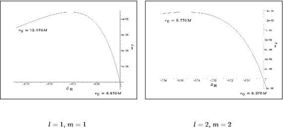
Figure 6: A graph of the complex eigenfrequencies corresponding to solutions of the Klein-Gordon equation which are null in the field theory inside a mirror of constant Boyer-Lindquist radius $r_{0}$ for a black hole with $a=0.95M$. As $r_{0}$ decreases, the frequencies pass into the lower complex plane through the point $\tilde{\omega}=0$ before the minimum radius of the speed-of-light surface, $r_{\mathrm{SOL}}(\pi/2)=1.675855M$, is reached. The eigenfrequency is given in units in which $M=1$.

VI Conclusions

In this paper, we investigated the pathology which afflicts the Hartle-Hawking vacuum on the Kerr black hole space-time. We have done this by taking up a suggestion made in Ref. Frolov and Thorne (1989) of enclosing the black hole within a mirror. The mirror serves to modify the global properties of the space-time without altering its differential geometry. We have found that the pathology can be regarded as due to rigid rotation of the state with the horizon in the sense that (1) when the mirror removes the region outside the speed-of-light surface, there is a state with the defining features of the Hartle-Hawking vacuum; (2) when the field is in this state, the expectation value of the energy-momentum stress tensor measured by an observer close to the horizon and rigidly rotating with it corresponds to that of a thermal distribution at the Hawking temperature rigidly rotating with the horizon; (3) when the mirror encloses any part of the region outside the speed-of-light surface, the field equation admits unstable solutions and it is not possible to construct any stationary state such as the Hartle-Hawking vacuum. We performed the calculation of the energy-momentum stress tensor by numerically solving for the mode solutions of the field equation and performing mode sums. In a future article, we will present a more detailed description of some of the numerical techniques used. We will also give there results for the Unruh vacuum.

*

Appendix

The speed-of-light surface is the hypersurface other than the horizon on which $\boldsymbol{k}_{\mathcal{H}}$ becomes null. In Boyer-Lindquist co-ordinates this is given by the condition

$$g_{tt}+2\Omega_{+}g_{t\varphi}+\Omega_{+}^{2}g_{\varphi\varphi}=0.$$ (68)

In terms of $r$ and $\theta$ this can be rewritten as

$$\frac{\Omega_{+}^{2}\sin^{2}\theta}{\Sigma}(r-r_{+})(r^{3}+Ar^{2}+Br+C)=0,$$ (69)

where

$$A =r_{+},$$ (70)

$$B =a^{2}\cos^{2}\theta+2Mr_{+}\left(1-\frac{2Mr_{+}}{a^{2}\sin^{2}\theta}\right),$$ (71)

$$C =(r_{+}-2M)\left(a^{2}\cos^{2}\theta-\frac{4M^{2}r_{+}^{2}}{a^{2}\sin^{2}\theta}\right)-4M^{2}r_{+}.$$ (72)

The cubic polynomial in $r$ which appears as a factor has only one real root $r_{\mathrm{SOL}}$ which we can solve for in terms of $\theta$ Spiegel (1968),

$$r_{\mathrm{SOL}}(\theta)=2\sqrt{-Q}\cos\left(\frac{\Theta}{3}\right)-\frac{A}{3}$$ (73)

where

$$Q=\frac{3B-A^{2}}{9},\quad P=\frac{9AB-27C-2A^{3}}{54},\quad\Theta=\cos^{-1}\left(\frac{P}{\sqrt{-Q^{3}}}\right).$$ (74)

It can be checked that $r_{\mathrm{SOL}}$ has a minimum value in the equatorial plane and that this is given by

$$r_{\mathrm{SOL}}\left(\frac{\pi}{2}\right)=\frac{r_{+}}{2}\left(\sqrt{1+\frac{8Mr_{+}}{a^{2}}}-1\right).$$ (75)

For a black hole with $a=0.3M$, which is considered above, the minimum radius of the speed-of-light surface is $r=11.935M$. As can bee seen, it is possible for the speed-of-light surface to lie partly within the static limit surface. When $a=\sqrt{2(\sqrt{2}-1)}M$ the two surfaces just touch in the equatorial plane and in the case of an extremal black hole, $a=M$, the speed-of-light surface just touches the outer horizon in the equatorial plane.

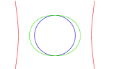
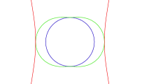
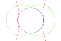
Figure 7: Schematic diagrams of the horizon (blue line), static limit surface (green line) and speed-of-light surface (red line) for $a=0.5M$, $a=\sqrt{2(\sqrt{2}-1)}M$ and $a=0.95M$. The diagrams show a $t=\text{constant}$, $\varphi=\text{constant}$ slice with the Boyer-Lindquist co-ordinates $r$ and $\theta$ used as plane polar co-ordinate.