Probing anisotropies of gravitational-wave backgrounds
with a space-based interferometer II:
perturbative reconstruction of a low-frequency skymap

Abstract

We present a perturbative reconstruction method to make a skymap of gravitational-wave backgrounds (GWBs) observed via space-based interferometer. In the presence of anisotropies in GWBs, the cross-correlated signals of observed GWBs are inherently time-dependent due to the non-stationarity of the gravitational-wave detector. Since the cross-correlated signal is obtained through an all-sky integral of primary signals convolving with the antenna pattern function of gravitational-wave detectors, the non-stationarity of cross-correlated signals, together with full knowledge of antenna pattern functions, can be used to reconstruct an intensity map of the GWBs. Here, we give two simple methods to reconstruct a skymap of GWBs based on the perturbative expansion in low-frequency regime. The first one is based on harmonic-Fourier representation of data streams and the second is based on “direct” time-series data. The latter method enables us to create a skymap in a direct manner. The reconstruction technique is demonstrated for the case of the Galactic gravitational wave background observed via planned space interferometer, LISA. Although the angular resolution of low-frequency skymap is rather restricted, the methodology presented here would be helpful in discriminating the GWBs of galactic origins by those of the extragalactic and/or cosmological origins.

I Introduction

The gravitational-wave background, incoherent superposition of gravitational waves coming from many unresolved point-sources and/or diffuse-sources would be a cosmological gold mine to probe the dark side of the Universe. While these signals are generally random and act as confusion noises with respect to a periodic gravitational-wave signal, the statistical properties of gravitational-wave backgrounds (GWBs) carry valuable information such as physical processes of gravitational-wave emission, source distribution and populations. Moreover, the extremely early universe beyond the last-scattering surface of cosmic microwave background (CMB) can be directly explored using GWB. Therefore, GWBs may be regarded as an ultimate cosmological tool alternative to the CMB.

Currently, several grand-based gravitational-wave detectors are now under scientific operation, and the search for gravitational waves enters a new era. There are several kinds of target GW sources in these detectors, such as, coalescence of neutron star binaries and core-collapsed supernova. On the other hand, planned space-based detector, LISA (Laser Interferometer Space Antenna) and the next-generation detectors, e.g., DECIGO Seto et al. (2001) and BBO BBO (2003) aim at detecting gravitational waves in low-frequency band $0.1$mHz –$0.1$Hz, in which many detectable candidates for GWBs exist. Among them, the GWB originated from the inflationary epoch may be detected directly in this band (e.g., Ungarelli and Vecchio (2001a); Smith et al. (2005)). Therefore, for future application to cosmology, various implications for these GWBs should deserve consideration both from the theoretical and the observational viewpoint.

One fundamental issue to access a new subject of cosmology is to make a skymap of GWB as a first step. Similar to the case of the CMB, the intensity map of the GWBs is of particular interest and it provides valuable information, which plays a key role to clarify the origin of GWBs. Importantly, the low-frequency GWBs observed by LISA are expected to be anisotropic due to the contribution of Galactic binaries to the confusion noise (Hils et al. (1990); Bender and Hils (1997); Nelemans et al. (2001), see also recent numerical simulations Benacquista et al. (2004); Edlund et al. (2005); Timpano et al. (2005)). Thus, the GWB skymap is potentially useful to discriminate the individual backgrounds from many superposed GWBs, as well as to identify the underlying physical processes. The basic idea to create a skymap of GWB is to use the directional information obtained through the time-modulation of the correlation signals, which is caused by the motion of gravitational-wave detector. As detector’s antenna pattern sweeps out the sky, the amplitude of the gravitational-wave signal would gradually change in time if the intensity distribution of GWB is anisotropic. Using this, a method to explore anisotropies of GWB has been proposed Giampieri and Polnarev (1997a, b); Allen and Ottewill (1997). Later, the methodology was applied to study the anisotropic GWB observed by space interferometer, LISA Ungarelli and Vecchio (2001b); Cornish (2001, 2002a); Seto (2004); Seto and Cooray (2004).

In the previous paper Kudoh and Taruya (2005a), which is referred to as Paper I in the present paper, we have investigated the directional sensitivity of space interferometer to the anisotropy of GWB. Particularly focusing on the geometric properties of antenna pattern functions and their angular power, we found that the angular sensitivity to the anisotropic GWBs is severely restricted by the data combination and the symmetry of detector configuration. As a result, in the case of the single LISA detector, detectable multipole moments are limited to $\ell\lesssim 8$–$10$ with the effective strain sensitivity $h\sim 10^{-20}$ Hz^-1/2. This is marked contrast to the angular sensitivity to the chirp signals emitted from point sources, in which the angular resolution can reach at a level of a square degree or even better than that Cutler (1998); Moore and Hellings (2002); Peterseim et al. (1997); Takahashi and Nakamura (2003).

Despite the poor resolution of LISA detector with respect to GWBs, making a skymap of GWBs is still an important general issue and thus needs to be investigated. In the present paper, we continue to investigate the map-making problem and consider how the intensity map of the GWBs is reconstructed from the time-modulation signals observed via space interferometer. In particular, we are interested in the low-frequency GWB, the wavelength of which is longer than the arm-length of the detector. In such case, the frequency dependence of the detector response becomes simpler and a perturbative scheme based on the low-frequency expansion of the antenna pattern functions can be applied. Owing to the least-squares approximation, we present a robust reconstruction method. The methodology is quite general and is also applicable to the map-making problem in the case of the ground detectors. We demonstrate how the present reconstruction method works well in a specific example of GWB source, i.e., Galactic confusion-noise background. With a sufficient high signal-to-noise ratio for each anisotropic components of GWB, we show that the space interferometer LISA can create the low-frequency skymap of Galactic GWB with angular resolution $\ell\leq 5$. Since the resultant skymap is obtained in a non-parametric way without any assumption of source distributions, we hope that despite the poor angular resolution, the present methodology will be helpful to give a tight constraint on the luminosity distribution of GWBs if we combine it with the other observational techniques.

The organization of the paper is as follows. In Sec. II, a brief discussion on the detection and the signal processing of anisotropic GWBs is presented, together with the detector response of space interferometer. Sec.III describes the details of the reconstruction of a GWB skymap in low-frequency regime. Owing to the least-squares approximation and the low-frequency expansion, a perturbative reconstruction scheme is developed. Related to this (in the case of LISA), and we give an important remark on the degeneracy between some multipole moments (Appendix B). In Sec.IV, the reconstruction method is demonstrated in the case of the Galactic GWB. The signal-to-noise ratios for anisotropy of GWB are evaluated and the feasibility to make a skymap of GWB is discussed. Finally, Section V is devoted to a summary and conclusion.

II Basic formalism

II.1 Correlation analysis

Let us begin with briefly reviewing the signal processing of gravitational-wave backgrounds based on the correlation analysis Kudoh and Taruya (2005a). Stochastic gravitational-wave backgrounds are described by incoherent superposition of plane gravitational waves ${\mathbf{h}}=h_{ij}$ given by

$${\mathbf{h}}(t,\mathbf{x})=\sum_{A=+,\times}\int_{-\infty}^{+\infty}df\int d\mathbf{\Omega}\,\,e^{i\,\,2\pi\,f(t-\mathbf{\Omega}\cdot\mathbf{x})}\,\tilde{h}_{A}(f,\mathbf{\Omega})\,\mathbf{e}^{A}(\mathbf{\Omega}).$$ (1)

The Fourier amplitude $\tilde{h}_{A}(f,\mathbf{\Omega})$ of the gravitational waves for the two polarization modes ${\mathbf{e}}^{A}$ ($A=+,\times$) is assumed to be characterized by a stationary random process with zero mean $\big{\langle}\widetilde{h}_{A}\big{\rangle}=0$. The power spectral density $S_{h}$ is then defined by

$$\left\langle\widetilde{h}_{A}^{*}(f,{\bf{\Omega}}){{\widetilde{h}}_{A^{\prime}}}(f^{\prime},{\bf{\Omega}}^{\prime})\right\rangle = \frac{1}{2}\delta(f-f^{\prime})\frac{\delta^{2}({\bf{\Omega}}-{\bf{\Omega}}^{\prime})}{4\pi}\delta_{AA^{\prime}}S_{h}(|f|,\,\mathbf{\Omega}),$$ (2)

where ${\mathbf{\Omega}}$ is the direction of a propagating plane wave. Note that the statistical independence between two different directions in the sky is implicitly assumed in equation (2), which might not be generally correct. Actually, CMB skymap exhibits a large-angle correlation between the different skies, which reflects the primordial density fluctuations. For the GWB of our interest, the wavelength of the tensor fluctuations detected via space interferometers is much shorter than the cosmological scales and thereby the assumption put in equation (2) is practically valid.

The detection of a gravitational-wave background is achieved through the correlation analysis of two data streams. The planned space interferometer, LISA and also the next generation detectors DECIGO/BBO constitute several spacecrafts, each of which exchanges laser beams with the others. Combining these laser pulses, it is possible to synthesize the various output streams which are sensitive (or insensitive) to the gravitational-wave signal. The output stream for a specific combination $I$ denoted by $s_{I}(t)$ is generally described by a sum of the gravitational-wave signal $h_{I}(t)$ and the instrumental noise $n_{I}(t)$ by

$$s_{I}(t)=h_{I}(t)+n_{I}(t).$$

We assume that the noise $n_{I}(t)$ is treated as a Gaussian random process with spectral density $S_{\rm n}(f)$ and zero mean $\big{\langle}n_{I}\big{\rangle}=0$. The gravitational-wave signal $h_{I}$ is obtained by contracting $\mathbf{h}$ with detector’s response function and/or detector tensor ${\mathbf{D}}:=D_{ij}$:

$$h_{I}(t)=\sum_{A=+,\times}\int_{-\infty}^{+\infty}df\int d\mathbf{\Omega}~{}e^{i2\pi f(t-\mathbf{\Omega}\cdot\mathbf{x}_{I})}{\textbf{D}}_{I}({\mathbf{\Omega}},f;t)\,{\textbf{:}}\,\mathbf{e}^{A}(\mathbf{\Omega})\,\,\widetilde{h}_{A}(f,\mathbf{\Omega}).$$ (3)

Note that the response function explicitly depends on time. The time variation of response function is caused by the orbital motion of the detector and it plays a key role in reconstructing a skymap of the GWBs. Typically, the orbital frequency of the detector motion is much lower than the observed frequency and within the case, the expression (3) is validated.

Provided the two output data sets, the correlation analysis is examined depending on the strategy of data analysis, i.e., self-correlation analysis using the single data stream or cross-correlation analysis using the two independent data stream. Defining $S_{IJ}(t)\equiv\left\langle s_{I}(t)s_{J}(t)\right\rangle$, the Fourier counterpart of it $\widetilde{S}_{IJ}(t,f)$, which is related with $S_{IJ}(t)$ by $S_{IJ}(t)=\int df\widetilde{S}_{IJ}(t,f)$, becomes

$$\widetilde{S}_{IJ}(t,f) = \widetilde{C}_{IJ}(t,f)+\delta_{IJ}\,\,S_{n}(|f|),$$ (4)

where we define

$$\widetilde{C}_{IJ}(t,f)=\int\frac{d\mathbf{\Omega}}{4\pi}S_{h}(|f|,\mathbf{\Omega})~{}\mathcal{F}_{IJ}^{E}(f,\mathbf{\Omega};\,t).$$ (5)

Here, the function $\mathcal{F}^{E}_{IJ}$ is the so-called antenna pattern function defined in an ecliptic coordinate, which is expressed in terms of detector’s response function:

$$\mathcal{F}^{E}_{IJ}(f,\mathbf{\Omega};\,t)=e^{i\,2\pi f\,{\bf\Omega\cdot}(\textbf{x}_{I}-\textbf{x}_{J})}\sum_{A=+,\times}F_{I}^{A*}(\mathbf{\Omega},f;\,t)F_{J}^{A}(\mathbf{\Omega},f;\,t)$$ (6)

$$F_{I}^{A}(\mathbf{\Omega},f;\,t)={\bf D}_{I}(\mathbf{\Omega},f;\,t)\,\textbf{:}\,\textbf{e}^{A}(\mathbf{\Omega})$$ (7)

Apart from the second term, equation (4) implies that the luminosity distribution of GWBs $S_{h}(f,\mathbf{\Omega})$ can be obtained by deconvolving the all-sky integral of antenna pattern function from the time-series data $S_{IJ}(t)$. To see this more explicitly, we focus on equation (5) and decompose the antenna pattern function and the luminosity distribution into spherical harmonics in an ecliptic coordinate, i.e., sky-fixed frame:

$$S_{h}(|f|,\,\mathbf{\Omega})=\sum_{\ell,m}\,\,[p_{\ell m}(f)]^{*}\,\,Y_{\ell m}^{*}(\mathbf{\Omega}),$$ (8)

$$\mathcal{F}^{E}_{IJ}(f,\,\mathbf{\Omega};\,t)=\sum_{\ell,m}\,\,a_{\ell m}^{E}(f,t)\,\,Y_{\ell m}(\mathbf{\Omega}).$$ (9)

Note that the properties of spherical harmonics yield $p_{\ell m}^{*}=(-1)^{m}p_{\ell,-m}$ and $a_{\ell m}^{*}=(-1)^{\ell-m}a_{\ell,-m}$, where the latter property comes from ${\mathcal{F}}_{IJ}^{*}(f,\Omega;t)={\mathcal{F}}_{IJ}(f,-\Omega;t)$ Kudoh and Taruya (2005a). Substituting (9) into (5) becomes

$$\widetilde{C}_{IJ}(t,f)=\frac{1}{4\pi}\,\sum_{\ell m}\,\,\left[p_{\ell m}(f)\right]^{*}a^{E}_{\ell m}(f,\,t),$$ (10)

where we have dropped the contribution from the detector noise. The expression (10) still involves the time-dependence of antenna pattern functions. To eliminate this, one may further rewrite equation (10) by employing the harmonic expansion in detector’s rest frame. We denote the multipole coefficients of the antenna pattern in detector’s rest frame by $a_{\ell m}$. The transformation between the detector rest frame and the sky-fixed frame is described by a rotation matrix by the Euler angles $(\psi,\vartheta,\varphi)$, whose explicit relation is expressed in terms of the Wigner $D$ matrices Allen and Ottewill (1997); Cornish (2002a); Edmonds (1957):

$$a^{E}_{\ell m}(f,t)=\sum_{n=-\ell}^{\ell}e^{-i\,n\,\psi}\,d^{\ell}_{nm}(\vartheta)\,e^{-i\,m\,\varphi}\,\,a_{\ell n}(f).$$ (11)

Here the Euler rotation is defined to perform a sequence of rotation, starting with a rotation by $\psi$ about the original $z$ axis, followed by rotation by $\vartheta$ about the original $y$ axis, and ending with a rotation by $\varphi$ about the original $z$ axis. The Wigner $D$ matrices for $n\geq m$ is

$$d_{nm}^{\ell}({\mathcal{\theta}})=(-1)^{\ell-n}\sqrt{\frac{(\ell+n)!(\ell-n)!}{(\ell+m)!(\ell-m)!}}\left(\cos\frac{\theta}{2}\right)^{n+m}\left(-\sin\frac{\theta}{2}\right)^{n-m}P_{\ell-n}^{(n+m,n-m)}(-\cos\theta)$$ (12)

with $P_{n}^{(a,b)}$ being Jacobi polynomial. For $n<m$, we have $d^{\ell}_{nm}=(-1)^{n-m}d^{\ell}_{mn}$.

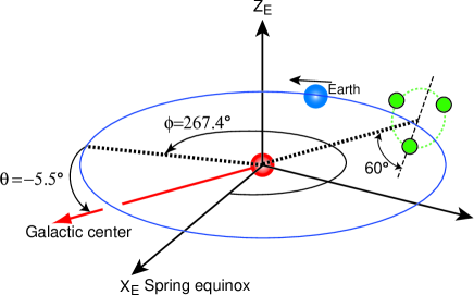
Figure 1: LISA configuration in the ecliptic coordinates. The Galactic center is at RA $267.4^{\circ}$ and dec. $-5.5^{\circ}$ in this coordinate system.

Let us now focus on the orbital motion of the LISA constellation (see Fig.1). The LISA orbital motion can be expressed by $\psi=-\omega t$, $\vartheta=-\pi/3$, $\varphi=\omega t$, where $\omega=2\pi/T_{0}$ is the orbital frequency of LISA ($T_{0}=1$ sidereal year) Since the antenna pattern function is periodic in time due to the orbital motion, the expected signals also vary in time with the same period $T_{0}$. It is therefore convenient to express the output signals by

$$\widetilde{C}_{IJ}(t,f)=\sum_{k=-\infty}^{+\infty}\,\,\widetilde{C}_{IJ,k}(f)\,\,e^{i\,k\,\omega\,t}.$$ (13)

Using the relation (11) with specific parameter set, the Fourier component $\widetilde{C}_{IJ,k}(f)$ is then given by

$$\tilde{C}_{k}(f) \equiv \frac{1}{T_{0}}\int^{T_{0}}_{0}dt~{}e^{-ik\omega t}\,\,\tilde{C}_{IJ}(t,f)$$ (14)

$$= \frac{1}{4\pi}\sum_{\ell=0}^{\infty}\sum_{m=-\ell}^{\ell-k}~{}[p_{\ell m}(f)]^{*}\,\,d^{\ell}_{(m+k),m}\left(-\frac{\pi}{3}\right)~{}a_{\ell,(m+k)}(f)$$

for $k\geq 0$. As for $k<0$, the lower and the upper limit of the sum over $m$ are changed to $m=-\ell-k$ and $m=\ell$, respectively.

Equation (14) as well as (5) is the theoretical basis to reconstruct the skymap of GWBs. Given the output data $\tilde{C}_{k}(f)$ (or $\tilde{C}_{IJ}(t,f)$) experimentally, the task is to solve the linear system (14) with respect to $p_{\ell m}(f)$ for given antenna pattern functions. One important remark deduced from equation (14) is that the accessible multipole coefficients $p_{\ell m}$ are severely restricted by the angular sensitivity of antenna pattern functions. The important properties of the antenna pattern functions are summarized in next subsection. Another important message is that the above linear systems are generally either over-constrained or under-determined. For the expression (14), if one truncates the multipole expansion with $\ell=\ell_{\mathrm{max}}$, the system consists of $\frac{1}{2}(\ell_{max}+1)(2\ell_{max}+1)$ unknowns and $N(2\ell_{max}+1)$ equations (for $k\geq 0$), where $N$ is the number of available modes of the antenna pattern functions. Thus this deconvolution problem is, in principle, over-determined for a relatively small truncation multipole $\ell_{\text{max}}$, while it becomes under-determined for a larger value of $\ell_{\text{max}}$. We will later discuss the over-determined case in Sec.IV.3.1, where $\ell_{\text{max}}=5$ and $N\simeq 5$.

II.2 Detector response and antenna pattern functions

Table 1: Important properties of antenna pattern function. Note that the cross-correlated data are blind to isotropic GWBs.

Combination of variables	Visible multipole moments in low-frequency regime $(\hat{f}\lesssim 1)$	General properties
(A,A), (E,E)	$\mathcal{O}(\hat{f}^{2}):$ $\ell=0,\,\,2,\,\,4$	visible only to $\ell=$even
(T,T)	$\mathcal{O}(\hat{f}^{4}):$ $\ell=0,\,\,4,\,\,6$	visible only to $\ell=$even
(A,E)	$\mathcal{O}(\hat{f}^{2}):$ $\ell=4$,  $\mathcal{O}(\hat{f}^{3}):$ $\ell=3,\,\,5$	blind to $\ell=0,\,\,1$
(A,T), (E,T)	$\mathcal{O}(\hat{f}^{3}):$ $\ell=1,\,\,3,\,\,5$	blind to $\ell=0$

The output signals of space interferometer sensitive to the gravitational waves are constructed by time-delayed combination of laser pulses. In the case of LISA, the technique to synthesize data streams canceling the laser frequency noise is known as time-delay interferometry (TDI), which is crucial for our subsequent analysis. In the present paper, we use the optimal set of TDI variables independently found by Prince et al. Prince et al. (2002) and Nayak et al.Nayak et al. (2003), which are free from the noise correlation . A simple realization of such data set is obtained from a combination of Sagnac signals, which are the six-link observables using all six LISA oriented arms. For example, the Sagnac signal S₁ measures the phase difference accumulated by two laser beams received at space craft $1$, each of which travels around the LISA array in clockwise or counter-clockwise direction. The explicit expression of detector tensor for such signal, which we denote by ${\bf D}_{\scriptscriptstyle\rm S_{1}}$, is given in equation (21) of Paper I (see also Cornish (2002b); Armstrong et al. (1999)). The analytic expression for other detector tensors ${\bf D}_{\rm S_{2}}$ and ${\bf D}_{\rm S_{3}}$ are also obtained by the cyclic permutation of the unit vectors $\mathbf{a},\,\mathbf{b}$ and $\mathbf{c}$.

Combining the three Sagnac signals, a set of optimal data combinations can be constructed Prince et al. (2002); Nayak et al. (2003) (see also Krolak et al. (2004)):

$${\bf D}_{\rm A}=\frac{1}{\sqrt{2}}({\bf D}_{\rm S_{3}}-{\bf D}_{\rm S_{1}}),$$

$${\bf D}_{\rm E}=\frac{1}{\sqrt{6}}({\bf D}_{\rm S_{1}}-2{\bf D}_{\rm S_{2}}+{\bf D}_{\rm S_{3}}),$$

$${\bf D}_{\rm T}=\frac{1}{\sqrt{3}}({\bf D}_{\rm S_{1}}+{\bf D}_{\rm S_{2}}+{\bf D}_{\rm S_{3}}).$$ (15)

These three detector tensors are referred to as $A,E,T$-variables, which generate six kinds of antenna pattern functions. Notice that in the equal arm-length limit, frequency dependence of these functions is simply expressed in terms of the normalized frequency:

$$\hat{f}\equiv\frac{f}{f_{*}},$$ (16)

where the characteristic frequency is given by $f_{*}=c/(2\pi L)$ with $L$ being the arm-length of detector. With the arm-length $L=5\times 10^{6}$ km, the characteristic frequency of LISA becomes $f_{*}\simeq 9.54$ mHz. In what follows, we use the analytic expressions for equal arm-length limit to demonstrate the reconstruction of GWB skymap. This is sufficient for the present purpose, because we are concerned with a fundamental theoretical basis to map-making capability of GWBs. The idea provided in the present paper would allow us to examine a more realistic situation and the same strategy can be applied to an extended analysis in the same manner.

Finally, we note that the antenna pattern functions for the optimal combinations of TDI have several distinctive features in angular sensitivity. In the low frequency limit ($\hat{f}\ll 1$), the antenna pattern functions for the self-correlations and the cross-correlations are expanded as

$${\mathcal{F}}_{AA}(f,\,\mathbf{\Omega})={} {\mathcal{F}}_{AA}^{(2)}(\mathbf{\Omega})\,\hat{f}^{2} +{} ~{}{\mathcal{F}}_{AA}^{(4)}(\mathbf{\Omega})\,\hat{f}^{4} +~{}O(\hat{f}^{6})$$ (17)

$${\mathcal{F}}_{TT}(f,\,\mathbf{\Omega})={} ~{}{\mathcal{F}}_{TT}^{(4)}(\mathbf{\Omega})\,\hat{f}^{4} +~{}O(\hat{f}^{6})$$

$${\mathcal{F}}_{AE}(f,\,\mathbf{\Omega})={} {\mathcal{F}}_{AE}^{(2)}(\mathbf{\Omega})\,\hat{f}^{2} +{} ~{}{\mathcal{F}}_{AE}^{(3)}(\mathbf{\Omega})\,\hat{f}^{3} +{} ~{}{\mathcal{F}}_{AE}^{(4)}(\mathbf{\Omega})\,\hat{f}^{4} +~{}O(f^{5})$$

$${\mathcal{F}}_{AT}(f,\,\mathbf{\Omega})={} ~{}{\mathcal{F}}_{AT}^{(3)}(\mathbf{\Omega})\,\hat{f}^{3} +{} ~{}{\mathcal{F}}_{AT}^{(4)}(\mathbf{\Omega})\,\hat{f}^{4} +~{}O(\hat{f}^{5})$$

The frequency dependence of ${\mathcal{F}}_{EE}$ and ${\mathcal{F}}_{ET}$ are the same as for ${\mathcal{F}}_{AA}$ and ${\mathcal{F}}_{AT}$, respectively. Since the leading term of the TT-correlation is $O(\hat{f}^{4})$, the $TT$-correlation becomes insensitive to the gravitational waves in the low-frequency regime. We will use all correlated data set except for the $TT$-correlation. In Table 1, we summarize the important properties for the multipole moments of antenna pattern functions. Also, in Appendix A, employing the perturbative approach based on the low-frequency approximation $\hat{f}\ll 1$, the spherical harmonic expansion for antenna pattern functions are analytically computed, which will be useful in subsequent analysis.

III Perturbative reconstruction method for GWB skymap

We are in position to discuss the methodology to reconstruct a skymap of GWB based on the expression (14) (or (5)). Since we are specifically concerned with low-frequency sources observed via LISA, it would be helpful to employ a perturbative approach using the low-frequency expansion of antenna pattern function. In Sec.III.1, owing to the expression (14), a perturbative reconstruction method is presented. Sec.III.2 discusses alternative reconstruction method based on the time-series representation (5).

III.1 General scheme

Hereafter, we focus on the GWBs in the low-frequency band of the detector, the wavelength of which is typically longer than the arm-length of the gravitational detector, i.e., $\hat{f}\lesssim 1$. Without loss of generality, we restrict our attention to the reconstruction of a GWB skymap in a certain narrow frequency range, $f\sim f+\Delta f$, within which a separable form of the GWB spectrum is a good assumption:

$$S_{h}(f,\mathbf{\Omega})=H(f)\,\,P(\mathbf{\Omega}).$$ (18)

Further, for our interest of the narrow bandwidth, it is reasonable to assume that the spectral density $H(f)$ is described by a power-law form as $H(f)={\mathcal{N}}\,f^{\alpha}$. In the reconstruction analysis discussed below, the spectral index $\alpha$ is assumed to be determined beforehand from theoretical prediction and/or experimental constraint .

In the low frequency approximation up to the order $\mathcal{O}(\hat{f}^{3})$, we have five output signals which respond to the GWBs, i.e., $AA$-, $EE$-, $AE$-, $AT$- and $ET$-correlations, each output of which is represented by equation (14). Collecting these linear equations and arraying them appropriately, the linear algebraic equations can be symbolically written in a matrix form as

$${\mathbf{c}}(f)={\mathbf{A}}(f)\cdot{\mathbf{p}}.$$ (19)

In the above expression, while the vector ${\mathbf{p}}$ represents the unknowns consisting of the multipole coefficients of GWBs $p_{\ell m}$, the vector ${\mathbf{c}}(f)$ contains the correlation signals $\tilde{C}_{k}(f)$. Here, the frequency dependence of the function $H(f)$ has been already factorized and thereby the vector ${\mathbf{p}}$ only contains the information about the angular distribution. The matrix ${\mathbf{A}}(f)$ is the known quantity consisting of the multipole coefficients of each antenna pattern and the Wigner $D$ matrices (see Appendix C for an explicit example).

As we have already mentioned, the linear systems (19) become either over-determined or under-determined system. In most of our treatment in the low-frequency regime, the linear systems (19) tend to become over-determined, but this is not always correct depending on the amplitude of GWB spectrum $H(f)$ (see Sec.IV.2). In any case, the matrix $\mathbf{A}$ would not be a square matrix and the number of components of the vector $\mathbf{c}$ does not coincide with the one in the vector $\mathbf{p}$. In the over-determined case, while there is a hope to get a unique solution $\mathbf{p}$ to produce the gravitational-wave signal $\mathbf{c}$, it seems practically difficult due to the errors associated with the instrumental noise and/or numerical analysis. Hence, instead of pursuit of a rigorous solution, it would be better to focus on the issue how to get an approximate solution by a simple and systematic method.

In the case of our linear system, the approximate solution for the multipole coefficient $\mathbf{p}_{\rm approx}$ can be obtained from the least-squares method in the following form:

$$\mathbf{p}_{\rm\scriptscriptstyle approx}=\mathbf{A}^{+}\cdot\mathbf{c}.$$ (20)

The matrix $\mathbf{A}^{+}$ is called the pseudo-inverse matrix of Moore-Penrose type, whose explicit expression can be uniquely determined from the singular value decomposition (SVD) Press et al. (2002). According to the theorem of linear algebra, the matrix $\mathbf{A}$, whose number of rows is greater than or equal to its number of columns, can be generally written as $\mathbf{A}=U^{T}\cdot\mbox{diag}[w_{i}]\cdot V$. Here, the matrices $U$ and $V$ are orthonormal matrices which satisfy $U^{\dagger}\,U=V^{\dagger}\,V=\mathbf{1}$, where the quantity with subscript ^† represents the Hermite conjugate variable. The quantity $\mbox{diag}[w_{i}]$ represents an diagonal matrix with singular values $w_{i}$ with respect to the matrix $\mathbf{A}$. Then the pseudo-inverse matrix becomes

$$\mathbf{A}^{+}=V^{T}\cdot\mbox{diag}[w_{i}^{-1}]\cdot U.$$ (21)

It should be stressed that the explicit form of the pseudo-inverse matrix $\mathbf{A}^{+}$ is characterized only by the angular dependence of antenna pattern functions.

In principle, the least-squares method by SVD can work well and all the accessible multipole moments of GWB would be obtained as long as the antenna pattern functions have the corresponding sensitivity to each detectable multipole moment. As we mentioned in Sec.II.2, however, the angular power of antenna pattern function depends sensitively on the frequency. In the low-frequency regime, the frequency dependence of the non-vanishing multipole moments appears at $\mathcal{O}(\hat{f}^{2})$ for $\ell=0,\,\,2$ and $4$, and $\mathcal{O}(\hat{f}^{3})$ for $\ell=1,\,\,3$ and $5$ (see Table 1). In this respect, by a naive application of the least-squares method, it is difficult to extract the information about $\ell=$odd modes of GWBs because the singular values of the matrix $\mathbf{A}$ are dominated by the lowest-order contribution of the antenna pattern functions.

For a practical and a reliable estimate of the odd multipoles in low-frequency regime, the least-squares method should be applied combining with the perturbative scheme described below. Let us recall from the expression (17) that the matrix $\mathbf{A}$ can be expanded as

$$\mathbf{A}=\hat{f}^{2}\,\,\mathbf{A}^{(2)}+\hat{f}^{4}\,\,\mathbf{A}^{(4)}+\cdots$$ (22)

for a matrix consisting of the self-correlation signals $\mathcal{F}_{AA}$ and $\mathcal{F}_{EE}$,

$$\mathbf{A}=\hat{f}^{2}\,\,\mathbf{A}^{(2)}+\hat{f}^{3}\,\,\mathbf{A}^{(3)}+\hat{f}^{4}\,\,\mathbf{A}^{(4)}+\cdots$$ (23)

for a matrix consisting of the cross-correlation signal $\mathcal{F}_{AE}$, and

$$\mathbf{A}=\hat{f}^{3}\,\,\mathbf{A}^{(3)}+\hat{f}^{4}\,\,\mathbf{A}^{(4)}+\cdots$$ (24)

for a matrix consisting of the cross-correlation signals $\mathcal{F}_{AT}$ and $\mathcal{F}_{ET}$. Then the resultant matrices $\mathbf{A}^{(i)}$ become independent of the frequency. The above perturbative expansion implies that the output signal $\mathbf{c}$ is also expanded in powers of $\hat{f}$. Since the frequency dependence of the function $H(f)$ has been already factorized in equation (19), we have

$$\mathbf{c}(f)=\left\{\begin{array}[]{lll}&\hat{f}^{2}~{}\mathbf{c}^{(2)}+\hat{f}^{4}\mathbf{c}^{(4)}+\cdots,&\text{for AA-, EE-correlations}\\ \\ &\hat{f}^{2}~{}\mathbf{c}^{(2)}+\hat{f}^{3}~{}\mathbf{c}^{(3)}+\hat{f}^{4}\mathbf{c}^{(4)}+\cdots,&\text{for AE-correlation}\\ \\ &\hat{f}^{3}~{}\mathbf{c}^{(3)}+\hat{f}^{4}\mathbf{c}^{(4)}+\cdots,&\text{for AT-,ET-correlations}\end{array}\right.$$ (30)

Substituting the terms (22)-(24) and (30) into the expression (19) and collecting the terms of each order of $\hat{f}$, we have

$$\mathbf{c}^{(i)}=\mathbf{A}^{(i)}\,\cdot\,\mathbf{p}^{(i)},\quad\quad(i=2,\,\,3,\,\,4,\,\,\cdots)$$ (31)

where the subscript ⁽ⁱ⁾ means the quantity consisting of the order $\mathcal{O}(\hat{f}^{i})$ terms. The vector $\mathbf{p}^{(i)}$ represents the accessible multipole moments $p_{\ell m}$ to which the antenna pattern functions become sensitive in this order. For example, the vector $\mathbf{p}^{(2)}$ contains the $\ell=0,\,2$ and $4$ modes, while the vector $\mathbf{p}^{(3)}$ have the multipole moments with $\ell=1,\,3$ and $5$. Since the expression (31) has no explicit frequency dependence, we can reliably apply the least-squares solution by the SVD to reconstruct the odd modes of GWBs, as well as the even modes:

$$\mathbf{p}^{(i)}_{\rm\scriptscriptstyle approx}=[\mathbf{A}^{(i)}]^{+}\,\cdot\,\mathbf{c}^{(i)}.$$ (32)

Each step of the perturbative reconstruction scheme is summarized in Fig. 2 (see Appendix C in more details).

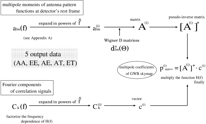
Figure 2: Flowchart of perturbative reconstruction scheme based on the harmonic-Fourier representation.

Finally, we note that the low-frequency reconstruction method presented here assumes the perturbative expansion form of the output signal $\mathbf{c}$. To determine the coefficients $\mathbf{c}^{(i)}$ in equation (30), one must know the frequency dependence of the vector $\mathbf{c}$ in the narrow bandwidth $f\sim f+\Delta f$, which can be achieved by analyzing the multi-frequency data. One important remark is that the signal-to-noise ratio in each reconstructed multipoles might be influenced by the sampling frequencies and/or the data analysis strategy. This point will be discussed later in Sec. IV.3.

III.2 Reconstruction based on the time-series representation

So far, we have discussed the reconstruction method based on the harmonic-Fourier representation (14). The main advantage of the harmonic-Fourier representation is that it gives a simple algebraic equation suitable for applying the least-squares solution by SVD. However, the harmonic-Fourier representation implicitly assumes that the space interferometer orbits around the sun under keeping their configuration rigidly. In reality, rigid adiabatic treatment of the spacecraft motion is no longer valid due to the intrinsic variation of arm-length caused by the Keplerian motion of three space crafts, as well as the tidal perturbation by the gravitational force of solar system planets Cornish and Hellings (2003); Tinto et al. (2004); Shaddock (2004). In a rigorous sense, the time dependence of antenna pattern function cannot be described by the Euler rotation of antenna pattern function at rest frame (see footnote 2). Although the influence of arm-length variation is expected to be small in the low-frequency regime, alternative approach based on the other representation would be helpful to consider the GWB skymap beyond the low-frequency regime.

Here, we briefly discuss the reconstruction method based on the time-series representation (5). The time-series representation is mathematically equivalent to the harmonic-Fourier representation under the rigid adiabatic treatment, but in general, no additional assumption for space craft configuration is invoked to derive the expression (5), except for the premise that the time-dependence of the antenna pattern functions, i.e., the motion of each spacecraft, is well-known theoretically and/or observationally. Moreover, as we see below, the method based on the time-series representation allows us to reconstruct directly the skymap $S_{h}$, without going through intermediate variables, e.g. $p_{\ell m}$. In this sense, the time-series representation would be superior to the harmonic-Fourier representation for practical purpose, although there still remains the same problem as discussed in Appendix B concerning the degeneracy of the multipole coefficients.

In principle, the perturbative reconstruction scheme given in Sec.III.1 can be applicable to the map-making problem based on the time-series representation. To apply this, we discretize the integral expression (5) so as to reduce it to a matrix form like equation (19). For example, we discretize the celestial sphere $(\theta,\,\phi)$ into a regular $N$ meshes and also the continuous time-series into the regular $M$ grids. Then we have

$$\widetilde{C}(t_{i},\,f)=\sum_{j=1}^{N}\,\,S_{h}(|f|,\,\,\mathbf{\Omega}_{j})\,\,\mathcal{F}^{E}(f,\,\mathbf{\Omega}_{j};\,t_{i})\,\frac{\Delta\mathbf{\Omega}_{j}}{4\pi},\quad(i=1,2,\cdots,\,M),$$ (33)

where $\Delta\mathbf{\Omega}_{i}=\sin\theta_{i}\,\Delta\theta_{i}\,\Delta\phi_{i}$. Here, we have ignored the noise contribution and dropped the subscript _IJ. For a reconstruction of low-frequency skymap, a large number of mesh and/or grid are not necessary. Typically, for the angular resolution up to $\ell=5$, it is sufficient to set $M=16$ and $N=16$ (see Sec.IV.3). The above discretization procedure is repeated for the five output data of the correlation signals. Then, simply following the same procedure as in the case of the harmonic-Fourier representation, the least-squares method by SVD is applied to get the luminosity distribution of GWBs. Note that the meanings of the matrix $\mathbf{A}^{(i)}$, the vectors $\mathbf{c}^{(i)}$ and $\mathbf{p}^{(i)}$ in the perturbative expansion are appropriately changed as follows. For the matrix $\mathbf{A}^{(i)}$, we have

$$\mathbf{A}^{(i)}=\frac{1}{4\pi}\left(\begin{array}[]{cccc}\mathcal{F}^{(i)}(\mathbf{\Omega}_{1},t_{1})\,\Delta\mathbf{\Omega}_{1}&\mathcal{F}^{(i)}(\mathbf{\Omega}_{2},t_{1})\,\Delta\mathbf{\Omega}_{2}&\cdots&\mathcal{F}^{(i)}(\mathbf{\Omega}_{N},t_{1})\,\Delta\mathbf{\Omega}_{N}\\ \mathcal{F}^{(i)}(\mathbf{\Omega}_{1},t_{2})\,\Delta\mathbf{\Omega}_{1}&\mathcal{F}^{(i)}(\mathbf{\Omega}_{2},t_{2})\,\Delta\mathbf{\Omega}_{2}&\cdots&\mathcal{F}^{(i)}(\mathbf{\Omega}_{N},t_{2})\,\Delta\mathbf{\Omega}_{N}\\ \vdots&\vdots&\ddots&\vdots\\ \mathcal{F}^{(i)}(\mathbf{\Omega}_{1},t_{M})\,\Delta\mathbf{\Omega}_{1}&\mathcal{F}^{(i)}(\mathbf{\Omega}_{2},t_{M})\,\Delta\mathbf{\Omega}_{2}&\cdots&\mathcal{F}^{(i)}(\mathbf{\Omega}_{N},t_{M})\,\Delta\mathbf{\Omega}_{N}\\ \end{array}\right),\quad\quad(i=2,\,3,\,\cdots)$$ (34)

The corresponding vectors $\mathbf{c}_{(i)}$ and $\mathbf{p}_{(i)}$ becomes

$$\mathbf{c}^{(i)}=\left(\begin{array}[]{c}\widetilde{C}^{(i)}(t_{1})\\ \widetilde{C}^{(i)}(t_{2})\\ \vdots\\ \widetilde{C}^{(i)}(t_{M})\end{array}\right),\qquad\mathbf{p}^{(i)}=\left(\begin{array}[]{c}S_{h}^{(i)}(\Omega_{1})\\ S_{h}^{(i)}(\Omega_{2})\\ \vdots\\ S_{h}^{(i)}(\Omega_{N})\\ \end{array}\right),$$ (35)

where $\widetilde{C}^{(i)}(t)$ and $S_{h}^{(i)}(\Omega)$ the perturbative coefficients of $\widetilde{C}(t,f)$ and $S_{h}(|f|,\Omega)$ in power of $\hat{f}^{i}$, respectively. Using these expressions, the least-squares solution is constructed as $\mathbf{p}_{\rm approx}=\mathbf{p}_{\rm approx}^{(2)}+\mathbf{p}_{\rm approx}^{(3)}+\cdots$, with a help of equation (32). Then, the resultant expression $\mathbf{p}_{\rm approx}$ directly gives a GWB skymap in the ecliptic coordinate, i.e., $S_{h}(|f|,\,\mathbf{\Omega})$, not the multipole coefficients.

IV Demonstration: skymap of Galactic background

Perturbative reconstruction scheme presented in the previous section is applicable to a general map-making problem for any kind of GWB sources. In this section, to see how our general scheme works in practice, we demonstrate the reconstruction of a GWB skymap focusing on a specific source of anisotropic GWB. An interesting example for LISA detector is a confusion-noise background produced by the Galactic population of unresolved binaries. After describing a model of Galactic GWB in Sec.IV.1, the expected signals for time-modulation data of self- and cross-correlated TDIs are calculated in Sec.IV.2. Based on these, the detectable Fourier components for time-modulation signals are discussed evaluating the signal-to-noise ratios. In Sec.IV.3, a reconstruction of the GWB skymap is performed based on the harmonic-Fourier representation and the time-series representation. The resultant values of the multipole coefficients for Galactic GWBs are compared with those from the full-resolution skymap, taking account of the influence of the noises.

IV.1 A model of Galactic GWB

For our interest of GWBs in the low-frequency regime with $f\lesssim f_{*}\simeq 9.54$ mHz, it is reasonable to assume that the anisotropic GWB spectrum $S_{h}(f,\mathbf{\Omega})$ is separately treated as $S_{h}(f,\mathbf{\Omega})=H(f)\,P(\mathbf{\Omega})$, as we mentioned. The power spectral density $H(f)$ is approximated by a power-law function like $H(f)={\mathrm{N}}\,f^{\alpha}$, whose amplitude will be explicitly given later. For illustrative purpose, we consider the simplest model of luminosity distribution $P(\mathbf{\Omega})$, in which the Galactic GWB is described by an incoherent superposition of gravitational waves produced by compact binaries whose spatial structure just traces the Galactic stellar distribution observed via infrared photometry. We use the fitting model of Galactic stellar distribution given in Binney et al. (1997), which consists of triaxial bulge and disk components (see also Seto (2004)). The explicit functional form of the density distribution $\rho(\mathbf{x})$ written in the Galactic coordinate system becomes

$$\rho(\mathbf{x})=\rho_{\rm disk}(\mathbf{x})+\rho_{\rm bulge}(\mathbf{x})\,\,;$$ (36)

$$\quad\rho_{\rm bulge}=\frac{\rho_{0}}{(1+a/a_{0})^{1.8}}\,\,e^{-(a/a_{\rm m})^{2}},$$

$$\quad\rho_{\rm disk}=\left(\frac{e^{-|z|/z_{0}}}{z_{0}}+\alpha\,\frac{e^{-|z|/z_{1}}}{z_{1}}\right)\,R_{s}\,e^{-R/R_{\rm s}}$$

with the quantities $a$ and $R$ defined by $a\equiv[x^{2}+(y/\eta)^{2}+(z/\zeta)^{2}]^{1/2}$ and $R\equiv(x^{2}+y^{2})^{1/2}$. Note that the $z$-axis is oriented to the north Galactic pole and the direction of the $x$-axis is $20^{\circ}$ different from the Sun-center line. Here the parameters are given as follows: $\rho_{0}=624$, $a_{\rm m}=1.9$ kpc, $a_{0}=100$ pc, $R_{\rm s}=2.5$ kpc, $z_{0}=210$ pc, $z_{1}=42$ pc, $\alpha=0.27$, $\eta=0.5$ and $\zeta=0.6$. Provided the three-dimensional structure of stellar distribution $\rho(\mathbf{x})$, the angular distribution $P(\mathbf{\Omega})$ is obtained by projecting it onto the sphere in observed frame, i.e., ecliptic coordinate:

$$P(\mathbf{\Omega})=C\,\int dr\,\,4\pi\,r^{2}\,\,\frac{\rho(r,\mathbf{\Omega})}{r^{2}},$$ (37)

where $C$ is a numerical constant normalized by $\int d\mathbf{\Omega}\,P(\mathbf{\Omega})=1$. The integration over $r$ is performed along a line-of-sight direction from a location of space interferometer to infinity.

In Fig.3, the projected intensity distribution of GWB is numerically obtained specifically in ecliptic coordinate and it is then transformed into Galactic coordinate, shown as the Hammer-Aitoff map. A strong intensity peak is found around the Galactic center and the disk-like structure can be clearly seen. Notice that while the result depicted in Fig.3 represents a full-resolution skymap, it cannot be attained from the perturbative reconstruction scheme in low-frequency regime. For the antenna pattern functions of cross-correlated TDI signals up to the order $\mathcal{O}(\hat{f}^{3})$, the detectable multipole moments of GWB are limited to $\ell\leq 5$. Moreover, in the low-frequency limit $\mathcal{O}(\hat{f}^{2})$, only the even modes $\ell=0$, $2$ and $4$ are measurable. Thus, the reconstructed skymap would be rather miserable compared to the full skymap which contains the higher multipoles $\ell\gtrsim 30$ (see Fig.12 in Appendix). Taking account of these facts, in right panel of Fig.4, we plot the low-resolution skymap, which was obtained from the full-resolution skymap just dropping the higher multipole moments with $\ell>5$. In Appendix D, with a help of the Fortran package of spherical harmonic analysis (Adams and Swarztrauber (2003), see Appendix D), the numerical values of the multipole coefficients $p_{\ell m}$ up to $\ell=5$ are computed and are summarized in Table 3. Also in the left panel, the odd modes are further subtracted and the remaining multipole moments are only $\ell=0$, $2$ and $4$. As a result, the fine structure around the bulge and the disk components is coarse-grained and the intensity of the GWB diminishes. It also shows some fake patterns with negative intensity. Nevertheless, one can clearly see the anisotropic structure of GWB , which is mainly contributed from the gravitational-wave sources around the Galactic disk. With a perturbative reconstruction of low-frequency up to $\mathcal{O}(\hat{f}^{3})$, one can roughly infer that the main sources of Galactic GWB comes from the Galactic center.

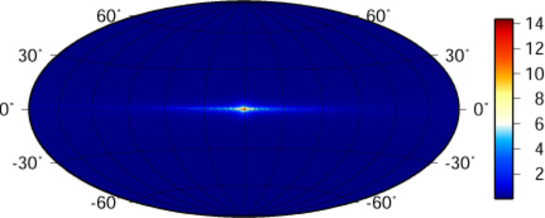
Figure 3: Full-resolution skymap of the Galactic gravitational-wave background shown as Hammer-Aitoff map in Galactic coordinate.

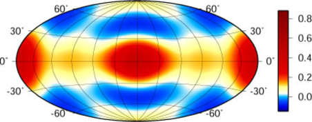
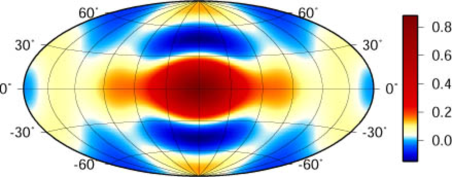
Figure 4: Expected images of GWB skymap by LISA based on the low-frequency reconstruction scheme, which are both depicted in the Galactic coordinate. Left: low-resolution skymap created by truncating all the multipoles except for $\ell=0$, $2$ and $4$ from the original full-resolution skymap. Right: skymap created by truncating the higher multipoles $\ell>6$.

IV.2 Time-modulation signals and signal-to-noise ratio

Given the intensity distribution of GWB, one can calculate the cross-correlation signals observed via LISA, which are inherently time-dependent due to the orbital motion of the LISA detector. The effect of the annual modulation of the Galactic binary confusion noise on the LISA data analysis had been previously studied in Seto (2004) in the low-frequency limit $\hat{f}\ll 1$. Recently, Monte Carlo simulations of Galactic GWB were carried out by several groups and the annual modulation of GWB intensity has been confirmed in a realistic setup with specific detector output Benacquista et al. (2004); Edlund et al. (2005); Timpano et al. (2005).

Owing to the expression (5), the time-modulation signals $\widetilde{C}(t,f)$ neglecting the instrumental noises are computed for optimal TDIs at the frequency $\hat{f}=0.1$, i.e., $f\simeq 1\mathrm{mHz}$ using the full expression of antenna pattern function (7). The results are then plotted as function of orbital phase. In Fig. 5, six outputs of the self- and cross-correlation signals normalized to its time-averaged value, $\widetilde{C}(t,f)/|\widetilde{C}_{0}(f)|$ are shown. The solid and dashed lines denote the real and imaginary parts of the correlation signals, respectively.

The time modulation of these outputs basically reflects the spatial structure of GWB. As LISA orbits around the Sun, the direction normal to LISA’s detector plane, which is the direction sensitive to the gravitational waves, sweeps across the Galactic plane. Since the response of the LISA detector to the gravitational waves along the $\mathbf{\hat{\Omega}}$ direction give the same response to the waves along the $-\mathbf{\hat{\Omega}}$ direction (see Eq.(9) and the brief comment there), the time-modulation signal is expected to have a bimodal structure, like $AA$- and $EE$-correlations. However, the actual modulation signals are more complicated, depending on the angular sensitivity of their antenna pattern functions, as well as the observed frequency. Further, the cross-correlation data can be generally complex variables, whose behaviors are different between real- and imaginary-parts.

Figure 5: Annual time-modulation signals of self- and cross-correlation data as function of orbital phase assuming the observed frequency $\hat{f}=0.1$, i.e., $f\simeq 1\mathrm{mHz}$. Here, the correlation signals $\widetilde{C}_{IJ}(t,f)$ are plotted normalizing with $k=0$ component of correlation signal $\widetilde{C}_{IJ,0}(f)$. Solid and dashed lines represent the real and the imaginary part of correlation signal, respectively.

Notice that the time-modulation signals presented in Fig. 5 are the results in an idealistic situation free from the noise contribution. In presence of the random noise, some of the correlation data which contain gravitational wave signals are overwhelmed by noise, which cannot be used for the reconstruction of GWB skymap. Hence, one must consider the signal-to-noise ratio (SNR) to discriminate available correlation data. To evaluate this, the output signals depicted in Fig.5 are first transformed to its Fourier counterpart, $\widetilde{C}_{k}(f)$. The resultant Fourier components for each signal are then compared to the noise contributions. The SNR for each component is expressed in the following form (Seto and Cooray (2004), see also Giampieri and Polnarev (1997a); Ungarelli and Vecchio (2001b)):

$$\left(\frac{S}{N}\right)_{k}=\sqrt{2\,\,\Delta f\,\,T}\,\,\frac{|\widetilde{C}_{k}|}{N_{k}}.$$ (38)

Here we set the observational time to $T=10^{8}$sec and the bandwidth to $\Delta f=10^{-3}$Hz. The quantity $N_{k}$ represents the noise contribution. The important remark is that the noise contribution comes from not only the detector noise but also the randomness of the signal itself. The details of the analytic expression for $N_{k}$ will be given elsewhere Kudoh and Taruya (2005b). Here, as a crude estimate, we evaluate the noise contribution $N_{k}$ as

$$N_{k}=\sqrt{2\,\,\Delta f\,\,T}\,\,S_{n}^{II},\quad(I=A,~{}E,~{}T)$$ (39)

for $k=0$ component of self-correlation signals and

$$N_{k}=\sqrt{\mbox{max}\left(\widetilde{C}_{II,0}\widetilde{C}_{JJ,0},~{}\widetilde{C}_{II,0}S_{n}^{JJ},~{}\widetilde{C}_{JJ,0}S_{n}^{II},~{}S_{n}^{II}S_{n}^{JJ}\right)},\quad(I,J=A,~{}E,~{}T)$$ (40)

for cross-correlation signals and $k\neq 0$ component of self-correlation signals. To estimate SNR, one further needs the spectral density for instrumental noise, i.e., $S_{n}^{\scriptscriptstyle\rm AA}(f)$, $S_{n}^{\scriptscriptstyle\rm EE}(f)$ and $S_{n}^{\scriptscriptstyle\rm TT}(f)$. We use the expressions given in equation (58) of Paper I (see also Cornish (2002b); Prince et al. (2002)) . Note that all the cross-correlated noise spectra such as $S_{n}^{\scriptscriptstyle\rm AE}(f)$ and $S_{n}^{\scriptscriptstyle\rm AT}(f)$ are exactly canceled.

In Fig.6, the SNRs for six output data are evaluated and are shown in the histogram as function of Fourier component, $k$. In these panels, thick-dotted lines show the detection limit of $(S/N)_{k}=5$, while the thin-dotted lines mean $(S/N)_{k}=1$. When evaluating the SNR, we specifically consider the two cases:

Case A:

realistic case in which the rms amplitude of GWB spectrum is given by $S_{h}^{1/2}=5\times 10^{-19}$Hz^-1/2 at the frequency $f=1$mHz .

Case B:

optimistic case in which the rms amplitude of GWB spectrum is ten times larger than that in the realistic case, i.e., $S_{h}^{1/2}=5\times 10^{-18}$Hz^-1/2 at $f=1$mHz.

The results of SNR are then shown in solid (case A) and dashed lines (case B), respectively.

As anticipated from the sensitivity of antenna pattern function in Table 1, the SNR for $TT$-correlation is much less than unity. Even in the optimistic case, the SNR is about ten times smaller than unity and thus the $TT$-correlation data cannot be used for reconstruction of the GWB skymap. Apart from this, the SNRs for the self-correlation signals $AA$ and $EE$ as well as for the cross-correlation signal $AE$ are generally good compared to the cross-correlation data $AT$ and $ET$. With sufficient higher SNR of $(S/N)_{k}\geq 5$, the available Fourier components of $AA$-, $EE$- and $AE$-correlations become $k=-2,\,-1,\,0,\,+1,\,+2$ in both realistic and optimistic cases. This is consistent with the previous estimates Seto and Cooray (2004). On the other hand, with a large amplitude of GWB spectrum (case B), only the $k=0$ component is accessible in the signal combinations of $AT$ and $ET$. This is mainly due to the fact that the sensitivity of the $T$-variable is poor at low-frequency and thereby the noise contribution $N_{k}$ becomes $\{\widetilde{C}_{AA,0}S_{n}^{\rm\scriptscriptstyle TT}\}^{1/2}$ or $\{\widetilde{C}_{EE,0}S_{n}^{\rm\scriptscriptstyle TT}\}^{1/2}$, which is much larger than $\{\widetilde{C}_{AA,0}\widetilde{C}_{TT,0}\}^{1/2}$ or $\{\widetilde{C}_{EE,0}\widetilde{C}_{TT,0}\}^{1/2}$.

Thus, the available Fourier components of correlation data used for the reconstruction of the skymap would be severely restricted in practice. Under such restricted situation, the deconvolution problem of the linear system (14) tends to be under-determined. Nevertheless, as it will be shown below, one can determine the $\ell=0$, $2$ and $4$ modes of multipole coefficients of the Galactic GWB with sufficiently small errors. In addition, with the $k=0$ components of $AT$- and $ET$-correlations, the odd moments $\ell=1$ and $3$ can be recovered.

Figure 6: Signal-to-noise ratio for each Fourier component of correlation signals, $(S/N)_{k}$ estimated at $\hat{f}=0.1$ ($f\simeq 1$mHz). The histogram depicted in solid line indicates the case with the amplitude of Galactic GWB given by $S_{h}^{1/2}=5\times 10^{-19}$Hz^-1/2 at $f=1$mHz (case A), while the histogram in dashed line represents the signal-to-noise ratio for the case with $S_{h}^{1/2}=5\times 10^{-18}$Hz^-1/2 (case B). The thin-dashed, and thick-dashed lines respectively denote the lines of $(S/N)_{k}=1$ and $5$.

IV.3 Reconstruction of a skymap

Keeping the remarks on the SNR estimation in previous subsection in mind, we now proceed to a reconstruction analysis and test the validity of perturbative reconstruction method presented in Sec. III. For this purpose, in addition to the analysis in the under-constrained cases (case A and B) mentioned above, we also consider the over-constrained case as an illustrative example.

Table 2: Components of $\widetilde{C}_{k}$ used for reconstruction analysis based on the harmonic-Fourier representation

	AA	EE	TT	AE	AT	ET
Over-determined case	$-2\leq k\leq+2$	$-2\leq k\leq+2$	none	$-8\leq k\leq+8$	$-4\leq k\leq+4$	$-4\leq k\leq+4$
Under-determined case
case A	$-2\leq k\leq+2$	$-2\leq k\leq+2$	none	$-2\leq k\leq+2$	none	none
case B	$-2\leq k\leq+2$	$-2\leq k\leq+2$	none	$-2\leq k\leq+2$	$k=0$	$k=0$

IV.3.1 Over-determined case

(I) Harmonic-Fourier representation  Let us first focus on a very idealistic situation that the noise contributions are entirely neglected. In such a case, all the components of self- and cross-correlation data $\widetilde{C}_{k}$ are available to the reconstruction analysis. In practice, however, it is sufficient to consider some restricted components among all available data. Here, to make a skymap with multipoles of $\ell\leq 5$, we use the $k=-2\sim+2$ components of self-correlation signals $AA$ and $EE$, the $k=-4\sim+4$ components of cross-correlation signals $AT$ and $ET$, and $k=-8\sim+8$ components of $AE$-signal (see Table 2). Even in this case, the linear system (14) is still over-determined and the least-squares approximation by SVD is potentially powerful to obtain the multipole coefficients of anisotropic GWB. The procedure of reconstruction analysis is the same one as presented in Fig.2. For the output signals of harmonic-Fourier representation, we use the data $\widetilde{C}_{k}$ observed at the frequencies $\hat{f}=0.05$ and $0.15$, in addition to the data for our interest at $\hat{f}=0.1$. Collecting these multi-frequency data, the perturbative expansion form of the vector $\mathbf{c}(f)$ is specified up to the third order in $\hat{f}$ and the coefficients $\mathbf{c}^{(i)}$ are determined (Appendix C).

In Fig.7, the reconstructed results of multipole coefficients $p_{\ell m}$ are converted to the projected intensity distribution (9) and are shown as Hammer-Aitoff map in Galactic coordinate. Left panel shows the skymap reconstructed from the lowest-order signals of self- and cross-correlation data $\mathbf{c}^{(2)}$, which only includes the $\ell=0$, $2$ and $4$ modes, while right panel is the result taking account of the leading-order correction $\mathbf{c}^{(3)}$. Comparing those with the expected skymap shown in Fig.4, the reconstruction seems almost perfect. In Fig. 8, numerical values of the reconstructed multipole coefficients are compared with the true values listed in Table 3. The agreement between the reconstruction results (open circles) and the true values (crosses) is quite good and the fractional errors are well within a few percent except for $p_{20}$ and $p_{50}$. A remarkable fact is that the monopole and the quadrupole values can be reproduced reasonably well despite the presence of the degeneracy mentioned in Appendix.B. This is just an accidental result. The (small) discrepancy in the “recovered” $p_{20}$ can be ascribed to the expression (56). After all, the least-squares method by SVD provides a robust reconstruction method when the linear system (14) becomes over-determined.

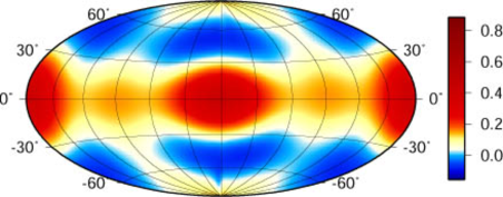
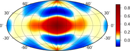
Figure 7: Reconstructed skymap from the time-modulation signals in the over-determined case. The results were obtained by the method based on harmonic-Fourier representation and are plotted in the Galactic coordinate. The left panel shows the leading-order result, where $\ell=0$, $2$ and $4$ modes are only reconstructed, while the right panel represents the result including all reconstructed multipoles ($\ell\leq 5$).

Figure 8: Reconstructed values of multipole coefficients $|p_{\ell m}|$ in over-determined case. These numerical values are evaluated in the ecliptic frame. The open circles represent the reconstruction results, while the crosses mean the true values, which are obtained from the spherical harmonic expansion of full-resolution skymap (see Table 3).

(II) Time-series representation  The successful reconstruction of the GWB skymap can also be achieved by the alternative approach based on the time-series representation (5). Following the procedure presented in Sec.III.2, the intensity skymap of the GWB is directly obtained and the results taking account of the lowest-order and the leading-order contributions to the antenna pattern functions are shown in left and right panels in Fig.9, respectively. Here, to create the discretized data set (33), the number of grid and/or mesh was specified as $M=16$ in time and $N=17\times 32$ in spherical coordinate. The time-series data of antenna pattern functions were numerically generated based on the full analytic expressions given in Sec.II.2 under assuming that the arm-length of the three space crafts are rigidly kept fixed. The reconstructed skymap reasonably agrees with Fig.7 as well as Fig.4. Although the situation considered here is very idealistic and thus the results in Fig.9 should be regarded as just a preliminary one, one expects that the methodology based on the time-series representation is potentially powerful even when the rigid adiabatic treatment of space craft motion becomes inadequate. To discuss its effectiveness, a further investigation is needed. The details of the analysis including the effects of arm-length variation will be presented elsewhere.

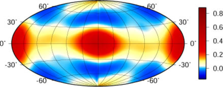
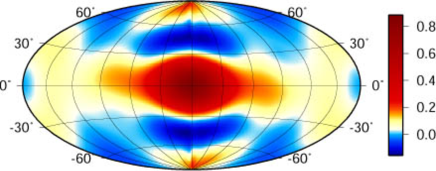
Figure 9: Reconstructed skymap from the time-modulation signals based on the time-series representation. Here, to perform the reconstruction analysis, the number of grid and/or mesh for the discretized data set (33) was specified as $M=16$ in time and $N=17\times 32$ in spherical coordinate. The left panel shows the lowest-order result in which only the $\ell=0$, $2$ and $4$ modes are included, while the right panel represents the result taking account of the leading-order correction to the antenna pattern functions, which includes the multipoles, $\ell\leq 5$.

IV.3.2 Under-determined case

Turning to focus on the analysis based on the harmonic-Fourier representation, we next consider the under-constrained case in which the number of available Fourier components is restricted due to the noises (case A and B discussed in Sec.IV.2). Fig.10 shows the reconstructed images of GWB intensity map in Galactic coordinate, free from the noises but ] restricting the number of Fourier components according to Table 2. The top panel is the intensity map obtained from the lowest-order signals $\mathbf{c}^{(2)}$. Since the accessible Fourier components are basically the same in the lowest-order analysis, the same results are obtained between case A and B. On the other hand, the bottom panels of Fig.10 represent the skymap reconstructed from both $\mathbf{c}^{(2)}$ and $\mathbf{c}^{(3)}$, which indicate that the different images of GWB skymap are obtained depending on the available number of Fourier components (or the amplitude of GWB spectrum); case A (left) and case B (right). In Fig.11, numerical values of the reconstructed multipoles $p_{\ell m}$ in ecliptic coordinate are summarized together with the statistical errors. The statistical errors were roughly estimated according to the discussion in Appendix E based on the SNR [Eq. (38)].

It turns out that the case A fails to reconstruct all the dipole moments, while they can be somehow reproduced in the case B. This is because the cross-correlation data $AT$ and $ET$ which include the information about $\ell=1$ modes were not used in the reconstruction analysis in case A. Although the $\ell=5$ modes of multipole coefficients were not reproduced well in both cases, their contributions to the intensity distribution are not large. Hence, the reconstructed GWB skymap in case B roughly matches the expected intensity map in Fig.4 and the visual impression becomes better than case A. This readily implies that large amplitude of the GWB spectrum is required for a correct reconstruction of a skymap, in practice. However, it should be emphasized that the present reconstruction technique can work well in the under-determined cases. Even in the realistic situation with smaller amplitude of GWB spectrum (case A), the reconstructed skymap including the multipoles $\ell<5$ still shows a disk-like structure, which may provide an important clue to discriminate between the Galactic and the extragalactic GWBs.

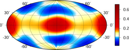
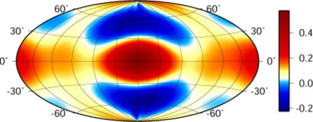
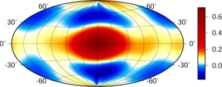
Figure 10: Reconstructed skymap from the time-modulation signals using the restricted Fourier components in under-determined cases (case A, B). These are all plotted in Galactic coordinate. The upper panel shows the result from lowest-order analysis in which only the multipole coefficients of $\ell=0,\,2$ and $4$ modes are considered. The bottom panels are the intensity map taking account of the leading-order correction including the multipoles, $\ell<5$. Left and right panels respectively show the results obtained from the case A and B. Note that the available number of Fourier components was restricted in the reconstruction analysis according to Table 2.

Figure 11: Reconstructed values of the multipole coefficients $|p_{\ell m}|$ in the under-constrained cases. The numerical values are evaluated in the ecliptic coordinates. Left (right) panel shows the result in case A (case B). The open circles with error bar represent the reconstruction results, while the crosses mean the true values. The error bars represent the statistical error in the signal processing. The evaluation of the error is discussed in Appendix E.

V Conclusion and Discussion

In this paper, we have presented a perturbative reconstruction method to make a skymap of GWB observed via space interferometer. The orbital motion of the detector makes the output signals of GWB time-dependent due to the presence of anisotropies of GWB. Since the output signals of GWB are obtained through an all-sky integral of primary signals convolving with an antenna pattern function of gravitational-wave detectors, the time dependence of output data can be used to reconstruct the luminosity distribution of GWBs under full knowledge of detector’s antenna pattern functions. Focusing on the low-frequency regime, we have explicitly given a non-parametric reconstruction method based on both the harmonic-Fourier and the time-series representation. With a help of low-frequency expansion of the antenna pattern functions, the least-squares approximation by SVD enables us to obtain the multipole coefficients of GWB or direct intensity map even when the system becomes over-determined or under-determined. For illustrative purpose, the reconstruction analysis of the GWB skymap has been demonstrated for the confusion-noise background of Galactic binaries around the low-frequency $f=1$mHz. It then turned out that the space interferometer LISA free from the noises is capable of making a skymap of Galactic GWB with angular resolution up to the multipoles, $\ell=5$. For more realistic case based on the estimation of signal-to-noise ratios, the system tends to become under-determined and the number of Fourier components used in reconstruction analysis would be severely restricted. Nevertheless, the resultant skymap still contains the information of the multipoles up to $\ell<5$, from which one can infer that the main sources of GWB come from the Galactic center.

Although the present paper focuses on the reconstruction of the GWB skymap from the LISA, the methodology discussed in Sec.III is quite general and is also applicable to the reconstruction of low-frequency skymap obtained from the ground detectors as well as the other space interferometers, provided their antenna pattern functions. Despite a wide applicability of the present method, however, accessible multipole moments of low-frequency GWB are generally restricted to lower multipoles due to the properties of antenna pattern functions. This would be generally true in any gravitational-wave detectors at the frequencies $f<f_{*}=c/(2\pi L)$, where $L$ is arm-length of single detector or separation between the two detectors. Hence, with the limited angular resolution, only the present methodology may not give a powerful constraint on the luminosity distribution of GWBs. In this respect, we need to combine the other techniques such as the parametric reconstruction method, in which we specifically assume an explicit functional form of the luminosity distribution characterized by the finite number of model parameters and determine them through the likelihood analysis. The data analysis strategy to give a tight constraint on the luminosity distribution is definitely a very important issue and it must be considered urgently. Nevertheless, we note that detectable multipole moments depend practically on the signal-to-noise ratios. Since the signal-to-noise ratios are determined both from the amplitude of GWB and detector’s intrinsic noises, a further feasibility study is necessary in order to clarify the detectable multipole moments correctly. With improved data analysis strategy, it might be even possible that the angular resolution of GWB skymap becomes better than that of LISA considered in the present paper.

Another important issue on the map-making problem is to consider the reconstruction of skymap beyond the low-frequency regime, where the antenna pattern functions give a complicated response to the anisotropic GWBs and thereby the angular resolution of GWB map can be improved Kudoh and Taruya (2005a). Since the low-frequency expansion cannot be used there, a new reconstruction technique should be devised to extract the information of anisotropic GWBs. Further, in the case of LISA, the effect of arm-length variation becomes important and the rigid adiabatic treatment of the detector response cannot be validated. Hence, as emphasized in Sec.III.2, it would become essential to consider the reconstruction method based on the time-series representation, in which no additional assumptions for spacecraft configuration and/or motion are needed to compute the antenna pattern functions. The analysis concerning this issue will be presented elsewhere.

Appendix A Multipole coefficients of antenna pattern functions in low-frequency regime

In this appendix, based on the analytic expression (21) of paper I, the multipole moments for antenna pattern functions of optimal TDIs are calculated at detector’s rest frame. Using the low-frequency approximation $\hat{f}\ll 1$, we present the perturbative expressions up to the forth order in $\hat{f}$.

To evaluate the antenna pattern functions, we must first specify the directional unit vectors $\mathbf{a}$, $\mathbf{b}$ and $\mathbf{c}$, which connect respective spacecrafts. Here, we specifically choose (Fig. 1 and Eq.(28) of Paper I):

$$\mathbf{a}=-\frac{\sqrt{3}}{2}\,\mathbf{x}+\frac{1}{2}\,\mathbf{y},\quad\quad\mathbf{b}=-\mathbf{y},\quad\quad\mathbf{c}=\frac{\sqrt{3}}{2}\,\mathbf{x}+\frac{1}{2}\,\mathbf{y},$$

where the vectors $\mathbf{x}$ and $\mathbf{y}$ respectively denote the unit vectors parallel to the $x$- and $y$-axes in detector’s rest frame (see Fig.1 of Paper I). Then, based on the expression (15), the antenna pattern functions of the optimal TDIs, $\mathcal{F}_{IJ}$ $(I,J=A,E,T)$ are analytically computed at detector’s rest frame. Their multipole moments become

$$a_{\ell m}(\hat{f})=\int_{0}^{\pi}d\theta\,\int_{0}^{2\pi}\,d\phi\,\sin\theta\,\,Y_{\ell m}^{*}(\theta,\phi)\,\,\mathcal{F}(\hat{f},\theta,\phi),$$ (41)

which are expressed as a function of normalized frequency $\hat{f}=f/f_{*}$. Here, for definiteness, we write down the explicit form of the harmonic functions $Y_{\ell m}$:

$$Y_{\ell}^{m}(\theta,\phi)=\sqrt{\frac{2\ell+1}{4\pi}\,\frac{(\ell-m)!}{(\ell+m)!}}\,\,P_{\ell}^{m}(\cos\theta)\,\,e^{im\phi}.$$ (42)

The analytic expressions for the multipole moments $a_{\ell m}$ are generally intractable due to the complicated form of the antenna pattern functions. In the low-frequency regime, however, the perturbative treatment regarding $\hat{f}$ as a small expansion parameter is applied to derive an analytic expression of multipole moments. Below, we summarize the perturbation results up to the fourth order in $\hat{f}$:

$${\mathcal{F}}_{AA}: a_{00}=\frac{2\sqrt{\pi}}{5}\,\hat{f}^{2}-\frac{211\sqrt{\pi}}{1260}\,\hat{f}^{4},\quad a_{20}=\frac{4}{7}\sqrt{\frac{\pi}{5}}\,\hat{f}^{2}-\frac{16}{63}\sqrt{\frac{\pi}{5}}\,\hat{f}^{4}\quad a_{22}=-\frac{1-i\,\sqrt{3}}{756}{\sqrt{\frac{15\pi}{2}}}\,{\hat{f}}^{4},$$ (45)

$$a_{40}=\frac{\sqrt{\pi}}{105}\,{\hat{f}}^{2}+\frac{13\sqrt{\pi}}{9240}\,{\hat{f}}^{4},\quad a_{42}=\frac{13(1-i{\sqrt{3}})}{5544}\sqrt{\frac{\pi}{10}}\,{\hat{f}}^{4},\quad a_{44}=-\frac{1+i\sqrt{3}}{6}\sqrt{\frac{\pi}{70}}\,{\hat{f}}^{2}+\frac{13(1+i\sqrt{3})}{792}\sqrt{\frac{5\pi}{14}}\,{\hat{f}}^{4}$$

$$a_{60}=\frac{1}{1848}\sqrt{\frac{\pi}{13}}\,{\hat{f}}^{4},\qquad a_{62}=-\frac{(1-i\,\sqrt{3})}{4752}\sqrt{\frac{3\pi}{455}}\,{\hat{f}}^{4},\qquad a_{64}=-\frac{1+i\sqrt{3}}{396}\sqrt{\frac{\pi}{182}}\,{\hat{f}}^{4},$$

for self-correlated antenna pattern, $\mathcal{F}_{AA}$. Note that the multipole moments of ${\mathcal{F}}_{EE}$ are related to those of $\mathcal{F}_{AA}$ through the relations, $a_{\ell m}^{\scriptscriptstyle\rm EE}=a_{\ell m}^{\scriptscriptstyle\rm AA}$ for $m=0,\pm 6,\pm 12,\pm 18,\cdots$ and $a_{\ell m}^{\scriptscriptstyle\rm EE}=-a_{\ell m}^{\scriptscriptstyle\rm AA}$ for $m=\pm 2,\pm 4,\pm 8,\cdots$ (see Paper I). The multipole moments of cross-correlation signals are

$${\mathcal{F}}_{AE}: a_{22}=\frac{3+i\sqrt{3}}{756}\sqrt{\frac{5\pi}{2}}\,{\hat{f}}^{4},\quad a_{33}=\frac{1}{18}\sqrt{\frac{7\pi}{15}}\,{\hat{f}}^{3},\quad a_{42}=-\frac{13(\sqrt{3}+i)}{5544}\sqrt{\frac{\pi}{10}}\,{\hat{f}}^{4},\quad$$ (48)

$$a_{44}=\frac{\sqrt{3}-i}{6}\sqrt{\frac{\pi}{70}}\,\hat{f}^{2}-\frac{13(\sqrt{3}-i)}{792}\sqrt{\frac{5\pi}{14}}\,\hat{f}^{4},\quad a_{53}=\frac{1}{18}\sqrt{\frac{\pi}{1155}}\,{\hat{f}}^{3},\quad a_{62}=\frac{\sqrt{3}+i}{4752}\sqrt{\frac{3\pi}{455}}\,{\hat{f}}^{4},$$

$$a_{64}=\frac{\sqrt{3}-i}{396}\sqrt{\frac{\pi}{182}}\,{\hat{f}}^{4},$$

$${\mathcal{F}}_{AT}: a_{11}=\frac{(1+i\sqrt{3})\sqrt{\pi}}{168}\,{\hat{f}}^{3},\quad a_{22}=-\frac{\sqrt{3}+i}{864}\sqrt{\frac{3\pi}{5}}\,{\hat{f}}^{4},\quad a_{31}=\frac{1+i\sqrt{3}}{72}{\sqrt{\frac{\pi}{14}}}\,{\hat{f}}^{3},\quad$$ (51)

$$a_{42}=\frac{\sqrt{3}+i}{3168}{\sqrt{\frac{\pi}{5}}}\,{\hat{f}}^{4},\quad a_{44}=\frac{17(\sqrt{3}-i)}{3168}\sqrt{\frac{\pi}{35}}\,{\hat{f}}^{4},\quad a_{51}=\frac{1+i\sqrt{3}}{1008}{\sqrt{\frac{\pi}{55}}}\,{\hat{f}}^{3},$$

$$a_{55}=\frac{1-i\sqrt{3}}{72}{\sqrt{\frac{3\pi}{154}}}\,{\hat{f}}^{3},\quad a_{62}=\frac{\sqrt{3}+i}{4752}{\sqrt{\frac{3\pi}{910}}}\,{\hat{f}}^{4},\quad a_{64}=\frac{\sqrt{3}-i}{3168}{\sqrt{\frac{\pi}{91}}}\,{\hat{f}}^{4}.$$

The multipole moments of antenna pattern function $\mathcal{F}_{ET}$ are also obtained from those of $\mathcal{F}_{AT}$ using the relation, $a_{\ell m}^{ET}=-(i/\sqrt{3})\,\tan\left(m\pi/3\right)a_{\ell m}^{AT}$, as shown in Paper I.

Finally, we also list the multipole moments of self-correlated antenna pattern $\mathcal{F}_{TT}$, which are all higher-order contribution with $\mathcal{O}(\hat{f}^{4})$:

$${\mathcal{F}}_{TT}: a_{00}=\frac{\sqrt{\pi}}{504}\,{\hat{f}}^{4},\qquad a_{40}=-\frac{\sqrt{\pi}}{1584}\,{\hat{f}}^{4},\qquad a_{60}=-\frac{1}{11088}\sqrt{\frac{\pi}{13}}\,{\hat{f}}^{4},\qquad a_{66}=-\frac{1}{48}\sqrt{\frac{\pi}{3003}}\,{\hat{f}}^{4}.$$ (52)

Appendix B Remarks on the degeneracy between monopole and quadrupole moments for LISA measurement of GWB anisotropy

The reconstruction method based on the harmonic-Fourier representation (14) presented in Sec.III.1 has been first discussed by Cornish Cornish (2001, 2002a). Later, Seto & Cooray Seto and Cooray (2004) considered the reconstruction of a skymap in the low-frequency limit using the optimal set of TDI signals $A$ and $E$. In this case, the accessible multipole moments $p_{\ell m}$ are $\ell=0,\,2$ and $4$ (see Table 1). Seto & Cooray explicitly wrote down the expressions for linear equation (14) in the case of the self-correlation signals (i.e., AA-, EE-correlations) and showed that the output data with sufficient statistical significance are only $\widetilde{C}_{0}$, $\widetilde{C}_{\pm 1}$ and $\widetilde{C}_{\pm 2}$. Further, they found that the multipole coefficients $p_{00}$ and $p_{20}$ cannot be separately determined due to the degeneracy associated with a specific combination between the Wigner $D$ matrices and the antenna pattern functions.

Here, we explicitly point out the origin of this degeneracy and discuss its influences on the reconstruction of GWB skymap. Using the multipole coefficients of antenna patterns in Appendix A, the lowest-order contribution to the linear system (14) for AA- and EE-correlations becomes

$$\widetilde{C}^{(2)}_{AA,0} = \frac{1}{4\sqrt{\pi}}\left\{\frac{2}{5}\,p_{00}-\frac{1}{14\sqrt{5}}\,p_{20}-\frac{37}{13440}\,p_{40}-\frac{27}{512\sqrt{70}}\sum_{m=-4,4}b_{4m}^{\scriptscriptstyle({\mathrm{AA}})}\,p_{4m}\right\},$$ (53)

$$\widetilde{C}^{(2)}_{EE,0} = \frac{1}{4\sqrt{\pi}}\left\{\frac{2}{5}\,p_{00}-\frac{1}{14\sqrt{5}}\,p_{20}-\frac{37}{13440}\,p_{40}+\frac{27}{512\sqrt{70}}\sum_{m=-4,4}b_{4m}^{\scriptscriptstyle({\mathrm{AA}})}\,p_{4m}\right\}.$$ (54)

with $b^{\scriptscriptstyle({\mathrm{AA}})}_{44}=1-i\sqrt{3}=[b^{\scriptscriptstyle({\mathrm{AA}})}_{4,-4}]^{*}$. Here, we only show the relevant components of $\widetilde{C}_{k}$ which contains the multipole coefficients $p_{00}$ and $p_{20}$. The above expressions include the multipole coefficients of $\ell=4$, which are all determined separately from the lowest-order contribution of $AE$-correlation, $\widetilde{C}_{AE,k}^{(2)}$. Thus, apart from the octupole moments, equations (53) and (54) clearly show the presence of degeneracy between the remaining multipole coefficients, $p_{00}$ and $p_{20}$.

In a language of the least-squares method by SVD, this degeneracy implies that the sub-system in the matrix equation (31) containing the coefficients $p_{00}$ and $p_{20}$ becomes under-determined. In this case, the least-squares method by SVD cannot correctly produce the approximate solutions for $p_{00}$ and $p_{20}$, although it still provides some “approximate” solution. From equations (53) and (54), the only meaningful equation for $p_{00}$ and $p_{20}$ is now reduced to

$$\widetilde{C}=\frac{1}{4\sqrt{\pi}}\left(\frac{2}{5}\,p_{00}-\frac{1}{14\sqrt{5}}\,p_{20}\right),$$ (55)

where the numerical constant $\widetilde{C}$ represents a collection of the irrelevant terms of $\ell=4$ modes, which are separately determined from the linear system in $AE$-correlation. If one naively applies the least-squares method to the above system, a very tight relation is obtained:

$$p_{00}=\frac{7840\sqrt{\pi}}{789}\,\,\widetilde{C},\quad\quad p_{20}=\frac{280\sqrt{5\pi}}{789}\,\,\widetilde{C}.$$ (56)

The presence of degenerate coefficients may be a big obstacle in constructing the skymap as well as in determining the normalization factor of GWB spectrum. In principle, this degeneracy can be broken when we consider the higher-order terms of $\mathcal{O}(\hat{f}^{4})$. However, these terms are generally small and irrelevant for the reconstruction analysis in the low-frequency regime. In this sense, the reconstruction of low-frequency skymap is, in nature, incomplete and the other additional information for monopole or quadrupole moment is required to make a full skymap. Nevertheless, it should be emphasized that with a high signal-to-noise ratio, the other remaining multipole coefficients can be all determined by the least-squares solution by SVD, independently of the above degeneracy. Moreover, in cases with $p_{00}\gg p_{20}$, which is usually satisfied, the least-squares solution (56) provides a modest estimate of the degenerate coefficients $p_{00}$ and $p_{20}$ because of the hierarchy of the coefficients in Eq. (56). This point has been explicitly demonstrated in Sec.IV.

Appendix C Data sets and least-squares method

In this appendix, we describe in more details how to obtain the multipole moments of GWBs from many data streams by applying the least-squares method. Here we specifically focus on the situation considered in Sec. IV.3.1. That is, the data sets that we use are (i) the $k=-2\sim+2$ components of self-correlation signals $AA$ and $EE$, (ii) $k=-8\sim+8$ components of $AE$-signal, and (iii) the $k=-4\sim+4$ components of cross-correlation signals $AT$ and $ET$. According to the general strategy given in Sec. III.1 (see Eq. (31)), we first combine the leading data streams of (i) and (ii) which correspond to $i=2$ in Eq. (30). The combined data sets consist of the following matrices.

$$\left(\begin{array}[]{c}\tilde{C}_{+2,AA}^{(2)}\\ \tilde{C}_{+1,AA}^{(2)}\\ \tilde{C}_{-1,AA}^{(2)}\\ \tilde{C}_{-2,AA}^{(2)}\\ \tilde{C}_{+2,EE}^{(2)}\\ \vdots\\ \tilde{C}_{-2,EE}^{(2)}\\ \end{array}\right)=\left(\begin{array}[]{ccccccccccccc}0&0&0&*&\\ 0&0&*&0&\\ 0&*&0&0&\\ &0&0&0&\\ 0&0&0&*&\\ 0&0&*&0&\\ 0&*&0&0&\\ &0&0&0&\\ \end{array}\right)\left(\begin{array}[]{c}p_{22}\\ p_{21}\\ p_{2,-1}\\ p_{2,-2}\\ \end{array}\right),\quad\left(\begin{array}[]{c}\tilde{C}_{+8,AE}^{(2)}\\ \tilde{C}_{+7,AE}^{(2)}\\ \vdots\\ \tilde{C}_{0,AE}^{(2)}\\ \vdots\\ \tilde{C}_{-7,AE}^{(2)}\\ \tilde{C}_{-8,AE}^{(2)}\\ \end{array}\right)=\left(\begin{array}[]{ccccccccccccc}0&&&&*&\\ &&&\rotatebox[origin={c}]{-45.0}{\vdots}&&\\ &\rotatebox[origin={c}]{-45.0}{\vdots}&&&&\\ &&&&*&\\ &&&\rotatebox[origin={c}]{-45.0}{\vdots}&&\\ &\rotatebox[origin={c}]{-45.0}{\vdots}&&&&\\ &&&&0&\\ \end{array}\right)\left(\begin{array}[]{c}p_{44}\\ p_{43}\\ \vdots\\ p_{40}\\ \vdots\\ p_{4,-3}\\ p_{4,-4}\\ \end{array}\right),$$ (57)

where $*$ represents a non-vanishing complex number. Note that for simplicity we have not included the data $\tilde{C}_{0,AA}^{(2)}$ and $\tilde{C}_{0,EE}^{(2)}$, which contain degeneracy between the multipole moments (see Sec. B). The matrices in the right hand side correspond to $\mathbf{A}^{(i)}$ in Eq. (30). These sparse forms of matrix are typical for the present problem. We perform the singular value decomposition with respect to these sparse matrices, and construct pseudo-inverse matrices which give the least-squares solutions of $p_{\ell m}$. In a similar way the least-squares solutions of $\ell=\mathrm{odd}$ modes are obtained from the following matrix equation,

$$\left(\begin{array}[]{c}\tilde{C}_{+8,AE}^{(3)}\\ \vdots\\ \tilde{C}_{-8,AE}^{(3)}\\ \tilde{C}_{4,AT}^{(3)}\\ \vdots\\ \tilde{C}_{-4,AT}^{(3)}\\ \tilde{C}_{4,ET}^{(3)}\\ \vdots\\ \tilde{C}_{-4,ET}^{(3)}\\ \end{array}\right)=\left(\begin{array}[]{ccccccccccccc}&&&&\\ &&\mathbf{A}_{\mathrm{AE}}^{(3)}&&\\ &&&&\\ &&\mathbf{A}_{\mathrm{AT}}^{(3)}&&\\ &&&&\\ &&\mathbf{A}_{\mathrm{ET}}^{(3)}&&\\ &&&&\\ \end{array}\right)\left(\begin{array}[]{c}p_{11}\\ p_{10}\\ p_{1,-1}\\ p_{33}\\ \vdots\\ p_{3,-3}\\ p_{55}\\ \vdots\\ p_{5,-5}\\ \end{array}\right),$$ (58)

where we have symbolically written the matrix ${\mathbf{A}}^{(3)}$ due to space limitation.

Appendix D Multipole coefficients for gravitational-wave backgrounds

Here, we give the multipole coefficients for normalized intensity distribution $P(\mathbf{\Omega})$ of galactic GWB presented in Sec.IV.1. To evaluate this, we first create the intensity map $P(\mathbf{\Omega})$ with $129\times 256$ regular grids of celestial sphere $(\theta,\,\phi)$. Then, the spherical harmonic expansion of the intensity map is numerically carried out using the SPHEREPACK 3.1 package Adams and Swarztrauber (2003). Table 3 summarizes the multipole coefficients $p_{\ell m}$ up to $\ell=5$, which are relevant to the analysis in Sec.IV. Note also that $p_{\ell,-m}=(-1)^{m}p_{\ell m}^{*}$.

To characterize the contribution of the $\ell$-th moment to the galactic GWB, we introduce the angular power defined by

$$\sigma_{\ell}=\left\{\frac{1}{2\ell+1}\,\,\sum_{m=-\ell}^{\ell}|p_{\ell m}|^{2}\right\}^{1/2},$$ (59)

which is rotationally invariant Kudoh and Taruya (2005a). Figure 12 shows the normalized angular power, $\sigma_{\ell}/\sigma_{0}$ up to $\ell=30$. The dominant contribution to the intensity of galactic GWB comes from the multipoles with $\ell\lesssim 4$, however, the asymptotic behavior at higher multipoles is very slow and can be fitted by $\sigma_{\ell}/\sigma_{0}\sim 1.85\,e^{-0.005\ell}/\ell$ (dotted line in Fig.12), which turns out to be a good approximation even to much higher multipoles, $\ell\sim 100$.

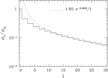
Figure 12: Normalized angular power of galactic GWB anisotropy, $\sigma_{\ell}/\sigma_{0}$ as a function of multipole $\ell$.

Table 3: Multipole coefficients for galactic GWB. $p_{\ell m}$ with $m<0$ is given by $p_{\ell m}=(-1)^{m}p^{*}_{\ell,-m}$.

$\ell$	$m$	Re[$p_{\ell m}$]	Im[$p_{\ell m}$]
0	0	0.282	0
1	0	-0.0215	0
1	1	0.00876	-0.156
2	0	-0.0681	0
2	1	-0.0828	0.0216
2	2	-0.180	-0.0124
3	0	0.0231	0
3	1	0.00419	0.0648
3	2	0.0212	0.0544
3	3	-0.0170	0.135
4	0	0.0120	0
4	1	-0.0205	-0.0224
4	2	0.0807	-0.00274
4	3	0.0936	-0.0198
4	4	0.139	0.0194
5	0	-0.0172	0
5	1	0.000230	-0.0272
5	2	-0.0250	-0.00640
5	3	-0.00336	-0.0693
5	4	-0.0177	-0.0719
5	5	0.0222	-0.1.13

Appendix E Estimation of statistical error in reconstruction analysis

In the reconstruction analysis based on the harmonic-Fourier representation, the statistical errors plotted in Fig.11 are roughly estimated as follows. In the presence of the noises, the least-squares solution given in equation (32) becomes

$$\mathbf{p}^{(i)}_{\rm approx}=\left[\mathbf{A}^{(i)}\right]^{+}\cdot\left\{\mathbf{c}^{(i)}+\mathbf{s}_{\rm n}^{(i)}\right\},$$ (60)

where the additional term $\mathbf{s}_{\rm n}^{(i)}$ represents the noise contributions to the $i$-th order coefficient of perturbative expansion for $\mathbf{c}(f)$. The root-mean-square amplitude of the error $\Delta\mathbf{p}^{(i)}$ is then defined by taking the ensemble average of the random noises as $\Delta\mathbf{p}^{(i)}\equiv\left\langle|\mathbf{p}^{(i)}-\langle\mathbf{p}^{(i)}\rangle|^{2}\right\rangle$, which gives the errors in multipole coefficient $\Delta p_{\ell m}$. The $j$-th components of the vector $\Delta\mathbf{p}^{(i)}$ becomes

$$|\Delta\mathbf{p}^{(i)}_{{\rm approx},j}|^{2}=\left[\mathbf{A}^{(i)}\right]^{+}_{jk}\left[\mathbf{A}^{(i)}\right]^{+*}_{jk}\,\langle|\mathbf{s}_{{\rm n},k}^{(i)}|^{2}\rangle.$$ (61)

Here, the variance $\langle|\mathbf{s}_{\rm n,k}^{(i)}|^{2}\rangle$ roughly corresponds to the quadrature of the vector $\mathbf{c}^{(i)}$ divided by the signal-to-noise ratio:

$$\mathbf{S}_{{\rm n},k}^{(i)}=\left\{\alpha\,\,\frac{\displaystyle\mathbf{c}_{k}^{(i)}}{\displaystyle\mathbf{(s/r)}_{k}}\right\}^{2}.$$ (62)

In the above expression, the vector $\mathbf{(s/r)}$ represents the SNR, each component of which is the quantity $(S/N)_{k}$ defined in (38) just for the same component of the vector $\mathbf{c}^{(i)}$. Notice that the factor $\alpha$ is multiplied in equation (62) by hand. The reason why we have introduced the factor $\alpha$ is as follows. First note that the quantity $(S/N)_{k}$ basically reflects the signal-to-noise ratio for the most dominant term in the perturbative expansion for the signal $\tilde{C}_{k}(f)$ (see Eq.(30)). For the $AE$-correlation, $(S/N)_{k}$ gives the signal-to-noise ratio for second-order term, i.e., $\mathbf{c}^{(2)}$. For the $AT$-correlation, $(S/N)_{k}$ reflects the signal-to-noise ratio for $\mathbf{c}^{(3)}$. In our reconstruction analysis, the higher-order contributions to the $AE$-correlation, $\mathbf{c}^{(3)}$ is used to make the skymap with multipoles $\ell\leq 5$, which can be estimated by analyzing the multi-frequency data. In general, the signal from higher-order contribution is weaker than the lowest-order term, leading to the calibration error. The significance of this error would be enhanced by the factor roughly proportional to $\hat{f}^{-(i-2)}$ for the $i$-th order terms of $AE$-correlation. Hence, in order to mimic this, the factor $\alpha$ is multiplied and set to $\alpha=\hat{f}^{-(i-2)}$. In the case examined in Fig.11, we adopt $\alpha=\hat{f}^{-1}=10$ for third-order cross-correlation data $\tilde{C}_{{\rm AE},k}^{(3)}$. Otherwise we set $\alpha=1$. As a result, statistical errors of $\ell=3$ modes become larger than those in $\ell=$even modes (see Fig.11). Note that the multipole coefficients with $\ell=1$ in case A and with $\ell=5$ in both case are completely degenerate and cannot be recovered by reconstruction analysis. Hence, the statistical errors were not evaluated.

Appendix F Computational method of multipole coefficients

In this Appendix, we give a brief description of the numerics of calculating the multipole coefficients using the SPHEREPACK 3.1 package Adams and Swarztrauber (2003). The traditional spherical harmonic transform of a scalar function is

$$\Psi(\theta,\phi)=\sum_{\ell,m}p_{\ell m}Y_{\ell m}(\theta,\phi).$$ (63)

The spherical harmonics are given by equation (42) and the associated Legendre polynomials are

$$P^{m}_{\ell}(x)=\frac{(-1)^{m}}{2^{\ell}\ell!}(1-x^{2})^{m/2}\frac{d^{m+\ell}}{dx^{m+\ell}}(x^{2}-1)^{\ell}.$$ (64)

On the other hand, numerical computation of spherical harmonic expansion is performed with the subroutine shaec in SPHEREPACK 3.1 package, which directly gives the following expansion form:

$$\Psi(\theta,\phi) = \sqrt{\frac{\pi}{2}}\sum_{\ell=0}^{\infty}\sum_{m=0}^{\infty}{}^{\prime}P^{m}_{\ell}(\cos\theta)\gamma_{\ell m}\left[\alpha_{\ell m}\cos m\phi-\beta_{\ell m}\sin m\phi\right],$$ (65)

where the prime notation on the sum indicates that the first term corresponding to $m=0$ is multiplied by the factor $1/2$. To relate the coefficients $\alpha_{\ell m}$ and $\beta_{\ell m}$ with $p_{\ell m}$, the expansion (63) is compared with the expression (65), leading to

$$p_{\ell m} = \sqrt{\frac{\pi}{2}}(\alpha_{\ell m}+i\beta_{\ell m}),$$ (66)

$$(-1)^{m}p_{\ell,-m} = \sqrt{\frac{\pi}{2}}(\alpha_{\ell m}-i\beta_{\ell m}),$$ (67)

for $m>0$, and

$$p_{\ell 0}=\sqrt{\frac{\pi}{2}}\alpha_{\ell 0},$$ (68)

for $m=0$. Hence, with a help of these expressions, one can read off the multipole coefficients $p_{\ell m}$ from the expansion formula (65). Notice that the associated Legendre polynomials used in the SPHEREPACK 3.1 package differ from (64) by a factor $(-1)^{m}$ so that one must multiply this factor to the transformation law (67) and (68).

References

- Seto et al. (2001) N. Seto, S. Kawamura, and T. Nakamura, Phys. Rev. Lett. 87, 221103 (2001), eprint astro-ph/0108011.
- BBO (2003) URL, http://universe.gsfc.nasa.gov/program/bbo.html (2003).
- Ungarelli and Vecchio (2001a) C. Ungarelli and A. Vecchio, Phys. Rev. D63, 064030 (2001a), eprint gr-qc/0003021.
- Smith et al. (2005) T. L. Smith, M. Kamionkowski, and A. Cooray (2005), eprint astro-ph/0506422.
- Hils et al. (1990) D. Hils, P. L. Bender, and R. F. Webbink, Astrophys. J. 360, 75 (1990).
- Bender and Hils (1997) P. L. Bender and D. Hils, Class. Quant. Grav. 14, 1439 (1997).
- Nelemans et al. (2001) G. Nelemans, L. R. Yungelson, and S. F. Portegies Zwart, Astron. Astrophys. 375, 890 (2001), eprint astro-ph/0105221.
- Benacquista et al. (2004) M. J. Benacquista, J. DeGoes, and D. Lunder, Class. Quant. Grav. 21, S509 (2004), eprint gr-qc/0308041.
- Edlund et al. (2005) J. A. Edlund, M. Tinto, A. Krolak, and G. Nelemans, Phys. Rev. D71, 122003 (2005), eprint gr-qc/0504112.
- Timpano et al. (2005) S. E. Timpano, L. J. Rubbo, and N. J. Cornish (2005), eprint gr-qc/0504071.
- Giampieri and Polnarev (1997a) G. Giampieri and A. G. Polnarev, Mon. Not. R. Astron. Soc. 291, 149 (1997a).
- Giampieri and Polnarev (1997b) G. Giampieri and A. G. Polnarev, Class. Quant. Grav. 14, 1521 (1997b).
- Allen and Ottewill (1997) B. Allen and A. C. Ottewill, Phys. Rev. D56, 545 (1997), eprint gr-qc/9607068.
- Ungarelli and Vecchio (2001b) C. Ungarelli and A. Vecchio, Phys. Rev. D64, 121501 (2001b), eprint astro-ph/0106538.
- Cornish (2001) N. J. Cornish, Class. Quant. Grav. 18, 4277 (2001), eprint astro-ph/0105374.
- Cornish (2002a) N. J. Cornish, Class. Quant. Grav. 19, 1279 (2002a).
- Seto (2004) N. Seto, Phys. Rev. D69, 123005 (2004), eprint gr-qc/0403014.
- Seto and Cooray (2004) N. Seto and A. Cooray (2004), eprint astro-ph/0403259.
- Kudoh and Taruya (2005a) H. Kudoh and A. Taruya, Phys. Rev. D71, 024025 (2005a), eprint gr-qc/0411017.
- Cutler (1998) C. Cutler, Phys. Rev. D57, 7089 (1998), eprint gr-qc/9703068.
- Moore and Hellings (2002) T. A. Moore and R. W. Hellings, Phys. Rev. D65, 062001 (2002), eprint gr-qc/9910116.
- Peterseim et al. (1997) M. Peterseim, O. Jennrich, K. Danzmann, and B. F. Schutz, Class. Quant. Grav. 14, 1507 (1997).
- Takahashi and Nakamura (2003) R. Takahashi and T. Nakamura, Astrophys. J. 596, L231 (2003), eprint astro-ph/0307390.
- Edmonds (1957) A. R. Edmonds, Angular Momentum in Quantum Mechanics Princeton University Press p. 59 (1957).
- Prince et al. (2002) T. A. Prince, M. Tinto, S. L. Larson, and J. W. Armstrong, Phys. Rev. D66, 122002 (2002), eprint gr-qc/0209039.
- Nayak et al. (2003) K. R. Nayak, A. Pai, S. V. Dhurandhar, and J.-Y. Vinet, Class. Quant. Grav. 20, 1217 (2003), eprint gr-qc/0210014.
- Cornish (2002b) N. J. Cornish, Phys. Rev. D65, 022004 (2002b), eprint gr-qc/0106058.
- Armstrong et al. (1999) J. W. Armstrong, F. B. Estabrook, and M. Tinto, Astrophys. J. 527, 814 (1999).
- Krolak et al. (2004) A. Krolak, M. Tinto, and M. Vallisneri (2004), eprint gr-qc/0401108.
- Press et al. (2002) W. H. Press, S. A. Teukolsky, W. T. Vetterling, and B. P. Flannery, Numerical Recipes in C++ (Cambridge University Press) (2002).
- Cornish and Hellings (2003) N. J. Cornish and R. W. Hellings, Class. Quant. Grav. 20, 4851 (2003), eprint gr-qc/0306096.
- Tinto et al. (2004) M. Tinto, F. B. Estabrook, and J. W. Armstrong, Phys. Rev. D69, 082001 (2004), eprint gr-qc/0310017.
- Shaddock (2004) D. A. Shaddock, Phys. Rev. D69, 022001 (2004), eprint gr-qc/0306125.
- Binney et al. (1997) J. Binney, O. Gerhard, and D. Spergel, Mon. Not. R. Astron. Soc. 288, 365 (1997), eprint astro-ph/9609066.
- Adams and Swarztrauber (2003) J. C. Adams and P. N. Swarztrauber, http://www.scd.ucar.edu/css/software/spherepack/ (2003).
- Kudoh and Taruya (2005b) H. Kudoh and A. Taruya (2005b), eprint in preparation.
- Bender and et. al., (1998) P. L. Bender and et. al.,, LISA Pre-Phase A Report (1998).