A Toy Model for Testing Finite Element Methods to Simulate Extreme-Mass-Ratio Binary Systems

Abstract

Extreme mass ratio binary systems, binaries involving stellar mass objects orbiting massive black holes, are considered to be a primary source of gravitational radiation to be detected by the space-based interferometer LISA. The numerical modelling of these binary systems is extremely challenging because the scales involved expand over several orders of magnitude. One needs to handle large wavelength scales comparable to the size of the massive black hole and, at the same time, to resolve the scales in the vicinity of the small companion where radiation reaction effects play a crucial role. Adaptive finite element methods, in which quantitative control of errors is achieved automatically by finite element mesh adaptivity based on posteriori error estimation, are a natural choice that has great potential for achieving the high level of adaptivity required in these simulations. To demonstrate this, we present the results of simulations of a toy model, consisting of a point-like source orbiting a black hole under the action of a scalar gravitational field.

I Introduction

As we enter the era of Gravitational Wave Astronomy, a number of experiments to detect and study gravitational waves have been set up and some others are presently under development (see Hough et al. (2005) for a recent account). Among the second group we find one of the experiments that is presently attracting a considerable amount of attention: the Laser Interferometer Space Antenna (LISA) Vitale et al. (2002); Danzmann (2003); Danzmann and Rudiger (2003); Prince (2003), a collaboration between ESA and NASA that is scheduled to be launched in the next decade. Extreme-Mass-Ratio Binaries (EMRBs) are considered to be a primary source of gravitational radiation to be detected by LISA Barack and Cutler (2004); Gair et al. (2004). They consist of a “small” object, such a main sequence star, a stellar mass black hole, or a neutron star, with mass $m$ ranging from $1M_{\odot}$ to $10^{2}M_{\odot}$, orbiting a massive black hole (MBH) with mass $M$ ranging from $10^{3}M_{\odot}$ (if we consider the case of intermediate mass black holes) to $10^{9}M_{\odot}$ (the case of big supermassive black holes sitting in the center of galaxies). This translates to EMRBs with mass ratios, $\mu=m/M\,,$ in the range $10^{-3}-10^{-9}\,$. In order to exploit this type of systems through LISA, it is crucial to have a good theoretical understanding of the evolution of these systems, good enough to produce accurate waveform templates in support of data analysis efforts.

Because there is no significant coupling between the strong curvature effects between the MBH and its companion, relativistic perturbation theory is a well suited tool to study EMBRs. Clearly, the accuracy of this approximation depends on the smallness of the ratio $\mu$. The goal is to study the perturbations generated by the small body in the (background) gravitational field of the MBH, and how these perturbations affect the motion of the small body itself, which follows the geodesics of the perturbed spacetime. That is, one is after studying how the presence of the small body affects its own trajectory. This problem is usually known in literature as the radiation reaction problem. This is an old problem and several approaches to deal with it have been proposed (see the recent reviews by Poisson Poisson (2004, 2005), Detweiler Detweiler (2005) and Mino Mino (2005a, b, c)). A pragmatic approach is to use energy-momentum balance arguments Tanaka et al. (1993); Cutler et al. (1994); Hughes (2000, 2001a, 2001b); Glampedakis et al. (2002). Under this approach, one estimates the changes in the small body constants of motion by computing the fluxes of energy and angular momentum at infinity and through the MBH horizon. This approach works well in the adiabatic regime, when the time scale of the radiation reaction is much bigger than the orbital time scale. Until now it has dealt with special orbits of the Kerr black hole, but it has not yet produced results for generic orbits because of the difficulty of adjusting the third constant of motion, the Carter constant, present in generic geodesics of the Kerr spacetime. However, there have been some recent advances in this direction Mino (2003); Hughes et al. (2005); Drasco et al. (2005); Sago et al. (2005).

An alternative approach consists in trying to describe the radiation reaction effects on the small body as the action of a local self-force that is responsible for the deviations from the geodesic motion. A rigorous formulation of this concept has been given by the first time by Mino, Sasaki and Tanaka Mino et al. (1997), and later, adopting an axiomatic approach, by Quinn and Wald Quinn and Wald (1997). These works give a formal prescription to compute the self-force. For the practical implementation of these prescription some techniques have been proposed (see Lousto (2005) for a recent progress report): the mode-sum scheme Barack and Ori (2000); Barack (2000, 2001); Barack et al. (2002), and a regularization scheme based on zeta-function regularization techniques Lousto (2000).

In this paper we want to advocate an alternative, and at the same time complementary, approach: The direct numerical integration of the (linearized) evolution equations for the gravitational field together with the evolution equations for the small body, which form a system of partial differential equations (PDEs) coupled to a system of ordinary differential equations (ODEs). We can already find in the literature an attempt to use numerical methods for simulating EMRBs Bishop et al. (2003). In this work, the perturbations are computed by using the full general relativistic equations in the framework of the characteristic formulation (in contrast to a Cauchy-type formulation), with the small body being described by an energy-momentum distribution that moves “rigidly” along a geodesic of the numerically computed spacetime. The main drawback of this work is the size of the small body, which is bigger than the MBH horizon. Another approach that has been used in the literature Lopez-Aleman et al. (2003) is to describe the gravitational field by using the Teukolsky formalism Teukolsky (1973) implemented in the time domain (using a numerical code introduced in Krivan et al. (1997)) and by modelling the small body by smearing the singularities in the source term by the use of narrow Gaussian distributions. This work has also the problem that the size of the small body is too big (in comparison with the size of the MBH). This shows the main underlying difficulty in the numerical simulation of EMRBs, namely, the problem involves a vast range of physical scales (spatial and temporal) that expand over several orders of magnitude. Specifically, one needs to handle not only large wavelength scales comparable to the massive black hole, but also to resolve the scales in the vicinity of the small object where radiation reaction effects play a crucial role.

An obvious conclusion we can extract from these facts is that, in order to carry out successful numerical simulations of EMRBs, we need a high degree of adaptivity. Our proposal is the use of the Finite Element Method (FEM) as a natural choice to achieve this high level of adaptivity. Finite Element Methods have not been used occasionally in General Relativity (see Arnold et al. (1998); Metzger (2004)) To demonstrate that these numerical techniques have great potential of leading to successful simulations of EMRBs, we present results from simulations of a toy problem consisting of a point-like source orbiting a black hole in scalar gravitation in $2+1$ dimensions. Our aim is to test FEM techniques in a simple representative problem that possesses the main ingredients and challenges of the astrophysical EMRBs. That is, at this stage we are basically conducting a feasibility study. In our toy model, the spacetime metric is fixed and aims at describing the gravitational field of a non-rotating black hole. For computational efficiency, we have made a reduction from three spatial dimensions to two. In this reduction, which we explain in detail later, the metric we work with is not longer a solution of the Einstein vacuum equations but it keeps the important property that its geodesics coincide with the equatorial geodesics of the Schwarzschild spacetime. This metric is not dynamical but fixed. The dynamical gravitational field is described by a scalar field on this spacetime, satisfying a wave-like equation with a source term that describes the presence of the small object. An important ingredient of our model is the use of a particle description for the small object. The equations of motion of this particle are the geodesics of the fixed spacetime metric modified by the presence of (spatial) components of the gradient of the gravitational scalar field. In this way we have that the particle orbits the black hole subject to radiation reaction: indeed, the particle generates the scalar gravitational field which affects its own motion.

In this work we compare numerical simulations that use the simple classical FEM with simulations that use an adaptive-mesh FEM. The essence of the adaptive mesh technique is to produce real-time local mesh coarsening or refinement to achieve the desired level of smoothness in the solution. To that end, a good posteriori error estimator to predict the regions in the computational domain where rapidly changes take place is extremely important. There are several ways to approach this problem. Theoretical research on this subject Chen et al. (2003) has found that the Hessian matrix of the numerical solution can accurately predict where the steepest gradients of the solution would take place. We demonstrate that this technique when applied to our toy model easily captures the dynamics of the field in the vicinity of the particle since around the particle location either the field or the source term will change much more than anywhere else. We then refine the local area surrounding the particle and resolve it more accurately so that we are able to achieve our final target.

The plan of this paper is the following: In Section II we introduce the particular theoretical model we want to study, namely: the description of the gravitational field and of the point-like source, the computational setup, and an energy balance test that can be used to test the numerical computations. In Section III we describe the computational techniques that we use for the time-domain simulations of our theoretical model: the FEM, the discretization of our equations using Finite Elements, the numerical method for solving the equations of motion of the particle, and finally, the Adaptive Finite Element Method (AFEM). In Section IV we present and discuss the numerical results of the simulations. Here, we distinguish between the simulations that use the classical FEM and those that use the AFEM. We devote the last Section V to discuss the main results of this work and the future perspectives that it opens.

II Theoretical aspects of the toy model

In the following, we describe in detail the main aspects of our toy model, namely: (i) the gravitational theory we use, (ii) the derivation of the equations to be solved, (iii) the particle’s description, and (iv) the computational setup. We use physical units in which $c=G=1\,.$ We use lowercase Greek letters for spacetime indices and lowercase Latin letters for spatial indices. In subsections II.1 and II.2 indices run as: $\mu\,,\nu\,,\ldots=0-3\,;$ $i\,,j\,,\ldots=1-3\,.$

II.1 Scalar Gravity

Scalar gravitation is a theory of gravity that although it cannot we applied to our physical world (we know it cannot fit all the available experimental data), is a good laboratory for numerical relativity due to its simplicity. Of particular interest for our purposes is the fact that (scalar) gravitational waves exist in scalar gravity. In this theory, the gravitational field is described by a scalar field $\Phi(x^{\mu})$ on a spacetime geometry described by a non-dynamical metric tensor $\mbox{g}_{\mu\nu}$, which we just prescribe (the version presented in problem 7.1 of the textbook by Misner, Thorne and Wheeler Misner et al. (1973) and in Shapiro and Teukolsky (1993, 1994); Scheel et al. (1994) considers only the case in which the non-dynamical spacetime is the flat spacetime). The scalar field does not affect to the spacetime structure defined by $\mbox{g}_{\mu\nu}$. We are interested in studying the evolution of a particle-like object orbiting a black hole in this theory. To that end, we consider a background spacetime metric $\mbox{g}_{\mu\nu}$ describing the geometry of a non-rotating black hole, and a particle of mass $m$ that follows the worldline $z^{\mu}(\tau)$, where $\tau$ denotes the particle proper time. The action of this particle-field system is

$$S=\int\sqrt{-g}{\cal L}d^{4}x=-\int\sqrt{-g}\left(\frac{1}{8\pi}\mbox{g}^{\mu\nu}\nabla_{\mu}\Phi\nabla_{\nu}\Phi-\rho\mbox{e}^{\Phi}\right)d^{4}x\,,$$ (1)

where the comoving density $\rho$, describing the particle, is given by

$$\rho=\int\frac{m}{\sqrt{-g}}\delta^{4}[x^{\mu}-z^{\mu}(\tau)]d\tau=\frac{m}{u^{t}\sqrt{-g}}\delta^{3}[x^{i}-z^{i}(t)]\,,$$ (2)

where $t$ is a time coordinate and $u^{t}$ is the corresponding component of the velocity of the particle:

$$u^{\mu}=\frac{dz^{\mu}(\tau)}{d\tau}~{}\Longrightarrow~{}u^{t}=\frac{dt}{d\tau}\,.$$ (3)

Varying the action (1) with respect to the scalar field $\Phi\,,$ we obtain the gravitational field equation:

$$\mbox{g}^{\mu\nu}\nabla_{\mu}\nabla_{\nu}\Phi=4\pi\mbox{e}^{\Phi}\rho\,.$$ (4)

Varying now the action with respect to $z^{\mu}\,,$ we obtain the particle’s equations of motion

$$u^{\nu}\nabla_{\nu}u^{\mu}+(\mbox{g}^{\mu\nu}+u^{\mu}u^{\nu})\nabla_{\nu}\Phi=0\,.$$ (5)

Equations (4) and (5) form a coupled system of partial and ordinary differential equations respectively. Equation (4) is a hyperbolic and nonlinear equation that describes the dynamical gravitational field whereas (5) is a system of equations of motion for the particle. In the absence of $\Phi$ the particle follows the geodesics of the background spacetime $\mbox{g}_{\mu\nu}$, but in the present of $\Phi$ it will not longer follow the geodesic of the background. The way in which $\Phi$ influences the motion of the particle is through its gradient projected orthogonally to the four-velocity of the particle. At the same time, the particle influences the gravitational field $\Phi$ through the source term $\rho$. The coupling between the particle and the field is where the radiation reaction is encoded: The particle induces a nonzero $\Phi\,,$ and this field induces a deviation in the motion of the particle from the background geodesic motion, and at the same this motion affects the evolution of the field, and so on. Therefore, the situation is the same as in the general relativistic case where the particle is treated as a perturbation on the background spacetime of the MBH, and where the radiation reaction mechanism works in the same way.

This system has a well-defined total energy-momentum tensor $T_{\mu\nu}\,,$ which is given by

$$T^{\mu\nu}=\frac{2}{\sqrt{-g}}\frac{\delta(\sqrt{-g}{\cal L})}{\delta\mbox{g}_{\mu\nu}}\,.$$ (6)

It has two differentiated components, one associated with the scalar gravitational field, ${}^{(\Phi)}T_{\mu\nu}$, and the other with the particle, ${}^{(\rho)}T_{\mu\nu}$: $T_{\mu\nu}={}^{(\Phi)}T_{\mu\nu}+{}^{(\rho)}T_{\mu\nu}$. Their expressions are respectively

$${}^{(\Phi)}T_{\mu\nu}=\frac{1}{4\pi}\left(\nabla_{\mu}\Phi\nabla_{\nu}\Phi-\frac{1}{2}\mbox{g}_{\mu\nu}\nabla^{\sigma}\Phi\nabla_{\sigma}\Phi\right)\,,$$ (7)

$${}^{(\rho)}T_{\mu\nu}=\rho\mbox{e}^{\Phi}u_{\mu}u_{\nu}\,.$$ (8)

One can show that the energy-momentum conservation equation

$$\nabla_{\mu}T^{\mu\nu}=0\,,$$ (9)

follows provided matter conservation holds, that is, $\nabla_{\mu}(\rho u^{\mu})=0$.

II.2 3+1 decomposition of the equations

In order to numerically solve the equations (4,5) it is convenient to rewrite them in a 3+1 language, which allows for an initial-value problem formulation. To that end, we follow the usual $3+1$ decomposition used in numerical relativity. That is, we write our spacetime line-element as follows

$$ds^{2}=-\alpha^{2}dt^{2}+h_{ij}(dx^{i}+\beta^{i}dt)(dx^{j}+\beta^{j}dt)\,.$$ (10)

where $h_{ij}$ is the spatial metric of the $\{t=const.\}$ hypersurfaces, $\alpha$ denotes the lapse function and $\beta^{i}$ the shift vector. The normal to the hypersurfaces is:

$$n_{\mu}=(-\alpha,0)\,,~{}~{}~{}n^{\mu}=\frac{1}{\alpha}(1,-\beta^{i})\,.$$ (11)

The covariant and contravariant components of the spacetime metric are

$$(\mbox{g}_{\mu\nu})=\left(\begin{array}[]{c|c}-\alpha^{2}+h_{ij}\beta^{i}\beta^{j}&h_{ij}\beta^{j}\\ \hline\cr\\ \beta^{i}h_{ij}&h_{ij}\end{array}\right)\,,~{}~{}~{}~{}~{}(\mbox{g}^{\mu\nu})=\left(\begin{array}[]{c|c}-\alpha^{-2}&\alpha^{-2}\beta^{i}\\ \hline\cr\\ \alpha^{-2}\beta^{j}&h^{ij}-\alpha^{-2}\beta^{i}\beta^{j}\end{array}\right)\,,$$ (12)

where $h^{ij}$ is the inverse of $h_{ij}$. Then, $h^{\mu}{}_{\nu}=\mbox{g}^{\mu}{}_{\nu}+n^{\mu}n_{\nu}$ is the projector orthogonal to the hypersurfaces $\{t=const.\}$, which also contains the induced metric that these hypersurfaces inherit: Its spatial components coincide with $h_{ij}$.

Equation (4) for $\Phi$ is second-order in space and in time. We are going to split it into two equations that are first-order in time. To that end, we introduce the following definition:

$$\Pi=n^{\mu}\partial_{\mu}\Phi=\frac{1}{\alpha}\left(\partial_{t}-\beta^{i}\partial_{i}\right)\Phi\,,$$ (13)

Then, equation (4) can be split into the following two equations:

$$\left(\partial_{t}-\beta^{i}\partial_{i}\right)\Phi=\alpha\Pi\,,$$ (14)

$$\left(\partial_{t}-\beta^{i}\partial_{i}\right)\Pi=\alpha\left(K\Pi+a^{i}D_{i}\Phi+\triangle\Phi-4\pi\mbox{e}^{\Phi}\rho\right)\,.$$ (15)

In the second equation, $K$ denotes the trace of the extrinsic curvature $K_{\mu\nu}$ of the hypersurfaces $\{t=const.\}$

$$K_{\mu\nu}=-\frac{1}{2}{\pounds}_{n}h_{\mu\nu}~{}~{}\Longrightarrow~{}~{}K=-\nabla_{\mu}n^{\mu}\,.$$ (16)

The symbols $D_{i}$ and $\triangle$ denote the covariant derivative and Laplacian associated with the induced metric $h_{ij}$. Then we can write

$$\triangle\Phi=h^{ij}D_{i}D_{j}\Phi=\frac{1}{\sqrt{h}}\partial_{i}\left(\sqrt{h}\,h^{ij}\partial_{j}\Phi\right)\,.$$ (17)

Moreover, $a^{i}$ denotes the spatial components of $h^{\mu}{}_{\nu}n^{\sigma}\nabla_{\sigma}n^{\nu}$. After some calculations we find the following expression for $a^{i}$

$$a^{i}=h^{ij}D_{j}\ln\alpha=h^{ij}\partial_{j}\ln\alpha\,.$$ (18)

Now, let us perform the 3+1 decomposition of the equations for the trajectory of the particle. Our coordinate system $(t,x^{i})$ is, in principle, not adapted to the particle trajectory in the sense that $t$ is not the proper time and $x^{i}$ are not comoving coordinates. Then, in this coordinate system the trajectory of the particle is given by $(t,x^{i}=z^{i}(t))$, and the unit tangent velocity vector is:

$$u^{\mu}\partial_{\mu}=u^{t}\partial_{t}+u^{i}\partial_{i}\,.$$ (19)

But also

$$u^{\mu}\partial_{\mu}=\partial_{\tau}~{}~{}~{}\Longrightarrow~{}~{}~{}u^{t}=\frac{dt}{d\tau}\,,~{}~{}u^{i}=\frac{dx^{i}}{d\tau}\,.$$ (20)

Then, on the trajectory of the particle the following holds

$$u^{i}=\frac{dz^{i}(t)}{dt}\frac{dt}{d\tau}=v^{i}u^{t}\,,~{}~{}~{}\mbox{where}~{}v^{i}=\frac{dz^{i}}{dt}\,.$$ (21)

Due to the fact that $u^{\mu}$ is a unit timelike vector field ($\mbox{g}_{\mu\nu}u^{\mu}u^{\nu}=-1$) we do not need to solve for all the components. One possibility is to solve the particle equations for the quantities $(z^{i}(t),v^{i}(t))$. Then, the equations that we get are:

$$\frac{d}{dt}z^{i} = v^{i}\,,$$ (22)

$$\frac{d}{dt}v^{i} = f^{i}_{\mbox{\footnotesize g}}+f^{i}_{\Phi}\,,$$ (23)

where

$$f^{i}_{\mbox{\footnotesize g}} = \frac{1}{(u^{t})^{2}}\left(v^{i}\Gamma^{t}_{\rho\sigma}-\Gamma^{i}_{\rho\sigma}\right)u^{\rho}u^{\sigma}\,,$$ (24)

$$f^{i}_{\Phi} = \frac{1}{(u^{t})^{2}}\left[v^{i}(\mbox{g}^{t\rho}+u^{t}u^{\rho})-(\mbox{g}^{i\rho}+u^{i}u^{\rho})\right]\partial_{\rho}\Phi\,,$$ (25)

and the velocity component $u^{t}$ can be written in terms of $v^{i}$ and the spacetime metric as follows

$$(u^{t})^{2}=-\left(\mbox{g}_{tt}+2\mbox{g}_{ti}v^{i}+\mbox{g}_{ij}v^{i}v^{j}\right)^{-1}\,.$$ (26)

The term $f^{i}_{\mbox{\footnotesize g}}$ gives the contribution to the geodesic motion in the background spacetime $\mbox{g}_{\mu\nu}$, whereas the term $f^{i}_{\Phi}$ describe the deviation from the geodesic motion due to the action of the scalar gravitational field $\Phi$.

II.3 Pseudo-Schwarzschild Black Hole Background

We want the background metric $\mbox{g}_{\mu\nu}$ to represent the geometry of a non-rotating black hole. In 3+1 we can use the Schwarzschild metric. However, to reduce the computational cost of our simulations, we reduce the space of our toy model to two spatial dimensions. There are several ways in which this reduction can be performed. For instance, one can start directly with the $2+1$ metric obtained from the Schwarzschild metric on the hypersurface $z=0$. Another possibility would be to start from the equations in the $3+1$ setup, expanding all the different terms and then, to neglect all the derivatives with respect to the coordinate $z$ and the components of the different objects in that direction, and finally to set $z=0$. In performing these dimensional reductions the metrics we obtain are no longer solutions of Einstein’s equations in the dimensionally-reduced spacetime, but this is not an issue in our toy model since the spacetime metric is not a dynamical object. The important thing is that the metric we obtain from these reductions keeps most of the important properties of the Schwarzschild metric, in particular, the fact that from the two different reductions mentioned above the equations for the geodesics are the same, and they coincide with the geodesics of Schwarzschild in the plane $z=0$. The equations for $\Phi$, when we introduce the expression of the dimensionally-reduced metrics, would be in general different. In this work we use the first possibility for the dimensional reduction. As a consequence of this reduction the indices we use in this subsection run as follows: $\mu\,,\nu\,,\ldots=0-2\,;$ $i\,,j\,,\ldots=1,2\,.$

In what follows we specify the form of the 2+1 background. We start from the Schwarzschild metric in Cartesian Kerr-Schild coordinates but reducing a space dimension. That is, our background metric is described by the following line element:

$$ds^{2}=\eta_{\mu\nu}dx^{\mu}dx^{\nu}+2H\ell_{\mu}\ell_{\nu}dx^{\mu}dx^{\nu}\,,$$ (27)

where $\eta_{\mu\nu}=\mbox{diag}(-1,1,1)$ is the 2+1 Minkowski metric, $\ell^{\mu}$ is a future-directed light-like vector field (both with respect to the Minkowski and Schwarzschild metric), and $H$ is a scalar. In Cartesian Kerr-Schild coordinates these three objects are given by

$$\eta_{\mu\nu}dx^{\mu}dx^{\nu}=-dt^{2}+\delta_{ij}dx^{i}dx^{j}\,,~{}~{}~{}\ell_{\mu}dx^{\mu}=-dt+\frac{x_{i}}{r}dx^{i}\,,~{}~{}~{}H=\frac{M}{r}\,,$$ (28)

where $M$ is the black hole mass and $r=\sqrt{\delta_{ij}x^{i}x^{j}}$.

We choose the $\{t=const.\}$ foliation of the 2+1 spacetime. Then, the values of the relevant 2+1 quantities that result from this choice are:

$$\alpha^{2}=\frac{1}{1+2H}=\frac{1}{1+\frac{2M}{r}}\,,$$ (29)

$$\beta^{i}=-\frac{2H}{1+2H}l^{i}\,,~{}~{}~{}~{}l^{i}=\frac{x^{i}}{r}\,,$$ (30)

$$h_{ij}=\delta_{ij}+2Hl_{i}l_{j}\,,~{}~{}~{}~{}~{}h^{ij}=\delta^{ij}-\frac{2H}{1+2H}l^{i}l^{j}\,,$$ (31)

$$\sqrt{h}=\sqrt{\det(h_{ij})}=\sqrt{1+2H}=\sqrt{1+\frac{2M}{r}}\,,$$ (32)

$$K=-\frac{2M}{r^{3}}\left(1+\frac{2M}{r}\right)^{-3/2}\,,$$ (33)

$$a^{i}=-h^{ij}\frac{\partial_{j}H}{1+2H}=\frac{H}{r}\alpha^{4}l^{i}=\frac{1}{(1+\frac{2M}{r})^{2}}\frac{Mx^{i}}{r^{3}}\,.$$ (34)

As it happens in any Kerr-Schild metric, the determinant of the spacetime metric is equal to $-1\,,$ and hence we have the following relation between the lapse and the determinant of the spatial metric: $\sqrt{h}=1/\alpha\,,$ which agrees with equations (29,32).

The Dirac delta function that appears in the source $\rho$ is regularized by using a Gaussian distribution:

$$\delta^{2}[x^{i}-z^{i}(t)]\approx\frac{1}{\left(\sqrt{2\pi}\,\sigma\right)^{2}}\;e^{-\frac{R^{2}}{2\,\sigma^{2}}}\,,$$ (35)

where

$$R^{2}=\sum^{2}_{i=1}[x^{i}-z^{i}(t)]^{2}\,.$$ (36)

The source function $\rho$ takes the form

$$\rho=\frac{m}{\left(\sqrt{2\pi}\,\sigma\right)^{2}\,u^{t}\,\alpha\sqrt{h}}\;e^{-\frac{R^{2}}{2\,\sigma^{2}}}=\frac{m}{\left(\sqrt{2\pi}\,\sigma\right)^{2}\,u^{t}}\;e^{-\frac{R^{2}}{2\,\sigma^{2}}}\,.$$ (37)

As we have already mentioned, $m$ is the total rest mass of the particle. We can recover this quantity, which is a constant of motion, from the following expression:

$$m=\int\,\gamma\,\rho\,\sqrt{h}\,d^{2}x\,.$$ (38)

where $\gamma=\sqrt{1+h^{ij}u_{i}u_{j}}=\alpha u^{t}\,.$ Note that by making the approximation (35), the exact character of this relation does not change due to the fact that the integral of the Dirac delta and a given Gaussian over the whole two-dimensional domain yields the same result. On the other hand, the matter conservation relation $\nabla_{\mu}(\rho\,u^{\mu})=0$ ensures that $m$, as defined by equation (38), is a conserved quantity.

The next thing we need is the explicit form of the equations of motions for the particle, which means that we need to compute the right-hand side of equation (23), or equivalently, the terms (24,25), for our spacetime metric (27). The expressions that we obtain are:

$$f^{i}_{\mbox{\footnotesize g}} = \frac{2M}{r^{2}}v^{i}\left\{-\frac{M}{r}+\left(1+\frac{2M}{r}\right)\frac{x_{j}v^{j}}{r}+\delta_{jk}v^{j}v^{k}-\left(2+\frac{M}{r}\right)\frac{(x_{j}v^{j})^{2}}{r^{2}}\right\}$$ (39)

$$-\frac{M}{r^{3}}x^{i}\left\{1-\frac{2M}{r}+\frac{4M}{r^{2}}x_{j}v^{j}+2\delta_{jk}v^{j}v^{k}-\left(3+\frac{2M}{r}\right)\frac{(x_{j}v^{j})^{2}}{r^{2}}\right\}\,,$$

$$f^{i}_{\Phi} = \left[1-\delta_{jk}v^{j}v^{k}-\frac{2M}{r}\left(1-\frac{x_{j}v^{j}}{r}\right)^{2}\right]\left\{\left[\frac{2M}{r^{2}}x^{i}-\left(1+\frac{2M}{r}\right)v^{i}\right]\frac{\Pi}{\sqrt{1+\frac{2M}{r}}}\right.$$ (40)

$$\left.+\frac{\frac{2M}{r}}{1+\frac{2M}{r}}\frac{x^{i}}{r}\frac{x^{j}}{r}\partial_{j}\Phi-\partial^{i}\Phi\right\}\,,$$

where we have used that

$$\left(u^{t}\right)^{2}=\left[1-v^{i}v_{i}-\frac{2M}{r}\left(1-\frac{x_{i}v^{i}}{r}\right)^{2}\right]^{-1}\,.$$ (41)

It is important to remark that the expression (39) has the same form as in the 3+1 case, confirming the fact that the geodesics of our 2+1 spacetime coincide with the equatorial geodesics ($z=0$) of the Schwarzschild spacetime.

II.4 Toy Model Setup

To summarize, we have to solve a set of six equations. Two of them are PDEs, equations (14,15), and contain a non linear term, the one that introduces the coupling between the gravitational scalar field and the matter sources. The other four equations are ODEs, equations (22,23), describing the trajectory followed by the particle of mass $m$. The two sets of equations are coupled.

To integrate these equations we are going to consider the following type of spacetime domains: $\left[t_{o},t_{f}\right]\times\Omega$, where $t_{o}$ and $t_{f}$ are the initial and final integration times, and $\Omega$ is the spatial domain (see Fig. 1), the domain at every $\{t=const.\}$ slice, consisting of two circular boundaries: an outer boundary $\partial\Omega_{out}$ at $r=r_{out}>50M$ and a inner boundary $\partial\Omega_{in}$ at $r=r_{in}<r_{h}$ where $r_{h}=2M$ is the horizon radius. The aim is to locate $r_{out}$ far enough close to the radiation zone so we can impose standard outgoing radiation boundary conditions. With regard to the inner boundary, the idea is to excise the black hole singularity from the computational domain, as it is done in many full numerical relativity calculations of black hole dynamics Shoemaker et al. (2003); Sperhake et al. (2004), without affecting the computation of the field. This can be done as long as we have $r_{in}<r_{h}$ since the characteristics of the PDEs (14,15), for $r<r_{h}\,,$ all point in the direction of $r=0\,,$ which entitles us to perform the singularity excision. Moreover, because of this property of the characteristics, we do not need to impose any kind of boundary conditions at the inner boundary. On the outer boundary ($r=r_{out}$) we use the two-dimensional Sommerfeld boundary condition (see, e.g. Bayliss and Turkel (1980); Bayliss et al. (1982)):

$$\left.\left(\partial_{t}+\frac{x^{i}}{r}\partial_{i}+\frac{1}{2r}\right)\Phi\right|_{r=r_{out}}=0\,.$$ (42)

We can rewrite this condition, using polar coordinates, like $(\partial_{t}+\partial_{r})(\sqrt{r}\,\Phi)|_{r=r_{out}}=0$. However, in contrast to what happens in the three-dimensional case, where $F(t-r)/r$ is an exact solution coinciding with the radiative behaviour of the field (at large $r$), in the two-dimensional case $F(t-r)/\sqrt{r}$ is not a solution of the equations, and therefore the boundary condition (42) does not capture correctly the radiative behaviour of the model. In this sense, this boundary condition could be improved along the lines shown in references Bayliss and Turkel (1980); Bayliss et al. (1982), by considering higher-order derivative boundary conditions, or along the works Alpert et al. (2000, 2002); Lau (2004a, b) where exact radiative boundary conditions are explored.

Figure 1: Computational domain: $\Omega=\left\{(x,y)~{}|~{}r_{in}<r<r_{out}\right\}$.

The initial data consists of two functions on $\mathbb{R}^{2}$, $(\Phi_{o},\partial_{t}\Phi_{o})$ or equivalently $(\Phi_{o},\Pi_{o})$, the initial position of the particle $z^{i}_{o}=z^{i}(t_{o})$ and its initial velocity $v^{i}_{o}=v^{i}(t_{o})$. For the scalar gravitational field we are going to use the simplest initial data, which consists in setting the initial value of $\Phi$ and its time derivative equal to zero [$\Phi_{o}(x,y)\equiv\Phi(t=t_{o},x,y)\,,\,\dot{\Phi}_{o}(x,y)\equiv\partial_{t}\Phi(t,x,y)|_{t=t_{o}}$]:

$$\Phi_{o}(x,y)=0\,,~{}~{}~{}~{}~{}\mbox{and}~{}~{}~{}~{}~{}\dot{\Phi}_{o}(x,y)=0\,.$$ (43)

In terms of $(\Phi,\Pi)$ this translates to

$$\Phi_{o}(x,y)=0\,,~{}~{}~{}~{}~{}\mbox{and}~{}~{}~{}~{}~{}\Pi_{o}(x,y)=-\frac{\beta^{i}}{\alpha}\partial_{i}\Phi_{o}(x,y)\,.$$ (44)

From a physical point of view, this data corresponds to a situation in which the particle comes into existence at the initial time $t=t_{o}$ and through the source term in equation (15) induces a non-zero scalar gravitational field. A consequence of this initial setup is the triggering of an spurious burst of radiation.

The particle’s initial data, $(z^{i}_{o},v^{i}_{o})$, is chosen in such a way that it coincides with initial data that, in the absence of scalar gravitational field, would correspond to circular geodesics of our background spacetime (27). Without loss of generality, we assume that the particle is located initially at

$$z^{i}_{o}=(x_{o},0)\,,$$ (45)

where here we can prescribe freely the initial position $x_{o}$. Then, the initial velocity is

$$v^{i}_{o}=\left(0,\sqrt{\frac{M}{x_{o}}}\right)\,.$$ (46)

By using our knowledge of the geodesics [we recall that the geodesics of (27) coincide with the equatorial geodesics of the 3+1 Schwarzschild spacetime], we can have an estimation of the time that the particle takes for completing a circular orbit, which we call ${\cal T}$. This time can be obtained by using Kepler’s third law:

$${\cal T}^{2}=\frac{4\pi^{2}}{M}R^{3}\,,$$ (47)

where $R$ is the radius of the circular orbit. It is important to remark that this expression is exact when we neglect the effect of the scalar gravitational field $\Phi$, otherwise it just gives an estimation for the orbital period. For an orbital radius $r=10\,M$ we have ${\cal T}\approx 198.7\,M\,.$

II.5 Energy-balance Test

An important feature of the toy model is the existence of a local conservation law (9) that involves both the energy-momentum of the particle and of the dynamical scalar gravitational field. This local conservation law together with the symmetries of the spacetime lead to global conservation laws. We can use these global conservation laws as a test for the numerical simulations of our toy model.

Let us derive the conservation law associated with the timelike Killing vector field that makes our spacetime static, ${\bm{\xi}}=\partial_{t}$. Contracting equation (9) with $\xi^{\mu}$ and using the Killing equations, $\nabla_{\mu}\xi_{\nu}+\nabla_{\nu}\xi_{\mu}=0\,,$ we obtain:

$$\xi_{\mu}\nabla_{\nu}T^{\mu\nu}=0~{}~{}\Rightarrow~{}~{}\nabla_{\nu}\left(T^{\mu\nu}\xi_{\mu}\right)-T^{\mu\nu}\nabla_{\nu}\xi_{\mu}=0~{}~{}\Rightarrow~{}~{}\nabla_{\nu}\left(T^{\mu\nu}\xi_{\mu}\right)=0\,.$$ (48)

We are now going to integrate this relation over a compact region of the spacetime, ${\cal V}\,,$ and we use the Gauss theorem to convert volume integrals into surface integrals:

$$\int_{\cal V}\nabla_{\nu}\left(\xi_{\mu}T^{\mu\nu}\right)\,{\bm{d}{\cal V}}=0~{}~{}~{}~{}\Longrightarrow~{}~{}~{}~{}\int_{\partial{\cal V}}T^{\mu\nu}\xi_{\mu}d\Sigma_{\nu}=0\,,$$ (49)

where $\partial{\cal V}$ is the boundary of ${\cal V}$, which is a closed hypersurface, and $d\Sigma_{\mu}$ the volume 1-form associated with $\partial{\cal V}$. In this way we have obtained an energy-momentum conservation law that tell us that the flux of the vector $T^{\mu}{}_{\nu}\xi^{\nu}$ across the boundary of the region ${\cal V}$ must vanish.

The region ${\cal V}$ is chosen as follows (see Figure 2): It consists of two cylinders, ${\cal C}_{1}$ and ${\cal C}_{2}$, that extend along the timelike Killing direction, and two slices, ${\cal S}_{1}$ and ${\cal S}_{2}$, orthogonal to the timelike Killing, such that they cut the cylinders forming a closed 2+1 spacetime region. Then, the spacetime region ${\cal V}$ can be described as

$${\cal V}\equiv\left\{(x^{\mu})=(t,x,y)~{}|~{}t_{f}>t>t_{i}\,,r_{2}>r>r_{1}\,,2\pi>\theta>0\right\}\,,$$ (50)

where the angle $\theta$ is defined by $\tan\theta=y/x\,;$ $t_{i}$ and $t_{f}$ can be chosen as the initial and final integration times respectively; $r_{2}$ can be taken to coincide with the outer boundary and $r_{1}$ can be chosen so that $r_{1}>2M$, and hence the black hole region is excluded and $\xi$ is timelike everywhere in ${\cal V}$. The boundary is then given by

$$\partial{\cal V}={\cal C}_{1}\cup{\cal C}_{2}\cup{\cal S}_{1}\cup{\cal S}_{2}\,,$$ (51)

where

$${\cal C}_{1}=\left\{(x^{\mu})~{}|~{}t_{f}>t>t_{i}\,,r=r_{1}\,,2\pi>\theta>0\right\}\,,~{}~{}{\cal C}_{2}=\left\{(x^{\mu})~{}|~{}t_{f}>t>t_{i}\,,r=r_{2}\,,2\pi>\theta>0\right\}\,,$$ (52)

$${\cal S}_{1}=\left\{(x^{\mu})~{}|~{}t=t_{i}\,,r_{2}>r>r_{1}\,,2\pi>\theta>0\right\}\,,~{}~{}{\cal S}_{2}=\left\{(x^{\mu})~{}|~{}t=t_{f}\,,r_{2}>r>r_{1}\,,2\pi>\theta>0\right\}\,.$$ (53)

Figure 2: Spacetime region ${\cal V}$ [see equation (50)] where the conservation law (49) is tested.

When we apply the conservation law (49) to our domain, we obtain the following relation between boundary integrals:

$$\int_{{\cal C}_{1}}T^{\mu\nu}\xi_{\mu}\,d\Sigma_{\nu}+\int_{{\cal C}_{2}}T^{\mu\nu}\xi_{\mu}\,d\Sigma_{\nu}+\int_{{\cal S}_{1}}T^{\mu\nu}\xi_{\mu}\,d\Sigma_{\nu}+\int_{{\cal S}_{2}}T^{\mu\nu}\xi_{\mu}\,d\Sigma_{\nu}=0\,.$$ (54)

This relation can be interpreted by saying that the difference in energy between two given instances of time, $t_{i}$ and $t_{f}\,,$ (which corresponds to the integrals on the spacelike slices ${\cal S}_{1}$ and ${\cal S}_{2}$) is due to the loss of energy through the cylinders ${\cal C}_{1}$ (gravitational waves being absorbed by the horizon) and ${\cal C}_{2}$ (gravitational waves escaping to infinity).

In order to evaluate these surface integrals we need first to find the normal vector everywhere on the boundary $\partial{\cal V}$, that is, on each of the disjoint pieces of (51). The pieces ${\cal S}_{1}$ and ${\cal S}_{2}$ [see equation (53)] have constant time $t$, therefore the (timelike) normals there are given by

$$\left.{\bm{n}}\right|_{{\cal S}_{1}}=\left.-\frac{dt}{\sqrt{1+2M/r}}\right|_{{\cal S}_{1}}\,,~{}~{}~{}~{}\left.{\bm{n}}\right|_{{\cal S}_{2}}=\left.\frac{dt}{\sqrt{1+2M/r}}\right|_{{\cal S}_{2}}\,,~{}~{}~{}~{}$$ (55)

whereas the pieces ${\cal C}_{1}$ and ${\cal C}_{2}$ [see equation (52)] are cylinders of constant radius $r$. Here, it is important to remark that both of the cylinders are assumed to be located at $r>r_{h}=2M$, so that they are timelike hypersurfaces. In practice, we are going to take $r_{1}$ very close to $r_{h}\,.$ Taking this into account we can write the (spacelike) normals as follows:

$$\left.{\bm{n}}\right|_{{\cal C}_{1}}=-\frac{x_{i}dx^{i}}{r_{1}\sqrt{1-2M/r_{1}}}=-\frac{dr}{r_{1}\sqrt{1-2M/r_{1}}}\,,~{}~{}~{}~{}\left.{\bm{n}}\right|_{{\cal C}_{2}}=\frac{x_{i}dx^{i}}{r_{2}\sqrt{1-2M/r_{2}}}=\frac{dr}{r_{2}\sqrt{1-2M/r_{2}}}\,.$$ (56)

Then, the contributions of the gravitational scalar field energy-momentum to the surface integrals are:

$$\int_{{\cal S}_{1}}{}^{(\Phi)}T^{\mu\nu}\xi_{\mu}\,d\Sigma_{\nu} = \frac{1}{8\pi}\int\int_{{\cal S}_{1}}dx\,dy\left\{\Pi^{2}+(\partial_{x}\Phi)^{2}+(\partial_{y}\Phi)^{2}-\frac{2M/r}{1+2M/r}\left(\frac{x}{r}\partial_{x}\Phi+\frac{y}{r}\partial_{y}\Phi\right)^{2}\right.$$ (57)

$$\left.-\frac{4M/r}{\sqrt{1+2M/r}}\Pi\left(\frac{x}{r}\partial_{x}\Phi+\frac{y}{r}\partial_{y}\Phi\right)\right\}\,,$$

$$\int_{{\cal S}_{2}}{}^{(\Phi)}T^{\mu\nu}\xi_{\mu}\,d\Sigma_{\nu} = -\frac{1}{8\pi}\int\int_{{\cal S}_{2}}dx\,dy\left\{\Pi^{2}+(\partial_{x}\Phi)^{2}+(\partial_{y}\Phi)^{2}-\frac{2M/r}{1+2M/r}\left(\frac{x}{r}\partial_{x}\Phi+\frac{y}{r}\partial_{y}\Phi\right)^{2}\right.$$ (58)

$$\left.-\frac{4M/r}{\sqrt{1+2M/r}}\Pi\left(\frac{x}{r}\partial_{x}\Phi+\frac{y}{r}\partial_{y}\Phi\right)\right\}\,,$$

$$\int_{{\cal C}_{1}}{}^{(\Phi)}T^{\mu\nu}\xi_{\mu}\,d\Sigma_{\nu} = -\frac{1}{4\pi}\frac{r_{1}}{1+2M/r_{1}}\int^{t_{f}}_{t_{i}}dt\int^{2\pi}_{0}d\theta\left[\Pi-\frac{2M/r_{1}}{\sqrt{1+2M/r_{1}}}\left(\cos\theta\partial_{x}\Phi+\sin\theta\partial_{y}\Phi\right)\right]\left[-\frac{2M}{r_{1}}\Pi\right.$$ (59)

$$\left.+\frac{1}{\sqrt{1+2M/r_{1}}}\left(\cos\theta\partial_{x}\Phi+\sin\theta\partial_{y}\Phi\right)\right]\,,$$

$$\int_{{\cal C}_{2}}{}^{(\Phi)}T^{\mu\nu}\xi_{\mu}\,d\Sigma_{\nu} = \frac{1}{4\pi}\frac{r_{2}}{1+2M/r_{2}}\int^{t_{f}}_{t_{i}}dt\int^{2\pi}_{0}d\theta\left[\Pi-\frac{2M/r_{2}}{\sqrt{1+2M/r_{2}}}\left(\cos\theta\partial_{x}\Phi+\sin\theta\partial_{y}\Phi\right)\right]\left[-\frac{2M}{r_{2}}\Pi\right.$$ (60)

$$\left.+\frac{1}{\sqrt{1+2M/r_{2}}}\left(\cos\theta\partial_{x}\Phi+\sin\theta\partial_{y}\Phi\right)\right]\,.$$

The contributions of the particle’s energy-momentum to the surface integrals are:

$$\int_{{\cal S}_{1}}{}^{(\rho)}T^{\mu\nu}\xi_{\mu}\,d\Sigma_{\nu} = \int\int_{{\cal S}_{1}}dx\,dy\;\rho\mbox{e}^{\Phi}\left[1-\frac{2M}{r}+\frac{2M}{r^{2}}(x_{i}v^{i})\right]\left(u^{t}\right)^{2}\,,$$ (61)

$$\int_{{\cal S}_{2}}{}^{(\rho)}T^{\mu\nu}\xi_{\mu}\,d\Sigma_{\nu} = -\int\int_{{\cal S}_{2}}dx\,dy\;\rho\mbox{e}^{\Phi}\left[1-\frac{2M}{r}+\frac{2M}{r^{2}}(x_{i}v^{i})\right]\left(u^{t}\right)^{2}\,.$$ (62)

Since the particle density is very small outside a small neighbourhood around the particle location, the contribution due to the particle to the integrals on the cylinders ${\cal C}_{1}$ and ${\cal C}_{2}$ can be neglected:

$$\int_{{\cal C}_{1}}{}^{(\rho)}T^{\mu\nu}\xi_{\mu}\,d\Sigma_{\nu}\approx 0\,,~{}~{}~{}~{}\int_{{\cal C}_{2}}{}^{(\rho)}T^{\mu\nu}\xi_{\mu}\,d\Sigma_{\nu}\approx 0\,,$$ (63)

where in (57) and (61), $\Phi$ and $\Pi$ mean $\Phi(t_{i},x,y)$ and $\Pi(t_{i},x,y)$ respectively. In (58) and (62), $\Phi$ and $\Pi$ mean $\Phi(t_{f},x,y)$ and $\Pi(t_{f},x,y)$ respectively. Both in (59) and in (60) we have used polar coordinates instead of Cartesian ones ($x=r\cos\theta$, $y=r\sin\theta$, $dx\,dy=r\,dr\,d\theta$). Therefore, in (59), $\Phi$ and $\Pi$ mean $\Phi(t,r_{1}\cos\theta,r_{1}\sin\theta)$ and $\Pi(t,r_{1}\cos\theta,r_{1}\sin\theta)$ respectively; and in (60), $\Phi$ and $\Pi$ mean $\Phi(t,r_{2}\cos\theta,r_{2}\sin\theta)$ and $\Pi(t,r_{2}\cos\theta,r_{2}\sin\theta)$ respectively. In (61) and (62), the objects $\rho$, and $u^{t}$ must be substituted by their expressions (37) and (41) respectively.

Then, the conservation law that we have to test numerically is:

$$\frac{1}{8\pi}\int\int_{{\cal S}_{1}}dx\,dy\left\{\Pi^{2}+(\partial_{x}\Phi)^{2}+(\partial_{y}\Phi)^{2}-\frac{2M/r}{1+2M/r}\left(\frac{x}{r}\partial_{x}\Phi+\frac{y}{r}\partial_{y}\Phi\right)^{2}-\frac{4M/r}{\sqrt{1+2M/r}}\Pi\left(\frac{x}{r}\partial_{x}\Phi+\frac{y}{r}\partial_{y}\Phi\right)\right\}$$

$$-\frac{1}{8\pi}\int\int_{{\cal S}_{2}}dx\,dy\left\{\Pi^{2}+(\partial_{x}\Phi)^{2}+(\partial_{y}\Phi)^{2}-\frac{2M/r}{1+2M/r}\left(\frac{x}{r}\partial_{x}\Phi+\frac{y}{r}\partial_{y}\Phi\right)^{2}-\frac{4M/r}{\sqrt{1+2M/r}}\Pi\left(\frac{x}{r}\partial_{x}\Phi+\frac{y}{r}\partial_{y}\Phi\right)\right\}$$

$$-\frac{1}{4\pi}\frac{r_{1}}{1+2M/r_{1}}\int^{t_{f}}_{t_{i}}dt\int^{2\pi}_{0}d\theta\left[\Pi-\frac{2M/r_{1}}{\sqrt{1+2M/r_{1}}}\left(\cos\theta\partial_{x}\Phi+\sin\theta\partial_{y}\Phi\right)\right]\left[-\frac{2M}{r_{1}}\Pi+\frac{\cos\theta\partial_{x}\Phi+\sin\theta\partial_{y}\Phi}{\sqrt{1+2M/r_{1}}}\right]$$

$$+\frac{1}{4\pi}\frac{r_{2}}{1+2M/r_{2}}\int^{t_{f}}_{t_{i}}dt\int^{2\pi}_{0}d\theta\left[\Pi-\frac{2M/r_{2}}{\sqrt{1+2M/r_{2}}}\left(\cos\theta\partial_{x}\Phi+\sin\theta\partial_{y}\Phi\right)\right]\left[-\frac{2M}{r_{2}}\Pi+\frac{\cos\theta\partial_{x}\Phi+\sin\theta\partial_{y}\Phi}{\sqrt{1+2M/r_{2}}}\right]$$

$$+\int\int_{{\cal S}_{1}}dx\,dy\;\rho\mbox{e}^{\Phi}\left[1-\frac{2M}{r}+\frac{2M}{r^{2}}(x_{i}v^{i})\right]\left(u^{t}\right)^{2}\hskip 213.39566pt$$

$$-\int\int_{{\cal S}_{2}}dx\,dy\;\rho\mbox{e}^{\Phi}\left[1-\frac{2M}{r}+\frac{2M}{r^{2}}(x_{i}v^{i})\right]\left(u^{t}\right)^{2}=0\,.\hskip 199.16928pt$$ (64)

In order to decide whether the result from the numerical computation is satisfactory, we can normalize the previous expression with respect, for instance, the initial energy of the particle, i.e. the last but one line in this conservation law.

III The Numerical Framework

The goal of this section is twofold. First, we want to give a brief introduction to the Finite Element method, a numerical technique that has rarely been used in numerical relativistic calculations. A detailed basic exposition of the FEM can be found in classical textbooks like Strang and Fix (1973); Zienkiewicz (1977); Ciarlet (1978); Hughes (1987); Babuška and Strouboulis (2001). Second, we want to describe the Adaptive Finite Element method, where we present a new local mesh refinement technique based on an interpolation error estimate introduced recently by Chen, Sun and Xu Chen et al. (2003). This is the technique that we investigate in this paper as a possible tool for achieving the adaptivity that the simulations of EMRBs require.

III.1 Introduction to the Finite Element Method

The FEM is a numerical technique for solving problems described by PDEs or that can be formulated as functional minimization problems. In what follows, we briefly introduce the basic ideas and procedures of the FEM by using a simple example involving the following wave equation:

$$(-\partial^{2}_{t}+\partial^{2}_{x}+\partial^{2}_{y})\Psi(t,x,y)=2\,,~{}~{}~{}~{}t\in[0,T]\,,~{}~{}~{}~{}x\in\Omega=\{(x,y)\,|\,r=\sqrt{x^{2}+y^{2}}\leq R\}\,,$$ (65)

$$\left.n^{i}\partial_{i}\Psi\right|_{\partial\Omega}=2R\,,$$ (66)

$$\Psi(t=0,x,y)=x^{2}+y^{2}\,,~{}~{}~{}~{}(\partial_{t}\Psi)(t=0,x,y)=0\,.$$ (67)

The domain $\Omega$ is a disk of radius $R$. We prescribe the von Neumann boundary condition (66) where $n^{i}$ are the components of the normal to the boundary $\partial\Omega$. The initial data is described by (67). This problem has the simple analytic solution:

$$\Psi(t,x,y)=t^{2}+x^{2}+y^{2}\,.$$ (68)

We start from the discretization of the computational domain $\Omega$ into an assembly of disjoint element domains $\{\Omega_{\alpha}\}$, that is

$$\Omega=\bigcup_{\alpha}\Omega_{\alpha}\,,~{}~{}~{}~{}~{}\Omega_{\beta}\cap\Omega_{\gamma}=\emptyset~{}~{}\mbox{for $\beta\neq\gamma$}\,.$$ (69)

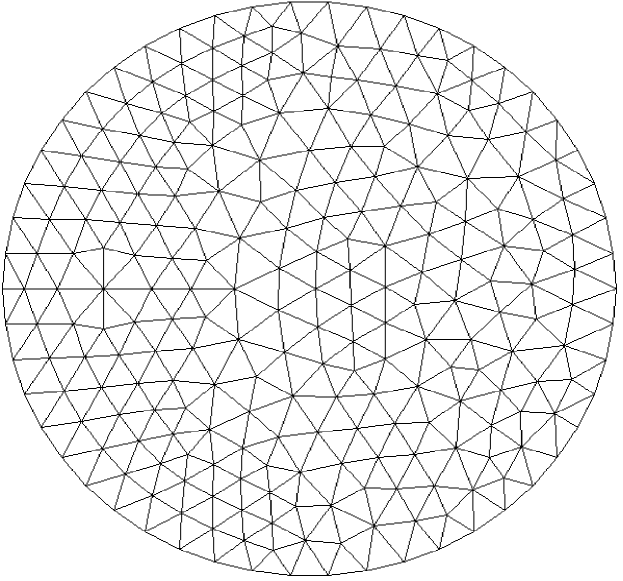
In two dimensions the element domains are typically triangles and quadrilaterals. In this work we use only triangles. In practice, mesh generation is carried out by using the software included in the general-purpose software package FEPG fpe . A typical mesh (domain discretization) for our example is given in Figure 3. Every element is equipped with a finite-dimensional functional space ${\cal F}_{\alpha}$, so that we approximate our physical solution locally, at every element, as a linear combination of functions of ${\cal F}_{\alpha}$ [usually, a special treatment of the boundary elements is required]. It is very common that the functional spaces ${\cal F}_{\alpha}$ are formed by piecewise polynomials. In this paper we consider linear elements, where the element functions are first-order polynomials, i.e. $a+bx+cy\,.$ This choice of element functions implies second-order convergence to the solution in the $L^{2}$ norm.

Figure 3: Mesh corresponding to the domain $\Omega$ in Equation (65).

A very important ingredient of the FEM is that it works with an integral form of the equation we want to solve, what is called the weak form of the problem. To obtain it, we multiply the equation (65) by a test function $\phi$, integrate over the domain $\Omega$, and use the Gauss or divergence theorem which introduces the boundary conditions (66). The result can be written in the form:

$${\cal L}[\phi,\psi]\equiv(\phi\,,\,\partial^{2}_{t}\psi)+(\nabla\phi\,,\,\nabla\psi)-2\int_{\partial\Omega}r\,\phi\,ds+2\,(\phi,1)=0\,,$$ (70)

where $(,)$ denotes the inner product $(u,v)\equiv\int_{\Omega}u\,v\,dxdy\,,$ $\nabla$ denotes the gradient operator, and $s$ is a coordinate on $\partial\Omega\,.$ It is important to note that the third term is the result of introducing into the weak formulation the boundary conditions (66).

Using the element functional spaces we can expand our solution in terms of nodal basis functions, $n_{A}(x,y)$ ($A=1,\ldots,N\,,$ being $N$ the number of nodes), which are associated with the nodes or grid points of the mesh. Nodal functions use to take the unity value at the node to which they are associated and zero at all the other nodes ($n_{A}(x_{B})=\delta_{AB}$ for any node $x_{B}$). Since we are going to produce a FEM discretization only in space, the expansion of our solution in terms of the nodal functions can be written in the form:

$$\psi_{h}\in H^{2}(\Omega)\,,~{}~{}~{}~{}\psi_{h}(t,x,y)=\sum_{B}\psi_{B}(t)\,n_{B}(x,y)\,,$$ (71)

where $H^{2}(\Omega)$ is the Sobolev space of functions on $\Omega$ that are, together with their first and second generalized spatial derivatives, square integrable, that is, they belong to $L^{2}(\Omega)\,.$ We are assuming that $\psi_{h}$ belongs to $H^{2}(\Omega)$ for any time $t\in[0\,,T]\,.$ The subscript $h$ denotes a scale associated with the domain discretization, for instance it may be proportional to the square root of the average area of the elements that compose the mesh. In our example $h$ refers to the maximum mesh diameter in the whole domain. An obvious property of $h$, is that the size of the elements goes to zero as $h$ goes to zero.

In a time-dependent problem like the one we are considering, the unknowns are going to be the functions $\psi_{A}(t)\,.$ The equations for these functions are obtained from the spatial discretization. In a Galerkin-type formulation of the FEM, the discretized equations come from the imposition of the vanishing of the residuals:

$${\cal E}_{A}={\cal L}[n_{A},\psi_{h}]=0\,,$$ (72)

which consists in taking $\phi=n_{A}$ in (70). Introducing also the expansion (71) yields the following system of equations for the functions $\psi_{A}(t)\,.$

$$\sum_{B}M_{AB}\ddot{\psi}_{B}+\sum_{B}K_{AB}\psi_{B}=F_{A}\,,$$ (73)

where the matrix $M_{AB}=(n_{A},n_{B})$, the so-called mass matrix, and the matrix $K_{AB}=(\nabla n_{A},\nabla n_{B})$, the so-called stiffness matrix, are symmetric and positive-definite matrices. The vector $F_{A}=-2(n_{A},1)+2\int_{\partial\Omega}rn_{A}ds$ is sometimes called the force vector. Equation (73) is the outcome of the FEM spatial discretization, which is sometimes called the semi-discrete form because it consist of a linear system of second-order ordinary differential equations in time. They are usually solved by using Finite-Differences methods. One of the most popular methods for second-order in time equations is the Newmark method, which is second-order accurate in time (see, e.g. Hughes (1987), for details).

Before we discuss the numerical implementation it is worth mentioning two important features of the FEM: (i) The piecewise approximations (piecewise linear in our example) of physical fields on finite elements provide good precision even with simple approximating functions. Increasing the number of elements we can achieve the desired precision. (ii) The local character of the approximation leads to sparse systems of equations once the problem is discretized. This helps considerably to solve problems with a very large number of nodal unknowns.

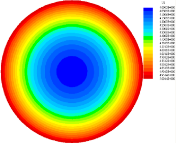
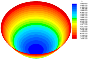
The numerical implementation of the equations of this paper has been carried out by using the general-purpose software package FEPG fpe , which can automatically generate finite element Fortran source code based on component programming. It can handle many types of problems, including time-dependent non-linear ones, like the one we are interested in. As a test, we have implemented the example described in this section in FEPG (see a snapshot of the evolution in Figure 4). We have also studied the convergence properties of the solution. Here, it is important to point out that in an unstructured mesh, like the one we are using in this example, to perform a convergence test is not as straightforward as it is for structured meshes. We have to define properly the scale $h$ such that by changing it we obtain the correct convergence. Starting from the initial mesh (see Figure 3), we call the solution we obtain $\psi_{h}$. Then, we globally refine this initial mesh by transforming every initial triangular element into four smaller triangular elements by connecting the three mid points of each edge. Solving our example equation on this mesh leads to a more accurate solution that we call $\psi_{h/2}$, and whose associated scale is $h/2$. By repeating this refinement process we get finer meshes, and by solving our equation on them we obtain more accurate solutions, $\psi_{h/2^{k}}$, with associated scale $h/2^{k}\,.$ We have checked that the solution we obtain converges quadratically in the scale $h$ to the exact solution (68) by studying the norms $\|\psi_{h/2^{k}}-\psi_{\mbox{\tiny exact}}\|_{L^{2}}$ (see the left of Figure 5). We have also checked that it convergences quadratically in the usual way, without making use of the exact solution, just by comparing the norms $\|\psi_{h}-\psi_{h/2}\|_{L^{2}}$ and $\|\psi_{h/2}-\psi_{h/4}\|_{L^{2}}$ (see the right of Figure 5).

Figure 4: Snapshots of the evolution of the solution of the example described by equations (65)-(67).

Figure 5: Convergence properties of the solution of the problem (65)-(67). On the left we show the convergence to the exact solution (68). On the right we show the $L^{2}$ convergence.

III.2 Finite Element Discretizations of the Toy Model

In this section, we are going to develop a FEM formulation for our toy model in the spirit of the ideas presented above. The ingredients of this problem are the following: (i) The computational domain was described in subsection II.4 and shown in Figure 1. (ii) The equations that describe our model are the PDEs given by equations (14,15). (iii) The boundary conditions and initial data are described in subsection II.4.

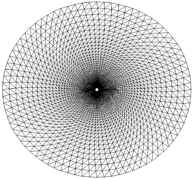
We start from the discretization of the computational domain (see Fig. 1). We use linear triangular elements. The aspect of the resulting triangularization is shown in Fig. 6. It is worth pointing out that the FEM is specially well suited for complex domains. In our case, this allows us to use circular boundaries, which adapt better to the characteristics of our problem. This is specially important in the case of the inner boundary, which corresponds to the fact that we have excised the black hole singularity from the computational domain.

Figure 6: Triangularization of the spatial domain given in Figure 1.

The next step in our development is the finite element discretization of the equations (14,15). We need to construct a weak formulation of these equations. To that end, it is very convenient to rewrite the equations in the following equivalent form:

$$\alpha^{-1}\partial_{t}\,\Phi = \alpha^{-1}\beta^{i}\,\partial_{i}\,\Phi\,+\Pi\,,$$ (74)

$$\alpha^{-2}\partial_{t}\,\Pi = \alpha^{-2}\beta^{i}\,\partial_{i}\,\Pi+\partial_{i}(\sqrt{h}\,h^{ij}\partial_{j}\Phi)+\alpha^{-1}a^{i}\,\partial_{i}\Phi+\alpha^{-1}K\Pi\ -4\,\pi\alpha^{-1}\,e^{\Phi}\,\rho\,,$$ (75)

where we have used the fact that $\alpha\sqrt{h}=1\,.$ The main reason for casting the equations in this form is that it brings the second-derivative terms into the form of the divergence of a spatial vector, without any additional factors. As we did with the example of the previous subsection, we are going to discretize the system of PDEs (74,75) for the unknowns $\Phi$ and $\Pi$ by using a FEM discretization (a Galerkin-type formulation) for the spatial dimensions and by using Finite Differences methods in time. In this sense, it is important to take into account that our system of equations is of first order with respect to time derivatives and of second order with respect to spatial derivatives. In order to discretize these equations, particular attention has to be paid to the convection terms in order to keep them under control. We deal with this issue by including additional artificial viscosity into the finite element equations that we obtain.

For the FEM spatial discretization the finite element space that we use is $S_{h}\subset H^{2}(\Omega)$, which consists of piecewise triangular linear interpolation functions. Then, taking all this into account and operating in a similar way as we did in the example of subsection III.1, the discretized problem that we obtain can be introduced in the following way: We need to find $(\Phi^{n+1}\,,\Pi^{n+1})\in S_{h}\subset H^{2}(\Omega)\,,$ such that the equations

$$(\alpha^{-1}\Phi^{n+1},\phi)=(\alpha^{-1}\Phi^{n},\phi)+(\Delta t\,\frac{\beta^{i}}{\alpha}\partial_{i}\Phi^{n},\phi)-\delta(h)(\Delta t\,\frac{\beta^{i}}{\alpha}\partial_{i}\Phi^{n},\Delta t\,\frac{\beta^{i}}{\alpha}\partial_{i}\phi\,)+(\Delta t\,\Pi^{n},\phi)\,,$$ (76)

$$(\alpha^{-2}\Pi^{n+1},\varphi) = (\alpha^{-2}\Pi^{n},\varphi)+(\Delta t\,\frac{\beta^{i}}{\alpha^{2}}\partial_{i}\Pi^{n},\varphi)-\delta(h)(\Delta t\,\frac{\beta^{i}}{\alpha^{2}}\partial_{i}\Pi^{n},\Delta t\,\frac{\beta^{i}}{\alpha^{2}}\partial_{i}\varphi)-\Delta t\,(\sqrt{h}\,h^{ij}\partial_{j}\Phi^{n+1},\partial_{i}\varphi){}$$ (77)

$$+ \Delta t\,(\frac{a^{i}}{\alpha}\partial_{i}\Phi^{n+1},\varphi)+\Delta t\,(\alpha^{-1}K\Pi^{n}\,\varphi)-\Delta t\,(4\pi\alpha^{-1}e^{\Phi^{n+1}}\,\rho,\varphi){}$$

$$- \int_{\partial\Omega_{out}}\frac{\alpha^{-1}}{(1+\frac{2M}{r})}(\Phi^{n+1}-\Phi^{n}+\frac{\Phi^{n+1}}{2r}\Delta t)\varphi\,ds-\Delta t\int_{\partial\Omega_{in}}\frac{\alpha^{-1}}{(1+\frac{2M}{r})}\frac{x^{i}}{r}\partial_{i}\Phi^{n+1}\varphi\,ds\,,$$

hold for any $(\phi,\varphi)\in S_{h}$ and for $n=0,1,\ldots,N\,,$ $N\Delta t=T\,,$ where $T=t_{f}-t_{o}$ is the total computational time. $\Delta t$ is the time-step size we use to evolve $\Phi$ and $\Pi\,.$ We use the notation $(\cdot,\cdot)$ to denote the inner product in $S_{h}$, which is defined as $(u,v)=\int_{\Omega}uvd\Omega~{}~{}~{}(\forall~{}u,v\in S_{h})$. Finally, to deal with the convection terms, arising from the derivatives of the fields along the shift vector, we use a streamline diffusion scheme that includes artificial viscosity and which is specially adapted to the FEM. The factor $\delta(h)$ is the penalty ratio of artificial viscosity, which of course depends on the mesh size $h$. It has to be tuned properly in order to obtain a stable computation and at the same time an accurate solution.

The last terms of (77) consist of integrals on the boundaries $\partial\Omega_{in}$ and $\partial\Omega_{out}$. The way they come into play is the following: In the case of the outer boundary $\partial\Omega_{out}$, we obtain the last but one integral in (77) after integration by parts of the term with second-order spatial derivatives in (75) and imposition of the outgoing boundary condition (42). In the case of the inner boundary $\partial\Omega_{inn}$, we obtain the last integral in (77) from the same integration by parts. However, the resulting integral does not correspond to a proper boundary condition. As we have already mentioned before, we do not need any boundary condition at the inner boundary due the particular structure of the characteristics there (remember that the inner boundary is inside the horizon), which all point inwards. Therefore, the resulting integral is just an integration of a term proportional to $\partial_{i}\Phi^{n+1}$ on the inner boundary.

Equations (76,77) are the basis of the computational procedure that we follow to obtain the solution of our problem. The basic algorithm consists in computing first $\Phi_{n+1}$ from (76) in terms of $\Phi_{n}$ and $\Pi_{n}$. The next step is to introduce $\Phi_{n+1}$ into the right-hand side of (77) to obtain $\Pi_{n+1}$ in terms of $\Phi_{n}$ and $\Pi_{n}$ together. Then, $\Pi_{n+1}$ has to be used in order to compute the value of $\Phi$ in the next time step, and so on. It is not difficult to show that this algorithm is second-order accurate both in space and in time.

III.3 Computing the Motion of the Particle

In the procedure we have just described we have omitted the role of the motion of the particle. It is clear that in order to evaluate the right-hand side of (77) we need to introduce the position of the particle. And for that, we need to solve the set of equations (22,23). These ODEs have to be integrated simultaneously with the PDEs, which means that every time we evaluate the right-hand of (77) we need to evolve them a time step $\Delta t\,.$ And then, to use use the outcome of the integration of the ODEs (new position and velocity of the particle) in order to evaluate the source of equation (15) [equation (77) in the discretized system].

The type of numerical algorithm we use to solve the ODEs (22,23) has to take into account the particular structure of the equations (23), which are the non-trivial ones. These equations contain two differentiated terms, $f^{i}_{\mbox{\footnotesize g}}$ and $f^{i}_{\Phi}$. The first term would give us the geodesic motion around a Schwarzschild Black Hole, and therefore the time scale of the changes induced by the term $f^{i}_{\mbox{\footnotesize g}}$ is the orbital period of the geodesic that the particle would follow by ignoring the radiation reaction effects. The second term contains the gradients of the scalar field $\Phi$ in the neighbourhood of the particle position. These terms are the responsible, in our toy model, of the radiation reaction effects, and therefore, the time scale of the changes they induce will be in general much smaller than the orbital time scale.

Taking into account that these ODEs are nonlinear both in $z^{i}$ and in $v^{i}$, we are just going to use an explicit scheme with a time step $\Delta t_{s}$ much smaller than the PDE time step $\Delta t\,.$ That is, we split each PDE time step $\Delta t$ in many ODE time steps $\Delta t_{s}\,,$ so that we solve equations (22,23) in each time step $\Delta t_{s}$ in order to guarantee the accuracy of the solution. This scheme is able to approximate the accuracy that an implicit scheme would have provided. The specific discretization algorithm we use in our numerical computations to evolve the particle’s position, ${\bm{z}}$, and velocity, ${\bm{v}}$, from a PDE time step $t_{n}$, with values $({\bm{z}}^{n},{\bm{v}}^{n})\,,$ to the next time step $t_{n+1}$, with values $({\bm{z}}^{n+1},{\bm{v}}^{n+1})$ is given by:

$$\begin{array}[]{l}{\bm{v}}_{0}^{n+1}={\bm{v}}^{n}\,,\\ {\bm{z}}_{0}^{n+1}={\bm{z}}^{n}\,,\\ \mbox{\tt From $m=0$ to $m=M-1\,$:}\\ ~{}~{}~{}~{}{\bm{v}}_{m+1}^{n+1}={\bm{v}}^{n}+\Delta t_{s}\,\left\{{\bm{f}_{\mbox{\footnotesize g}}}\left[{\bm{v}}_{m}^{n+1},{\bm{z}}_{m}^{n+1}\right]+{\bm{f}_{\Phi}}\left[{\bm{v}}_{m}^{n+1},{\bm{z}}_{m}^{n+1},\Pi^{n},\nabla\Phi^{n}\right]\right\}\,,\\ ~{}~{}~{}~{}{\bm{z}}_{m+1}^{n+1}={\bm{z}}^{n}+\Delta t_{s}\,{\bm{v}}_{m+1}^{n+1}\,,\\ {\bm{v}}^{n+1}={\bm{v}}_{M}^{n+1}\,,\\ {\bm{z}}^{n+1}={\bm{z}}_{M}^{n+1}\,,\end{array}$$ (78)

where $\Delta t_{s}$ denotes the ODE time step, which is related to the PDE time step by the relation $\Delta t_{s}=\Delta t/M\,.$ We choose the integer $M$ in order to achieve the accuracy we want. The way in which $\nabla\Phi$ is computed is by using the corresponding FEM piecewise polynomial expansion that follows from the expansion in nodal functions of $\Phi\,.$

III.4 The Adaptive Finite Element Method

The AFEM is the application of the classical FEM on a series of local adaptive meshes in order to get more accurate numerical results with less computational cost. Starting with a given initial coarse mesh, the adaptive mesh on each level is generated locally and adaptively in terms of a posteriori error estimate of the finite element solution. Usually local refinement takes place in places where the a posteriori errors are much bigger than elsewhere, or in other words, where the finite element solution changes steeply. On the other hand, for those places in which the a posteriori errors are sufficiently small, the local derefinement will operate in order to eliminate extra grids because in those places the solution changes slowly. Thus, during the finite element computation we can adaptively adjust the mesh density without losing the numerical accuracy but reducing considerably the computational cost.

It is obvious that the key part of the AFEM is the a posteriori error estimate. To have a good such estimate means that one can precisely find out in which places the mesh should be refined or derefined without introducing much numerical pollution. After this is done, the rest of the procedure is standard. For instance, the mesh bisection and the finite element approximation. There is presently a number of works in the literature on these issues (see, e.g. Morin et al. (2002); Rivara and Venere (1996); Rivara and Iribarren (1996); Dolejsi (1998)). In what follows we introduce our own a posteriori error estimate, which is an interpolation error estimate. Then, we elaborate on our local mesh improvement techniques such as refinement, coarsening, and the smoothing strategy, which aim to minimize the interpolation error.

The interpolation error estimate comes from recent work by Chen, Sun, and Xu Chen et al. (2003). This estimate can be seen as the theoretical foundations of our adaptive mesh techniques, that is, our algorithms are aimed at minimizing (or at least reducing) the interpolation error by iteratively modifying the grids. We introduce the estimate through the following definition: “Let $\Omega$ be a bounded domain in $\mathbb{R}^{n}\,.$ Given a function $u\in\mathcal{C}^{2}(\bar{\Omega})$, we say that a symmetric positive definite matrix $H\in\mathbb{R}^{n\times n}$ is a majoring Hessian of $u$ if

$$|\xi^{t}(\nabla^{2}u)(\mathbf{x})\xi|\leq c_{0}\xi^{t}H(\mathbf{x})\xi\,,\quad(\xi\in\mathbb{R}^{n}\,,~{}\mathbf{x}\in\Omega)\,,$$ (79)

for some positive constant $c_{0}$”. Here, $\xi^{t}$ denotes the transpose of the vector $\xi\,.$ We then use the majoring Hessian to define a new metric

$$H_{p}=(\det H)^{-\frac{1}{2p+n}}H\,,\quad(p\geq 1)\,.$$ (80)

There are two conditions for a triangulation $\mathcal{T}_{N}$, where $N$ is the number of simplexes (generic elements), to be a nearly optimal mesh in the sense of minimizing the interpolation error in the $L^{p}$ norm. The first condition consists in asking the mesh to capture the high oscillations of the Hessian metric, that is, $H$ should not change very much on each element. This condition can be expressed in a more precise way by means of the following statement: “There exists two positive constants $\alpha_{0}$ and $\alpha_{1}$ such that

$$\alpha_{0}\xi^{t}H_{\tau}\xi\,\leq\,\xi^{t}H(\mathbf{x})\xi\,\leq\,\alpha_{1}\xi^{t}H_{\tau}\xi\,,\quad(\xi\in\mathbb{R}^{n}\,,~{}\mathbf{x}\in\Omega)\,,$$ (81)

where $H_{\tau}$ denotes the average of $H$ over $\tau\in\mathcal{T}_{N}$”. The second condition demands the triangularization $\mathcal{T}_{N}$ to be quasi-uniform under the new metric induced by $H_{p}$. This condition can also be express in a more precise way through the following statement: “There exists two positive constants, $\beta_{0}$ and $\beta_{1}$, such that

$$\frac{\sum_{J}\tilde{d}_{\tau,J}^{2}}{\left|\tilde{\tau}\right|^{\frac{2}{n}}}\,\leq\,\beta_{0}\quad(\forall\tau\in\mathcal{T}_{N})\quad{\rm and}\quad\frac{\max_{\tau\in\mathcal{T}}\left|\tilde{\tau}\right|}{\min_{\tau\in\mathcal{T}}\left|\tilde{\tau}\right|}\,\leq\,\beta_{1}\,,$$ (82)

where $|\tilde{\tau}|$ denotes the volume of $\tau\,,$ and $\tilde{d}_{\tau,J}$ the length of the $J$-th edge of $\tau$ under the new metric $H_{p}\,.$ The first inequality in (82) means that each $\tau$ is shape-regular under the metric $H_{p}$. The second inequality means that all elements $\tau$ are of comparable size (also under the new metric), which is a global condition. This means that the mesh is more dense at the regions where $\det H_{p}(\mathbf{x})$ is larger. In Chen et al. (2003), it has been proven the important result that a triangulation that satisfies both the local condition (81) and the global one (82) yields a good approximation. This result can be expressed in a precise way in the form of a theorem: “Let $u$ be a function belonging to $\mathcal{C}^{2}(\bar{\Omega})$, $\mathcal{T}_{N}$ a triangularization satisfying the conditions (81) and (82), and $u_{\cal I}$ the linear finite element interpolation of $u$ based on the triangulation $\mathcal{T}_{N}\,.$ Then, the following error estimate holds:

$$\left\|u-u_{\cal I}\right\|_{L^{p}(\Omega)}\;\leq\;CN^{-\frac{2}{n}}\left\|\sqrt[n]{\det(H)}\right\|_{L^{\frac{pn}{2p+n}}(\Omega)}\,,$$ (83)

for some constant $C=C(n,p,c_{0},\alpha_{0},\alpha_{1},\beta_{0},\beta_{1})$. This error estimate is optimal in the sense that for a strictly convex (or concave) function, the above inequality holds in a reversed direction.”

The result expressed by this theorem is the basis of the grid adaptation algorithms that we use in this work. Roughly speaking, for a given function $u$, we will adapt our grids in such a way that the conditions given in (81) and (82) are satisfied in the best possible way. One important remark we need to make is that the validity of the theorem stated above allows for a few exceptions of the condition (82) for $p<\infty$ (see Chen et al. (2003) for details). This is of particular importance since in practice it is very difficult to guarantee that the condition (82) is satisfied everywhere.

The next point is to see how the Hessian matrix of the solution can be obtained when the linear finite element approximation is used for the discretization of the PDEs of our problem. Since taking piecewise second derivatives of piecewise linear functions will give no approximation to the Hessian matrix, special post-processing techniques need to be used in order to obtain a reasonable Hessian matrix approximation from linear finite elements. One of the most popular techniques is the patch recovery technique proposed by Zienkiewicz and Zhu (ZZ) Zienkiewicz and Zhu (1992a, b), which is based on the least squares fitting on local patches. Results from the application of this technique demonstrate that it is robust and efficient. The theoretical reason why the ZZ method works is largely understood to be related to the superconvergence phenomenon for second-order elliptic boundary-value problems discretized on a finite element grid that has certain local symmetry (see the works of Walhbin Wahlbin (1995) and Babuška and Strouboulis Babuška and Strouboulis (2001)). These classic superconvergence results can be used in order to justify the effectiveness of the ZZ method. A significant improvement of this type of analysis was introduced recently by Bank and Xu Bank and Xu (To appeara, To appearb). In Bank and Xu (To appeara) they give superconvergence estimates for piecewise linear finite element approximations on quasi-uniform triangular meshes where most pairs of triangles that share a common edge form approximate parallelograms. In Bank and Xu (To appeara) they also analyze a post-processing gradient recovery scheme, showing that $Q_{h}\nabla u_{h}$, where $Q_{h}$ is the global $L^{2}$ projection, is a superconvergent approximation to $\nabla u$. This result leads to a theoretical justification of the ZZ method for such type of grids (see Xu and Zhang Xu and Zhang (Article electronically published on August 19, 2003) for details).

The gradient recovery algorithm that we use in the numerical examples of this paper is based on a new approach due to Bank and Xu Bank and Xu (To appearb), where they use the smoothing iteration of the multigrid method to develop a post-processing gradient recovery scheme. This scheme proves to be very efficient for recovering Hessian matrices. All the methods mentioned above can be extended to anisotropic grids with some appropriate modifications, but a theoretical justification of such extensions is still lacking. Nevertheless, numerical experiments have given satisfactory results.

Let us now discuss techniques to improve the mesh quality. We define the mesh quality of a given triangulation $\mathcal{T}$ in terms of the interpolation error:

$$Q(\mathcal{T},u,p)=\left\|u-u_{{\cal I},\mathcal{T}}\right\|_{L^{p}(\Omega)}\,,\quad(1\,\leq\,p\,\leq\,\infty)\,.$$ (84)

There are three main ways of improving a mesh: (i) Refinement or coarsening through splitting or merging of edges Bank et al. (1983); Rivara (1984); Kornhuber and Roitzsch (1990); (ii) edge swapping by replacing sets of elements by other such sets while preserving the position of the points (nodes) Lawson (1977); and (iii) mesh smoothing, which moves the vertexes of the mesh while keeping the connectivity Field (1988); Bank and Smith (1997); Shephard and Georges (1991); Freitag et al. (1995). We derive those techniques by minimizing the interpolation error in the $L^{p}$ norm.

For the first method, this can be done by equidistributing the edge lengths with respect to the new metric. Thus, we compute the edge lengths with respect to the new metric $H_{p}$ and mark edges whose length is greater than $r_{1}\,d$, where $r_{1}\geq 1$ is a parameter and $d$ is a fixed edge length, the global average edge length. Then, we connect marked edges element-wise according to the different situations that can be given. This is illustrated in Figure 7. The coarsening operates like an inverse procedure to the refinement process. It marks the edges whose length is smaller than $r_{2}\,d$, where $r_{2}\leq 1$ is another parameter. We then shrink this edge to a point and connect to the vertexes of the patch of the edge.

Figure 7: Edge based refinement.

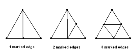
We consider now the case of edge swapping involving four points $\{\mathbf{x}_{\alpha}\}$ ($\alpha=1-4$) constituting two adjacent triangles and a convex quadrilateral. Let $\mathcal{T}_{1}=\triangle_{123}\cup\triangle_{134}$ and $\mathcal{T}_{2}=\triangle_{124}\cup\triangle_{234}$ be two triangularizations, where $\triangle_{\alpha\beta\gamma}$ stands for the triangle made up of the points $\mathbf{x}_{\alpha}\,,$ $\mathbf{x}_{\beta}\,,$ and $\mathbf{x}_{\gamma}\,.$ Then, we choose the triangulation $\mathcal{T}_{1}$ if and only if $Q(\mathcal{T}_{1},u,p)\leq Q(\mathcal{T}_{2},u,p)\,,$ for some $1\leq p\leq\infty\,.$ In Chen and Xu (2004), we show this criteria is equivalent to the empty circle criteria when $u(\mathbf{x})=\|\mathbf{x}\|^{2}\,.$ Thus it is an appropriate generation of the edge swapping used in the isotropic case to the anisotropic case.

Finally, local smoothing of the mesh adjusts the location of a vertex in its patch $\Omega_{\alpha}$, which consists of all simplexes containing the vertex $\mathbf{x}_{\alpha}$, without changing the connectivity. The moving of a vertex to its new location is expected to improve the quality of the mesh. Several sweeps throughout the whole mesh can be performed to improve the overall mesh quality. By minimizing the interpolation error in $\Omega_{\alpha}$, we move the vertex $\mathbf{x}_{\alpha}$ to the position $\mathbf{x}^{*}$ in such a way that

$$\nabla u(\mathbf{x}^{\ast})=-\frac{1}{\left|\Omega_{\alpha}\right|}\sum_{\tau_{\beta}\in\Omega_{\alpha}}\Big{(}\nabla\left|\tau_{\beta}\right|\sum_{\begin{subarray}{c}\mathbf{x_{\gamma}}\in\tau_{\beta}\\ \mathbf{x_{\gamma}}\neq\mathbf{x_{\alpha}}\end{subarray}}u(\mathbf{x_{\gamma}})\Big{)}\,.$$ (85)

The derivation of this formula can be found in Chen and Xu (2004).

For the application to our numerical computations we use $Q_{h}\nabla u_{h}$ and $u_{h}$ in (85). Moreover, we need to make choices for the different parameters of this adaptive mesh technique. For the order of the $p$ of the $L^{p}$ norm we use $p=1$, the $L^{1}$ norm. According to Chen and Xu (2004), the $L^{1}$ norm can catch singularities more efficiently than other norms. For the multiple $r$ ($r_{1},r_{2}$ in the text) of the global average edge length $d$ under the new metric $H_{p}$ (we use $rd$ as the threshold to determine which edge lengths under the new metric are bigger than it, we will then bisect those edges in the local refinement process) we take $r=3$ initially. Our local refinement procedure is a nested iteration process. There is an outer iteration for which, on each step, we reduce the multiple $r$ till $r_{min}$ (we take $r_{min}=1$). The main purpose of this iteration is to resolve the singularity as precisely as possible and to control the refinement pollution at the lowest level. On each outer iteration step, we perform an inner iteration, and there another number $r$ to control this iteration. Usually we do not need this number to establish a criterion to stop the inner iteration of local refinement. For the sake of getting the optimal mesh, we let this iteration go until all the edge lengths are smaller than $rd$ as before. In practice there are occasions when this may take too much time, and in those cases we set up a criterion as the ones before in order to control the number of inner iterations.

IV Numerical Results

In this section we report the results of the simulations of the toy model. We have distinguished two types of simulations. Those that were performed by just using the classical FEM, without adding any extra adaptivity. The results are discussed in subsection IV.1. And those that were performed by using the AFEM described in the previous section. The results of these simulations are discussed in subsection IV.2.

IV.1 Numerical simulations of the toy model using the FEM

The mass ratio we have considered is $\mu=0.01$, that is the particle’s mass is $m=0.01\,M\,.$ The inner boundary is located at $r_{in}=1\,M$, inside the horizon $r_{h}=2\,M\,.$ The outer boundary has been located at $r_{out}=50\,M$. Regarding the initial data, the only parameters that need to be given, in addition to the ones already given, in order to completely specify it [see subsection II.4] are the width of the Gaussian that we use to regularize the Dirac delta distribution, which we take to be $\sigma=1\,M$, and the initial position of the particle, which we take to be $(x_{o},y_{o})=(10\,M,0)\,.$ Finally, we give the resolution that we have used for the simulations. To give a measure of the spatial resolution we describe the structure of the mesh. It is composed of $N=9266$ triangles, quasi-uniformly distributed, more concentrated near the center and coarsening gradually as we approach the outer boundary. Regarding the resolution in the time direction, the step size we use for the time evolution is $\Delta t\,=0.01\,M$. The algorithm we use to study the evolution of the gravitational scalar field $\Phi$ and the motion of the particle is completely described by the explicit schemes of equations (76,77) and (78).

What we have observed is that the orbit of the particle (remember that the initial data corresponds to a circular orbit in the absence of the scalar gravitational field) shrinks gradually until the particle reaches the horizon at $r_{h}=2\,M$. The trajectory followed by the particle is drawn in Figure 8. Snapshots characterized by the time $t$ and time-step number $n$ of the evolution of the scalar gravitational field are shown by means of the contour plots given in Figures 9-13. The position of the particle is evident in these graphs.

We have checked the energy-balance law (64) for the parameters given above. The result can be found in Figure 14, where the horizontal axis denotes the time and the vertical axis indicates the value of the left-hand side of (64) in units of $m\,$. As we can see there, the energy law (64) is satisfied up to a certain level along the evolution. However, from $t=40\,M$ the error in the energy-balance test grows and stabilizes around a different but bigger value. This growth is due to outer boundary effects: The particle started from a position $r=10\,M$ and the outer boundary is located at $r=50\,M\,.$ As we have mentioned in the discussion of the boundary conditions in subsection II.4, the outer boundary condition (42) is not optimal, and induces some error in the solution. This could be improved by either moving the outer boundary further out or by using an improved outer boundary condition.

Figure 8: Trajectory followed by the particle.

Figure 9: Scalar gravitational field $\Phi$ at time $t=10\,M$ (n=1000) [left] and at time $t=20\,M$ (n=2000) [right].

Figure 10: Scalar gravitational field $\Phi$ at time $t=30\,M$ (n=3000) [left] and at time $t=40\,M$ (n=4000) [right].

Figure 11: Scalar gravitational field $\Phi$ at time $t=50\,M$ (n=5000) [left] and at time $t=100\,M$ (n=10000) [right].

Figure 12: Scalar gravitational field $\Phi$ at time $t=200\,M$ (n=20000) [left] and at time $t=300\,M$ (n=30000) [right].

Figure 13: Scalar gravitational field $\Phi$ at time $t=400\,M$ (n=40000) [left] and at time $t=500\,M$ (n=50000) [right].

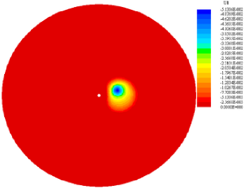
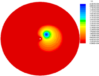
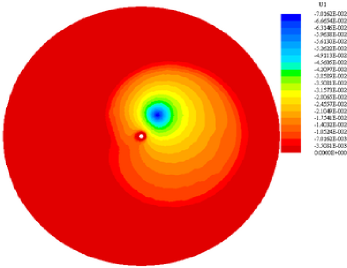
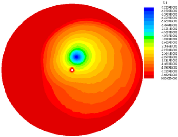
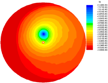
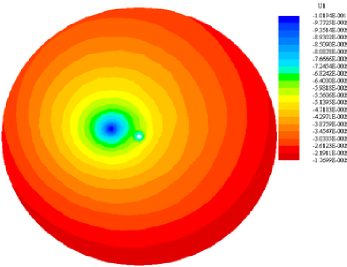
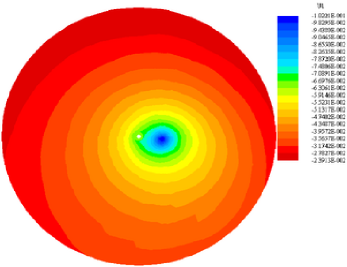
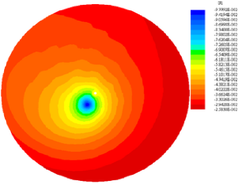
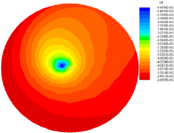
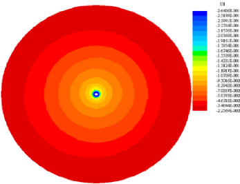
The key point in these computations is the ability of our numerical scheme to resolve the source term describing the particle. It enters the equations for the scalar gravitational field $\Phi$ as a very singular source term. This source term depends on the position of the particle, but at the same time, the position of the particle depends of the gradients of $\Phi\,.$ Therefore, it is very important first to compute properly the effect of the source $\rho$ on the field $\Phi$, and then to compute accurately the gradient of the field itself. We have already mentioned that in the computations shown in this subsection the width of the Gaussian has been taken to be $\sigma=1\,M$ in order to make the source sufficiently smooth for the resolution we have used. In this sense, if we try to use a smaller width, for instance $\sigma=0.1\,M\,,$ the classical FEM will fail to provide the expected accuracy, although it still provides a numerical solution. Here is where one realizes the potential of the AFEM as a better choice to carry numerical computation for a model presenting features similar to the ones of our model. In the next subsection we describe how we have implemented the AFEM in the case of the toy model and show that it provides a reasonable solution for the case in which $\sigma=0.1\,M\,.$

Figure 14: Energy-Balance Test for the simulation with the FEM (no additional adaptivity).

IV.2 Numerical simulations of the toy model using the AFEM

We have just concluded that the central part of the numerical simulation of our toy model, and more in general of EMRBs, is the proper resolution of the matter source, $\rho\,,$ and of the gravitational field, $\Phi\,,$ in the surroundings of the particle position, which is a key issue in order to compute accurately the motion of the particle and hence, the waves that are emitted as a consequence. To that end, within the framework we have established above, we want to able to compute accurately for small values of the particle’s width $\sigma$. In the limit $\sigma\rightarrow 0$ we recover the distributional description of the particle’s that appears in the continuum description. Then, it is obvious that better accuracy in the terms discussed above means to increase the resolution around the particle’s position, and in this sense the AFEM is a natural choice since it provides the resolution required at the different regions of the computational domain, which maintains the computational cost at realistic levels.

According to the theoretical foundations of the adaptive mesh technique presented above, in order to apply mesh adaptivity successfully in our numerical computations, first of all, we have to study which quantity in the problem we are dealing with can be used in order to determine where and how the mesh should be refined. In technical terms this means that we have to be able to determine the places where refinement (or derefinement) has to take place in terms of the Hessian matrix of the selected quantity. We have to look for place where the majoring Hessian matrix is much bigger than anywhere else, which are the places where the quantity we have chosen changes very fast. In the case of our toy model there is no too much choice. We can either take the field $\Phi$ or the source $\rho$. In the case of $\Phi$, it is interesting in the sense that it is one of the goals of our computations. However, since it is the solution of a wave-type equation, it evolves like a wave in the sense that the profile of the solution will have maxima and minima which will be captured by the adaptive mesh procedure, and hence most parts of the domain will be eventually refined, and this may not be the most efficient way to proceed. The other choice, the particle’s source $\rho\,,$ is a better choice for the simple reason that we are also solving for the particle’s position at the same time that we are solving the PDEs for the field. Therefore, the recognition of the regions that need refinement is going to be simpler in our problem. That is, the most efficient way of adapting the mesh for our computations is to concentrate on the region where the particle is present and follow it from there.

If we look at the behaviour found in the previous subsections (see Figures 9-10), it happens that the bigger values of $\Phi$ occur around the particle’s position. Therefore, refining there is very convenient at that stage of the computation. A possible drawback of using the particle’s source as the refinement criterion is that the situation changes at later times when the field $\Phi$ is present all over the computational domain and it may be a need for refinement in other places like close to the horizon. However, in the numerical simulations we have performed we find that using the source term $\rho$ for refinement is much better than using the field $\Phi\,.$ By calculating the Hessian matrix of the particle’s source we can exactly know where and how to get local mesh refinement on the particle.

For the numerical simulations of the toy model with the AFEM we use the same parameters as in subsection IV.1, excepting for the width of the Gaussian, which we have been able to reduce down to $\sigma=0.1\,M\,.$ And this has been done using a number of triangular elements in the interval $11000-15000$ (the number of elements changes with the evolution, depending on how the adaptivity is implemented), a number comparable to the one used in the calculations without adaptivity. That is, working with the AFEM we have been able to use a width $\sigma$ an order of magnitude smaller than with the classical FEM, using a comparable number of elements. The time step is now $\Delta t=0.005M\,,$ half the one used in the previous simulations. The trajectory followed by the particle is drawn in Figure 15. We show the evolution of the scalar gravitational field in Figures 16-20. These are contour plots as the ones we used previously. In order to show how we refine the mesh in the evolution we have superposed the mesh to the contour plots. In this way we can see how the high-resolution part of the mesh moves with the particle. One can clearly see the difference between this case and the previous case: the particle inspirals much faster in this case, and it hardly completes more than one orbit. To understand this difference, it is important to remark the fact that the particle sources are different since the Gaussian profiles have a different width $\sigma$ and the fact that the sources couple non-linearly with the scalar gravitational field. As a consequence, the difference in $\sigma$ leads to a different evolution. We have checked that when take $\sigma=1M$ with the AFEM we recover the type of trajectories we get in the case without adaptivity.

Figure 15: Trajectory followed by the particle.

Figure 16: Scalar gravitational field $\Phi$ at time $t=5\,M$ (n=1000) [left] and at time $t=20\,M$ (n=4000) [right].

Figure 17: Scalar gravitational field $\Phi$ at time $t=35\,M$ (n=7000) [left] and at time $t=50\,M$ (n=10000) [right].

Figure 18: Scalar gravitational field $\Phi$ at time $t=65\,M$ (n=13000) [left] and at time $t=80\,M$ (n=16000) [right].

Figure 19: Scalar gravitational field $\Phi$ at time $t=95\,M$ (n=19000) [left] and at time $t=110\,M$ (n=22000) [right].

Figure 20: Scalar gravitational field $\Phi$ at time $t=125\,M$ (n=25000) [left] and at time $t=140\,M$ (n=30000) [right].

Figure 21: Scalar gravitational field $\Phi$ at time $t=150\,M$ (n=25000) [left] and at time $t=160\,M$ (n=32000) [right].

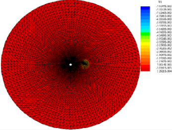
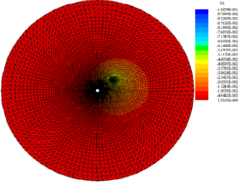
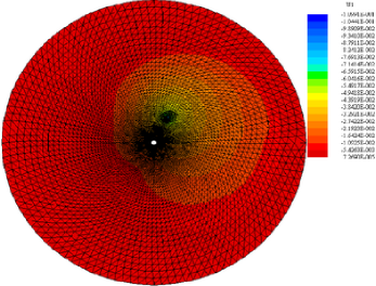
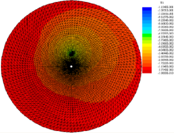
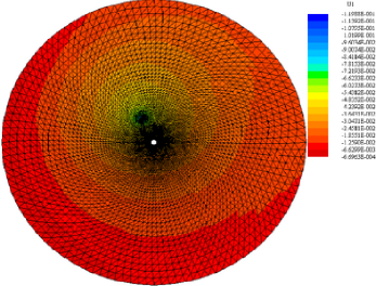
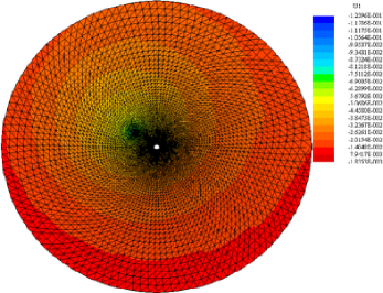
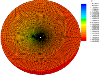
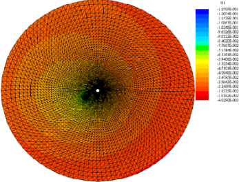
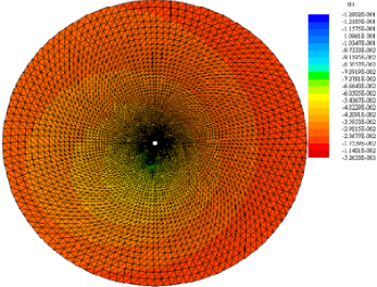
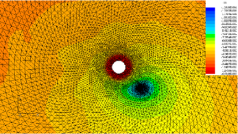
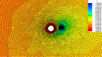
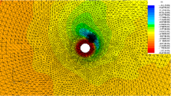
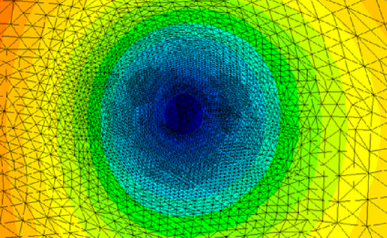
A more detailed view of the structure of the refined region around the particle is shown in Figure 22, where one can see the different levels of refinement, and how the resolution increases as one approaches the particle. A global perspective of the structure of the mesh, containing the excised region around the singularity of the black-hole, and the refined region around the particle can be seen in the three-dimensional graph shown in Figure 23.

Figure 22: Details of the refinement used around the particle’s position.

Figure 23: A three-dimensional visualization of the mesh including the excised region and the refinement around the particle.

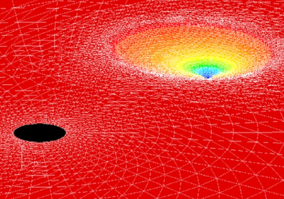
We have also checked the energy-balance law (64) for the simulations with adaptivity. We have plotted the result in Figure 24, where again the horizontal axis denotes time and the vertical axis the value of the left-hand side of (64) normalized with the mass $m$ of the particle. The behaviour of the error in the conservation law is very similar to the one in the case without adaptivity, where the error in the energy-balance test grows after the boundary affects the particle. In this case, the error does not seem to stabilize as clearly as in the previous case, and in average the error in the conservation law is bigger. However, one has to take into account that the evolution in this case is much faster since the particle has plunged very quickly. Moreover, since the number of elements in both cases is comparable, but in the case of the AFEM a considerable amount of them have been used to increase the resolution around the particle, this means that the density of elements near the boundaries is less and therefore if errors are propagated from there, they can affect more the result than in the case without adaptivity. This can be avoided by using more computational power to push the boundaries far enough so that we can neglect their effect during the significant part of the evolution.

Figure 24: Energy-Balance Test for the simulation that uses the AFEM.

V Remarks and Conclusions

In this work we have studied the application of Finite Element techniques to the time-domain numerical simulations of EMRBs. More specifically, we have shown how Finite Elements can help us in achieving the degree of adaptivity that the computation of radiation reaction effects around the small body requires. However, adaptivity is not the only advantage in using Finite Elements for the study of EMRBs, some of which are obvious from the study of the toy model we have considered in this work. In short, the main additional advantages that Finite Elements provide are: (i) Versatility. the FEM can be applied to a wide range of problems: static, quasi-static, transient, highly dynamical, linear and nonlinear, etc. Moreover, the practical implementation of the FEM can be easily designed in a modular way, as it shown by the existence of a number of multi-purpose Finite Element packages. This is a good property for the design of complex numerical codes, as the ones one may need for the description of astrophysical EMRBs. (ii) Many of the procedures that one uses in the framework of the FEM have a solid theoretical foundation, in the sense that behind them one often finds rigorous mathematical analysis (examples of this can be found in the classical textbooks Strang and Fix (1973); Zienkiewicz (1977); Ciarlet (1978); Hughes (1987); Babuška and Strouboulis (2001)). (iii) The ability of the FEM to manage problems with complex geometries. For instance we can easily consider spherical boundaries which is helpful in imposing boundary conditions and also in implementing excision techniques for black hole singularities. This is something that may be worth to export to fully numerical relativistic calculations of spacetimes containing black holes. (iv) In relation with the previous issue, the imposition of boundary conditions can be done in a somewhat natural way in a FEM framework. The idea is that by adapting the mesh to the geometry of the problem under study, boundary conditions which are also adapted to that geometry will be incorporated in a natural way into the FEM discretization through the weak formulation of the problem. The outgoing boundary conditions that we have used in our toy model are a good example, its implementation is simpler that it would have been in a similar Finite Differences scheme. (v) Another advantage of the FEM, that we have not explored in this paper, is that it is to some extent natural to handle distributions, like for instance the typical Dirac delta distributions that appear in physical systems containing particles (e.g., EMRBs). The idea is that we can use the exact properties of the distributions at the level of the weak formulation of the equations, which in the case of Dirac delta distributions leads automatically to a regularization of the singularity associated with that kind of distributions. We can apply this idea, for instance, to the calculation of the general-relativistic perturbations of a non-rotating black hole, produced by the presence of a point-like object, via the Regge-Wheeler-Zerilli formalism. Then, the type of FEM discretization we would get is similar to the one obtained by Price and Lousto Lousto and Price (1997); Martel and Poisson (2002); Martel (2004), where they also used an integral form of the equations in order to obtain a discretization. In addition, the FEM procedure can be generalized to higher-dimensional problems in a straightforward way. These ideas will be the subject of future investigations

In this paper we have illustrated the capabilities of the FEM and its suitability to simulate EMRBs, by applying it to a simplified model, a toy model that retains the basic ingredients and difficulties of general relativistic EMRBs. We have shown simulations of this system based on the classical FEM and simulations based on the AFEM. An outcome of this work is the realization that in order to increase the resolution around the small body, treated as a particle, the introduction of adaptivity in the region of the particle is necessary and in this sense the AFEM is a natural tool to use. The primary benefit of the AFEM is that it can provide an efficient, accurate and reliable computational analysis of very large continuum problems, for only a relatively small fraction of the cost associated with the non-adaptive FEM. The accuracy of a finite element solution is directly dependent on the number of free parameters used to mathematically represent the problem, and how effectively those parameters, or mathematical degrees of freedom, are distributed over the problem space. Furthermore, the full computational cost associated with obtaining a finite element solution is related to both the number and the interconnectivity of the degrees of freedom used in the problem discretization. Consequently, the most efficient distribution of degrees of freedom for a problem is the one that provides a sufficiently accurate solution for the lowest number of free parameters. Currently, the only practical way to achieve this objective is by using adaptive solution strategies which are capable of cleverly evolving and improving an efficient distribution of degrees of freedom over the problem domain by establishing solution error distributions, and then adjusting or adding degrees of freedom to the discretization in order to correct them. By increasing the numbers of degrees of freedom only in the regions of higher error in the solution, it is possible to make the most significant improvement in the global accuracy of the finite element solution for the minimum additional computational cost. In this paper we employed the Hessian matrix of the solution to describe the solution error distribution, which can perfectly guide us to where and how we have to locally refine the mesh without any unnecessary pollution. In this sense, it is important to emphasize that the rest of adaptive strategies available do not have this advantageous property. Moreover, this comes without paying an extra price since the main advantages of the other adaptivity techniques are present in the AFEM that we have used.

The natural continuation of this work is the transfer of the technology used here to the general relativistic problem. One possible way is to consider the general framework of metric perturbations in the setup of the 3+1 decomposition, that is, to use 3D perturbative numerical relativity, trying at the same time to profit from the experience gained in 3D full numerical relativity. However, 3D calculations using the AFEM may be at present computationally too demanding and therefore, other avenues should be also explored. Among them we can consider 1D calculations restricted to the case of a non-rotating MBH, by using the well-known Regge-Wheeler and Zerilli-Moncrief formalisms, or just by using a harmonic gauge, where the computation of self-forces seems more natural. This would be an interesting benchmark to test further the FEM techniques in a general-relativistic context. From here, one can study problems of more interest for gravitational wave physics related to LISA (involving spinning MBHs) by considering 2D calculations using the curvature based formalism of Teukolsky for linear perturbations around Kerr black holes. One can go beyond by considering also perturbations of Kerr black holes using metric perturbations in a harmonic gauge, where the computation of self-forces can be carried out by using techniques already present in the literature.

VI Acknowledgements

CFS and PL acknowledge the support of the Center for Gravitational Wave Physics funded by the National Science Foundation under Cooperative Agreement PHY-0114375. This work was partially supported by NSF grant PHY-0244788 to Penn State University.

References

- Hough et al. (2005) J. Hough, S. Rowan, and B. Sathyaprakash, to appear in J. Phys. B: At. Mol. Opt. Phys. (2005), eprint gr-qc/0501007.
- Vitale et al. (2002) S. Vitale et al., Nucl. Phys. Proc. Suppl. 110, 209 (2002).
- Danzmann (2003) K. Danzmann, Advances in Space Research 32, 1233 (2003).
- Danzmann and Rudiger (2003) K. Danzmann and A. Rudiger, Class. Quant. Grav. 20, S1 (2003).
- Prince (2003) T. Prince, American Astronomical Society Meeting 202, 3701 (2003).
- Barack and Cutler (2004) L. Barack and C. Cutler, Phys. Rev. D69, 082005 (2004), eprint gr-qc/0310125.
- Gair et al. (2004) J. R. Gair, L. Barack, T. Creighton, C. Cutler, S. L. Larson, E. S. Phinney, and M. Vallisneri, Class. Quant. Grav. 21, S1595 (2004).
- Poisson (2004) E. Poisson, Living Rev. Relativity 7, 6 (2004), URL http://www.livingreviews.org/lrr-2004-6, eprint gr-qc/0306052.
- Poisson (2005) E. Poisson, Class. Quant. Grav. 21, R153 (2005).
- Detweiler (2005) S. Detweiler, To appear in Class. Quant. Grav. (2005), eprint gr-qc/0501004.
- Mino (2005a) Y. Mino (2005a), eprint gr-qc/0506002.
- Mino (2005b) Y. Mino, Progress of Theoretical Physics 113, 733 (2005b), eprint gr-qc/0506003.
- Mino (2005c) Y. Mino, Class. Quant. Grav. 22, S375 (2005c), eprint gr-qc/0506008.
- Tanaka et al. (1993) T. Tanaka, M. Shibata, M. Sasaki, H. Tagoshi, and T. Nakamura, Prog. Theor. Phys. 90, 65 (1993).
- Cutler et al. (1994) C. Cutler, D. Kennefick, and E. Poisson, Phys. Rev. D50, 3816 (1994).
- Hughes (2000) S. A. Hughes, Phys. Rev. D61, 084004 (2000), eprint gr-qc/9910091.
- Hughes (2001a) S. A. Hughes, Class. Quant. Grav. 18, 4067 (2001a), eprint gr-qc/0008058.
- Hughes (2001b) S. A. Hughes, Phys. Rev. D64, 064004 (2001b), eprint gr-qc/0104041.
- Glampedakis et al. (2002) K. Glampedakis, S. A. Hughes, and D. Kennefick, Phys. Rev. D66, 064005 (2002), eprint gr-qc/0205033.
- Mino (2003) Y. Mino, Phys. Rev. D67, 084027 (2003), eprint gr-qc/0302075.
- Hughes et al. (2005) S. A. Hughes, S. Drasco, E. E. Flanagan, and J. Franklin (2005), eprint gr-qc/0504015.
- Drasco et al. (2005) S. Drasco, E. E. Flanagan, and S. A. Hughes (2005), eprint gr-qc/0505075.
- Sago et al. (2005) N. Sago, T. Tanaka, W. Hikida, and H. Nakano (2005), eprint gr-qc/0506092.
- Mino et al. (1997) Y. Mino, M. Sasaki, and T. Tanaka, Phys. Rev. D55, 3457 (1997), eprint gr-qc/9606018.
- Quinn and Wald (1997) T. C. Quinn and R. M. Wald, Phys. Rev. D56, 3381 (1997), eprint gr-qc/9610053.
- Lousto (2005) C. O. Lousto (2005), eprint astro-ph/0501238.
- Barack and Ori (2000) L. Barack and A. Ori, Phys. Rev. D61, 061502 (2000), eprint gr-qc/9912010.
- Barack (2000) L. Barack, Phys. Rev. D62, 084027 (2000), eprint gr-qc/0005042.
- Barack (2001) L. Barack, Phys. Rev. D64, 084021 (2001), eprint gr-qc/0105040.
- Barack et al. (2002) L. Barack, Y. Mino, H. Nakano, A. Ori, and M. Sasaki, Phys. Rev. Lett. 88, 091101 (2002), eprint gr-qc/0111001.
- Lousto (2000) C. O. Lousto, Phys. Rev. Lett. 84, 5251 (2000), eprint gr-qc/9912017.
- Bishop et al. (2003) N. T. Bishop, R. Gomez, S. Husa, L. Lehner, and J. Winicour, Phys. Rev. D68, 084015 (2003), eprint gr-qc/0301060.
- Lopez-Aleman et al. (2003) R. Lopez-Aleman, G. Khanna, and J. Pullin, Class. Quant. Grav. 20, 3259 (2003), eprint gr-qc/0303054.
- Teukolsky (1973) S. A. Teukolsky, Astrophys. J. 185, 635 (1973).
- Krivan et al. (1997) W. Krivan, P. Laguna, P. Papadopoulos, and N. Andersson, Phys. Rev. D56, 3395 (1997), eprint gr-qc/9702048.
- Arnold et al. (1998) D. N. Arnold, A. Mukherjee, and L. Pouly, in Numerical Analysis 1997, edited by D. F. Griffiths, D. J. Higham, and G. A. Watson (Addison Wesley Longman, Essex, 1998), pp. 1–15.
- Metzger (2004) J. Metzger, Class. Quant. Grav. 21, 4625 (2004), eprint gr-qc/0408059.
- Chen et al. (2003) L. Chen, P. Sun, and J. Xu, Submitted to Math. Comp. (2003).
- Misner et al. (1973) C. W. Misner, K. S. Thorne, and J. A. Wheeler, Gravitation (W. H. Freeman & Co., San Francisco, 1973).
- Shapiro and Teukolsky (1993) S. L. Shapiro and S. A. Teukolsky, Phys. Rev. D47, 1529 (1993).
- Shapiro and Teukolsky (1994) S. L. Shapiro and S. A. Teukolsky, Phys. Rev. D49, 1886 (1994).
- Scheel et al. (1994) M. A. Scheel, S. L. Shapiro, and S. A. Teukolsky, Phys. Rev. D49, 1894 (1994).
- Shoemaker et al. (2003) D. Shoemaker et al., Class. Quant. Grav. 20, 3729 (2003), eprint gr-qc/0301111.
- Sperhake et al. (2004) U. Sperhake, K. L. Smith, B. Kelly, P. Laguna, and D. Shoemaker, Phys. Rev. D69, 024012 (2004), eprint gr-qc/0307015.
- Bayliss and Turkel (1980) A. Bayliss and E. Turkel, Comm. Pure Appl. Math. 33, 707 (1980).
- Bayliss et al. (1982) A. Bayliss, M. Gunzburger, and E. Turkel, SIAM J. Appl. Math. 42, 430 (1982).
- Alpert et al. (2000) B. Alpert, L. Greengard, and T. Hagstrom, SIAM J. Numer. Anal. 37, 1138 (2000).
- Alpert et al. (2002) B. Alpert, L. Greengard, and T. Hagstrom, J. Comp. Phys. 180, 270 (2002).
- Lau (2004a) S. R. Lau, J. Comput. Phys. 199, 376 (2004a), eprint gr-qc/0401001.
- Lau (2004b) S. R. Lau, Class. Quant. Grav. 21, 4147 (2004b).
- Strang and Fix (1973) G. Strang and G. J. Fix, An Analysis of the Finite Element Method (Prentice-Hall, Inc., Englewood Cliffs, N.J., 1973).
- Zienkiewicz (1977) O. C. Zienkiewicz, The Finite Element Method (McGraw-Hill, New York, 1977).
- Ciarlet (1978) P. G. Ciarlet, The Finite Element Method for Elliptic Problems (North-Holland Publishing Co., Amsterdam-New York-Oxford, 1978).
- Hughes (1987) T. J. R. Hughes, The Finite Element Method (Prentice-Hall, Inc., Englewood Cliffs, N. J., 1987).
- Babuška and Strouboulis (2001) I. Babuška and T. Strouboulis, The finite element method and its reliability, Numerical Mathematics and Scientific Computation (Oxford Science Publications, 2001).
- (56) Beijing FEGEN Software Co. Ltd., URL http://www.femonline.net/.
- Morin et al. (2002) P. Morin, R. H. Nochetto, and K. G. Siebert, SIAM Review 44(4), 631 (2002).
- Rivara and Venere (1996) M. C. Rivara and M. Venere, Engineering with Computers 12, 224 (1996).
- Rivara and Iribarren (1996) M. C. Rivara and G. Iribarren, Mathemathics of Computation 65(216), 1485 (1996).
- Dolejsi (1998) V. Dolejsi, Computing and Visualization in Science 1, 165 (1998).
- Zienkiewicz and Zhu (1992a) O. C. Zienkiewicz and J. Z. Zhu, Int. J. Number. Methods Engrg. 33, 1331 (1992a).
- Zienkiewicz and Zhu (1992b) O. C. Zienkiewicz and J. Z. Zhu, Int. J. Number. Methods Engrg. 33, 1365 (1992b).
- Wahlbin (1995) L. B. Wahlbin, Superconvergence in Galerkin finite element methods (Springer Verlag, Berlin,, 1995).
- Bank and Xu (To appeara) R. Bank and J. Xu, SIAM J. on Numerical Analysis (To appeara).
- Bank and Xu (To appearb) R. Bank and J. Xu, SIAM J. on Numerical Analysis (To appearb).
- Xu and Zhang (Article electronically published on August 19, 2003) J. Xu and Z. Zhang, Math. Comp. (Article electronically published on August 19, 2003).
- Bank et al. (1983) R. E. Bank, A. H. Sherman, and A. Weiser, in Scientific Computing, edited by R. S. et al. (IMACS/North-Holland Publishing Company, Amsterdam, 1983), pp. 3–17.
- Rivara (1984) M. C. Rivara, SIAM J. Numer. Anal. 21, 604 (1984).
- Kornhuber and Roitzsch (1990) R. Kornhuber and R. Roitzsch, IMPACT Comput. Sci. Engrg. 2, 40 (1990).
- Lawson (1977) C. L. Lawson, Mathematical Software III pp. 161–194 J. R. Rice, ed., Academic Press (1977).
- Field (1988) D. A. Field, Communications in Applied Numerical Methods 4, 709 (1988).
- Bank and Smith (1997) R. E. Bank and R. K. Smith, SIAM Journal on Numerical Analysis 34, 979 (1997).
- Shephard and Georges (1991) M. Shephard and M. Georges, Int. J. Number. Methods Engrg. 32, 709 (1991).
- Freitag et al. (1995) L. A. Freitag, M. T. Jones, and P. E. Plassmann, 4th Int. Meshing Roundtables, Sandia Labs pp. 47–58 (1995).
- Chen and Xu (2004) L. Chen and J. Xu, Preprint (2004).
- Lousto and Price (1997) C. O. Lousto and R. H. Price, Phys. Rev. D56, 6439 (1997), eprint gr-qc/9705071.
- Martel and Poisson (2002) K. Martel and E. Poisson, Phys. Rev. D66, 084001 (2002), eprint gr-qc/0107104.
- Martel (2004) K. Martel, Phys. Rev. D69, 044025 (2004), eprint gr-qc/0311017.