Improving the efficiency of the detection of gravitational wave signals from inspiraling compact binaries: Chebyshev interpolation

Abstract

Inspiraling compact binaries are promising sources of gravitational waves for ground and space-based laser interferometric detectors. The time-dependent signature of these sources in the detectors is a well-characterized function of a relatively small number of parameters; thus, the favored analysis technique makes use of matched filtering and maximum likelihood methods. As the parameters that characterize the source model are varied so do the templates against which the detector data are compared in the matched filter. For small variations in the parameters, the output of the matched filter for the different templates are closely correlated. Current analysis methodology samples the matched filter output at parameter values chosen so that the correlation between successive samples is 97%. Correspondingly, with the additional information available with each successive template evaluation is, in a real sense, only 3% of that already provided by the nearby templates. The reason for such a dense coverage of parameter space is to minimize the chance that a real signal, near the detection threshold, will be missed by the parameter space sampling. Here we describe a straightforward and practical way of using interpolation to take advantage of the correlation between the matched filter output associated with nearby points in the parameter space to significantly reduce the number of matched filter evaluations without sacrificing the efficiency with which real signals are recognized. Because the computational cost of the analysis is driven almost exclusively the matched filter evaluations, a reduction in the number of templates evaluations translates directly into an increase in computational efficiency. Because the computational cost of the analysis is large, the increased efficiency translates also into an increase in the size of the parameter space that can be analyzed and, thus, the science that can be accomplished with the data. As a demonstration we compare the present “dense sampling” analysis methodology with our proposed “interpolation” methodology, restricted to one dimension of the multi-dimensional analysis problem. We find that the interpolated search reduces by 25% the number of filter evaluations required by the dense search with 97% correlation to achieve the same efficiency of detection for an expected false alarm probability. Generalized to the two dimensional space used in the computationally-limited current analyses this suggests a factor of two increase in computational efficiency; generalized to the full seven dimensional parameter space that characterizes the signal associated with an eccentric binary system of spinning neutron stars or black holes it suggests an order of magnitude increase in computational efficiency.

I Introduction

Inspiraling compact binaries of stellar mass neutron stars or black holes are among the most important gravitational wave sources accessible to the current generation of ground-based interferometric gravitational wave detectors Sanders (2003); Abbott et al. (2004a); Ando and Tsubono (2000); Acernese et al. (2003). They are also very “clean” systems, in the sense that the gravitational wave signal arising from the inspiral depends only on general relativity (i.e., the structure of the binary components is unimportant) and can be calculated to great accuracy by the well-understood techniques of post-Newtonian perturbation theory Blanchet et al. (1995); Damour et al. (2001, 2002). For these reasons, matched filtering and maximum likelihood techniques are well-suited for the detection and characterization of the signal from these systems Finn (1992); Finn and Chernoff (1993) and an implementation based on these methods is currently used in the analysis of data from the LIGO and GEO detectors Abbott et al. (2004b).

The gravitational wave signature of inspiral binary systems depends on a set of 15 parameters that characterize the system (i.e., component masses, orbital energy and angular momentum at a given epoch, component spins, orientation relative to detector line of sight). To identify an incident signal using a matched filter requires the application of a fair sampling of filter “templates”, each defined by a unique choice of the parameters associated with the physical system. Current implementations of matched filtering used in the analysis of gravitational wave detector data involve a very dense sampling of the two-dimensional parameter subspace corresponding to the binary component masses (intrinsic parameter space) and assuming zero eccentricity orbits and no body spins: the templates are spaced so closely that the correlation between templates at neighboring points in the subspace is 97% Sathyaprakash and Dhurandhar (1991); Dhurandhar and Schutz (1994).

We refer to this as the “dense” search strategy. The rationale underlying the dense search strategy is to reduce the probability that a weak signal, characterized by parameters that fall between those sampled, will be missed by the sampling. Here we describe a straightforward and practical way of using interpolation to take advantage of the correlation between the matched filter output associated with nearby points in the parameter space to significantly reduce the number of matched filter evaluations without sacrificing the efficiency with which real signals are recognized.

We are not the first to observe the significance of the high correlation between neighboring templates nor to consider the opportunity for and advantages of interpolation as part of the implementation of matched filtering for the analysis of binary inspiral signals. The significance of the high correlation as an indication that fewer templates should be able to recover signals with the same efficiency, was first made in Dhurandhar and Schutz (1994). Croce et al Croce et al. (2000a, b) explored the use of Cardinal interpolation with a truncated sinc function to estimate the value of the matched filter output when the filter used corresponds to the actual parameters that describe the signal. They found a sampling of parameter space that would insure the interpolated estimate would be no less than 97% of the maximum over a two dimensional intrinsic parameter space. Their sampling and interpolation reduced by a factor of 4, compared to the dense search, the number of templates required to search over a two dimensional intrinsic parameter space. Here we find that we can achieve the same increase in efficiency per parameter space dimension with a simpler template spacing and a simpler and quicker to evaluate interpolation function.

Other suggestions have been made for reducing the number of matched filter evaluations without sacrificing detection efficiency. One promising proposal involves a hierarchical search strategy, wherein a low-threshold trigger generated by the evaluation of the matched filters associated with a much coarser sampling of parameter space followed by (if necessary) a higher threshold evaluation matched filters over a much finer sampling of parameter space Mohanty and Dhurandhar (1996); Mohanty (1998); Croce et al. (2004a, b); Sengupta et al. (2003). The interpolation proposal we make here is complementary in the sense that it can be implemented together with the hierarchical strategies that have already been proposed to further improve the computational efficiency of binary inspiral analysis. While the gain in efficiency of the interpolated search over the dense search is approximately constant in the desired false alarm probability, the balance between the coarseness of the grids in the hierarchical steps, the number of hierarchical steps, and the gain in computational efficiency associated with the interpolation is not obvious and requires further study.

The paper is organized as follows: In section II we describe the motivation behind our choice of interpolating function and the difference between our choice and the choice made in Croce et al. (2000a, b). In section III we describe in detail the dense and interpolated search strategies, the two-dimensional template space used in current gravitational wave data analyses for inspiraling binary neutron stars, the one-dimensional restriction that we use here to compare the effectiveness of the interpolating search strategy, and (finally) compare the performance of the interpolated and dense search strategies by evaluating the sensitivity of each at fixed computational cost and the computational cost required by each to achieve the same sensitivity.

II Interpolating in parameter space

The Wiener matched filter $W$, corresponding to an expected signal characterized by $\boldsymbol{\tau}$, is a scalar-valued function of the (vector-valued) instrument data $\mathbf{d}$, noise power spectral density $S_{n}$:

$$W(\mathbf{d}|\boldsymbol{\tau})=W(\boldsymbol{\tau}|S_{n},\mathbf{d}).$$ (1)

In our particular problem $W(\mathbf{d}|\boldsymbol{\tau})$ is a continuous function of $\boldsymbol{\tau}$ and $\boldsymbol{\tau}$ corresponds to the parameters that characterize our binary system model: e.g., binary system component masses, orbital energy and angular momentum, component spins, etc. Given a data set $\mathbf{d}$ we wish to find an interpolating function $\widetilde{W}(\boldsymbol{\tau})$ and a set of points $\boldsymbol{\tau}_{k}$ in the space of possible signals such that

$$W_{k}=\widetilde{W}(\boldsymbol{\tau}_{k})=W(\mathbf{d}|S_{n},\boldsymbol{\tau}_{k}).$$ (2)

There are, of course, an infinite number of continuous functions $\widetilde{W}(\boldsymbol{\tau})$ that take on the values $W_{k}$ at the $\boldsymbol{\tau}_{k}$: the question is, how do we choose among them?

Focus attention first on the case where $\boldsymbol{\tau}$ is a scalar $x$. One particular choice of interpolant $\widetilde{W}(\mathbf{d}|S_{n},x)$, which is especially important in the context of communication theory, is based on the Whittaker Cardinal function $\mathrm{sinc}$:

$$C(x)=\sum_{k=-\infty}^{\infty}W_{k}\mathrm{sinc}\frac{x-x_{k}}{\Delta},$$ (3)

where

$$\mathrm{sinc}(x) = \frac{\sin\pi x}{\pi x},$$ (4)

$$x_{k} = x_{0}+k\Delta.$$ (5)

Shannon Shannon (1949) showed that the Cardinal interpolation $C(x)$ of ${W}(\boldsymbol{d}|S_{n},x)$ is the unique interpolant $\widetilde{W}$ that (i) takes on the values $W_{k}$ at the $x_{k}$, (ii) has no singularities, and (iii) and whose spectrum is limited to a bandwidth $(2\Delta)^{-1}$. Correspondingly, if $W(\mathbf{d}|S_{n},x)$ is bandlimited in $x$ and has the values $W_{k}$ at the equidistant sampled points $x_{k}$ then $W(\mathbf{d}|S_{n},x)$ is equal to $C(x)$. In the case where $\boldsymbol{\tau}$ is multi-dimensional the interpolation can be performed separately on each index: e.g., in the case of two dimensions [i.e., $\boldsymbol{\tau}$ equal to $(\tau_{1},\tau_{2})$]

$$C(\boldsymbol{\tau})=\sum_{j,k=-\infty}^{\infty}W_{jk}\mathrm{sinc}{}\frac{\pi}{\Delta_{1}}\left(\tau_{1}-\tau_{1,j}\right)\mathrm{sinc}\frac{\pi}{\Delta_{2}}\left(\tau_{2}-\tau_{2,k}\right),$$ (6)

where

$$\tau_{1,j} = \tau_{1,0}+j\Delta_{1},$$ (7)

$$\tau_{2,k} = \tau_{2,0}+k\Delta_{2}$$ (8)

and $\tau_{1,0}$, $\tau_{2,0}$ are constants.

Cardinal interpolation using the Cardinal function $\mathrm{sinc}$ forms the basis of the interpolation formula used in Croce et al. (2000a, b). If $W(\mathbf{d}|S_{n},\boldsymbol{\tau})$ is bandlimited and we choose our samples of $W$ appropriately then we can do no better than using the Cardinal function to interpolate values of $W$ between the samples. In our problem, however, $W(\mathbf{d}|S_{n},\boldsymbol{\tau})$ is not bandlimited and we do not have an infinite number of sample points $W_{k}$; correspondingly, the Cardinal function $C(\boldsymbol{\tau})$ is at best an approximation to $W(\mathbf{d}|S_{n},\boldsymbol{\tau})$. With that understanding the Cardinal interpolation $C(\boldsymbol{\tau})$ is not preferred and we are led to seek other approximations to $W(\mathbf{d}|S_{n},\boldsymbol{\tau})$ that have favorable properties.

One possibility, chosen from approximation (as opposed to interpolation) theory, is the use of a Chebyshev polynomial expansion to approximate $W(\mathbf{d}|S_{n},\boldsymbol{\tau})$. Without loss of generality consider a continuous function $f(x)$ on $[-1,1]$. The Weierstrass Approximation Theorem states that for any $\epsilon>0$ we can find a polynomial $P_{n}$ of order $n$ such that

$$\max_{x\in[-1,1]}\left|f(x)-P_{n}(x)\right|\leq\epsilon.$$ (9)

The minimax polynomial approximation to $W(\mathbf{d}|S_{n},x)$ is a natural candidate for the interpolation $\widetilde{W}(x)$. Unfortunately, finding the minimax polynomial is a very difficult process; nevertheless an excellent approximation to the minimax polynomial does exist. Define the error $E(x|f,P_{n})$ associated with the polynomial approximation $P_{n}(x)$ by

$$E(x|f,P_{n})\equiv f(x)-P_{n}(x).$$ (10)

The Chebyshev Equioscillation Theorem Mason and Handscomb (2003) states $P^{*}_{n}$ is the minimax polynomial if and only if there exist $n+2$ points $-1\leq x_{0}<x_{1}<\cdots<x_{n+1}\leq 1$ for which

$$E(x_{k}|f,P^{*}_{n})=(-1)^{k}E,$$ (11)

where

$$|E|\equiv\max_{x\in[-1,1]}\left|E(x|f,P_{n})\right|.$$ (12)

As a corollary, $E(x|f,P^{*}_{n})$ vanishes for $x\in[-1,1]$ at $n+1$ points $x^{\prime}_{k}$, with $x_{k}<x^{\prime}_{k}<x_{k+1}$. This result, together with the Mean Value Theorem, allows us to write the error term associated with the minimax polynomial $P^{*}_{n}$ as

$$E(x|f,P^{*}_{n})=\frac{f^{(n+1)}(\xi)}{(n+1)!}\prod_{k=0}^{n}(x-x^{\prime}_{k}),$$ (13)

where $\xi\in[-1,1]$. Correspondingly,

$$|E|\leq\max_{x\in[-1,1]}\left|\prod_{k=0}^{n}(x-x^{\prime}_{k})\right|\,\max_{\xi_{\in}[-1,1]}\frac{\left|f^{(n+1)}(\xi)\right|}{(n+1)!}.$$ (14)

Focus attention on the order $n+1$ polynomial

$$Q^{*}_{n+1}(x)=\prod_{k=0}^{n}(x-x^{\prime}_{k}).$$ (15)

This polynomial has leading coefficient unity. A unique property of the Chebyshev polynomial $T_{n+1}$ is that, of all order $n+1$ polynomials $Q_{n+1}$ with leading coefficient unity,

$$\max_{x\in[-1,1]}\left|\frac{T_{n}(x)}{2^{n-1}}\right|\leq\max_{x\in[-1,1]}|Q_{n+1}(x)|.$$ (16)

Additionally, $T_{n+1}(x)$ has exactly $(n+2)$ extrema on $[-1,1]$, the value of $|T_{n+1}(x)|$ at these extrema is $1$, and the extrema alternate in sign. Correspondingly, if the error term $E(x|f,P^{*}_{n})$ associated with the minimax polynomial $P^{*}_{n}$ were polynomial — i.e., $f^{(n+1)}(\xi)$ were constant in equation 13 so that $E(x|f,P^{*}_{n})$ was equal to $Q^{*}_{n}$ — then by the Equioscillation Theorem $Q^{*}_{n+1}$ would be equal to $T_{n+1}$ and the $x^{\prime}_{k}$ — where the error vanishes — would be the $n+1$ roots of $T_{n+1}$. This suggests that we find the order $n$ polynomial $p_{n}^{*}$ such that

$$p^{*}_{n}(x^{\prime}_{k})=f(x^{\prime}_{k})\quad\forall\ k=0\ldots n$$ (17)

where, again, the $x^{\prime}_{k}$ are the roots of $T_{n+1}$. The polynomial $p^{*}_{n}$ is a near minimax polynomial approximation to $f(x)$. For this polynomial approximation Powell Powell (1967) showed that, as long as $f(x)$ is continuous on $[-1,1]$,

$$1\leq\frac{\epsilon_{\text{cheb}}}{\epsilon_{0}}\leq\nu_{n}\equiv 1+\frac{1}{n+1}\sum_{k=0}^{n}\tan\left[\frac{(k+1/2)\pi}{2(n+1)}\right].$$ (18)

where

$$\epsilon_{0} = \max_{x\in[-1,1]}\left|E(x|f,P^{*}_{n})\right|,$$ (19)

$$\epsilon_{\text{cheb}} = \max_{x\in[-1,1]}\left|E(x|f,p^{*}_{n})\right|.$$ (20)

Powell also showed that $\nu_{n}$ grows slowly with $n$: in particular,

$$\nu_{n}\sim\frac{2}{\pi}\log n.$$ (21)

Somewhat tighter bounds on $\nu_{n}$ can be placed when $f$ is also differentiable Li (2004).

As defined above, the near minimax polynomial $p^{*}_{n}$ is the interpolating polynomial that agrees with $f$ at the $n+1$ roots of $T_{n+1}$. Alternatively, using several properties of Chebyshev polynomials, the Chebyshev interpolating polynomial can be expressed as a linear combination of Chebyshev polynomials:

$$p^{*}_{n}(x)=\sum_{k=0}^{n}a_{k}T_{k}(x)-\frac{1}{2}a_{0},$$ (22)

where

$$a_{j}=\frac{2}{n+1}\sum_{k=1}^{n+1}f(x^{\prime}_{k})T_{j}(x^{\prime}_{k}),$$ (23)

where, again, the $x^{\prime}_{k}$ are the $n+1$ roots of $T_{n+1}$.

III Comparison: Dense and Interpolated Search

In this section we describe the dense and interpolating search strategy and compare their efficiency when applied to the problem of identifying the gravitational wave signature of coalescing neutron star systems in the LIGO detectors.

III.1 Two Search Strategies

The conventional search strategy used in the current analyses of LIGO, GEO and TAMA data (cf. Sathyaprakash and Dhurandhar (1991); Dhurandhar and Schutz (1994); Owen (1996); Abbott et al. (2004b)) begins with the placement of templates at discrete points $\boldsymbol{\tau}_{k}$ on the parameter space $\boldsymbol{\tau}$. To choose the template locations we define the inner product of two signals $g(t)$ and $h(t)$,

$$\left<g,h\right>=4\int_{0}^{\infty}df\,\Re\left[\dfrac{\widetilde{g}(f)\widetilde{h}^{*}(f)}{S_{n}(f)}\right],$$ (24)

where $\widetilde{g}(f)$ is the Fourier transform of $g$ and $S_{n}$ is the detector noise power spectral density. Denoting by $h(t|\boldsymbol{\tau})$ the signal characterized by $\boldsymbol{\tau}$ the match $\Gamma(\boldsymbol{\tau}_{j},\boldsymbol{\tau}_{k})$ is

$$\Gamma(\boldsymbol{\tau}_{j},\boldsymbol{\tau}_{k})=\frac{\left<h(t|\boldsymbol{\tau}_{j}),h(t,\boldsymbol{\tau}_{k})\right>}{\sqrt{\left<h(t|\boldsymbol{\tau}_{j}),h(t,\boldsymbol{\tau}_{j})\right>\left<h(t|\boldsymbol{\tau}_{k}),h(t,\boldsymbol{\tau}_{k})\right>}}.$$ (25)

By construction $|\Gamma|\leq 1$. The templates locations are chosen so that consecutive templates in any of the directions $\tau_{j}$ have an overlap $\Gamma_{0}$, referred to as the “minimum match” and typically chosen to be 97%.

With the templates placed, the dense search strategy proceeds:

1. Evaluate the Wiener filter $W(\mathbf{d}|S_{n},\boldsymbol{\tau}_{k})$ at each of the template locations $\boldsymbol{\tau}_{k}$;

2. Determine the template $\boldsymbol{\tau}_{j}$ whose Wiener filter output is greatest;

3. If the filter output at $\boldsymbol{\tau}_{j}$ exceeds the given threshold, report an event with the parameters $\boldsymbol{\tau}_{j}$.

We refer to this as the dense search strategy.

Following the discussion in section II we are in a position to describe an alternative strategy, which we refer to as the interpolated search strategy. First, fix the order of the interpolating polynomial. This determines the template locations $\boldsymbol{\tau}_{k}$ on the parameter space $\boldsymbol{\tau}$. Then

1. Evaluate the Wiener filter $W(\mathbf{d}|S_{n},\boldsymbol{\tau}_{k})$ at each of the template locations $\boldsymbol{\tau}_{k}$;

2. Form the interpolating polynomial from the $W(\mathbf{d}|S_{n},\boldsymbol{\tau}_{k})$;

3. Determine the location $\boldsymbol{\tau}^{\prime}$ where the interpolating polynomial is maximized;

4. Perform a final Wiener filter evaluation at $\boldsymbol{\tau}^{\prime}$;

5. If the final evaluation exceeds the given threshold, report an event with the parameters $\boldsymbol{\tau}^{\prime}$.

Figure 1: This figure demonstrates the interpolated search. The ambiguity function is sampled and reconstructed over the chosen parameter space of $\tau_{0}=13-17$ sec (only a part of the parameter space is shown) with the help of the Chebyshev interpolating polynomial. The approximate location of the peak of the interpolating function is first located and the zero of the derivative is obtained by applying successive approximations around the peak. Note that by placing a template at the maximum of the interpolating polynomial, the match has improved over the one obtained by simply evaluating the maximum of the interpolating polynomial.

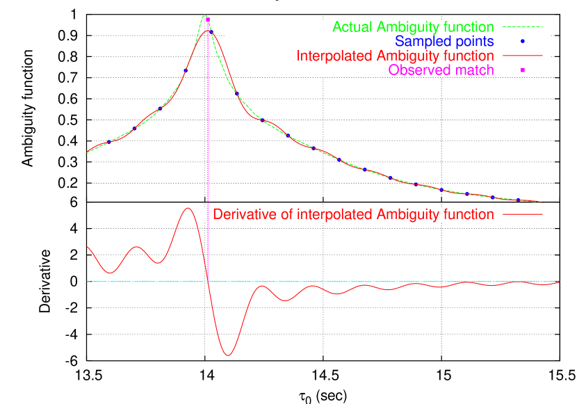
We illustrate the interpolated search strategy using Fig. 1. In Fig. 1 we use $37$ interpolating search templates, that is, we sample the ambiguity function at $37$ points in the $\tau_{0}$ space (the marked points on the dotted curve). We construct the interpolating function (the solid curve) and find its maximum by setting its derivative to zero. In order to avoid local extrema, we first find the approximate location of the peak of the interpolating function and then find the zero of its derivative by successive approximation near the region of the peak. One can clearly see that the proper value of the ambiguity function at the maximum of the interpolating function is more than the maximum value of the interpolating function and this is what we gain by placing a template at the maximum of the interpolating function.

III.2 A one-dimensional parameter space for comparative studies

We are interested in understanding the performance of the interpolated search strategy relative to the dense search strategy, which is currently used in the analysis of data from the LIGO, GEO and TAMA detectors Abbott et al. (2004b). The current analyses focus on templates corresponding to binaries with circular orbits and no component spins. The corresponding two-dimensional parameter space is spanned by the masses of the individual components. The templates vary most rapidly, however, along the axis spanned by the so-called chirp mass

$$\mathcal{M}:=\mu^{3/5}M^{2/5},$$ (26)

where $M$ is the system’s total mass and $\mu$ its reduced mass. The linear density of templates needed by the dense search in the direction $\partial_{\mathcal{M}}$ is approximately 100 times the linear density needed in the orthogonal direction. For the comparison we perform here we focus attention on the number of template evaluations needed for binaries with equal mass components that vary only in $\mathcal{M}$. We expect that the ratio of performance, measured as the number of templates required by the two search strategies to achieve the same search results, will be the same in the complementary dimension and in the other dimensions that will be introduced in future searches that accommodate component spins and orbital eccentricity.

III.3 Templates

The strain response of an interferometric gravitational wave detector to quadrupole formula approximation gravitational waves incident from an inspiraling binary neutron star system can be written

$$h(t|t_{a},\tau_{0})=h_{0}\left[\pi f(t-t_{a}-\tau_{0})\mathcal{M}\right]^{2/3}\cos\Phi(t-t_{a}-\tau_{0}),$$ (27a)

where

$$f(t|t_{a},\tau_{0}) := \dfrac{1}{\pi\mathcal{M}}\left(\dfrac{5}{256}\dfrac{\mathcal{M}}{\tau_{0}+t_{a}-t}\right)^{3/8},$$ (27b)

$$\Phi(t|t_{a},\tau_{0}) := \Phi_{a}+2\pi\int_{t}^{t_{a}+\tau_{0}}dt\,f(t|t_{a},\tau_{0})$$ (27c)

for $t<t_{a}+\tau_{0}$. Here $t_{a}$ is the moment when the instantaneous wave frequency is equal to $f_{a}$ and $\tau_{0}$ is the elapsed time from that moment until (in this approximation) the system coalesces, which is directly related to the system’s chirp mass $\mathcal{M}$:

$$\tau_{0}=\dfrac{5}{256\pi f_{a}}\dfrac{1}{\left(\pi\mathcal{M}f_{a}\right)^{5/3}}.$$ (28)

The elapsed time to coalescence $\tau_{0}$ is a useful surrogate for the chirp mass $\mathcal{M}$: templates equispaced in $\tau_{0}$ have constant cross-correlation, independent of $\tau_{0}$. Choosing $f_{a}$ equal to 40 Hz, which is commonly taken as the lower-edge of the LIGO detector bandwidth at design sensitivity Lazzarini and Weiss (1995), $\tau_{0}$ ranges from approximately 43 s for a binary system consisting of two $1\,\text{M}_{\odot}$ compact objects to 0.15 s for a binary consisting of two $30\,\text{M}_{\odot}$ black holes.

It is convenient to work with the Fourier transform of the strain response of the detector. For neutron star binaries in the LIGO or Virgo band the Fourier transform can be evaluated to an excellent approximation using the stationary phase approximation Finn and Chernoff (1993):

$$\tilde{h}(f)=\mathcal{N}f^{-7/6}\exp\left\{i\left[-\Phi_{a}-\pi/4+\Psi(f|t_{a},\tau_{0})\right]\right\},$$ (29a)

where

$$\Phi_{a} = \Phi(t_{a}|t_{a},\tau_{0}),$$ (29b)

$$\Psi(f|t_{a},\tau_{0}) = 2\pi ft_{a}+f_{a}\tau_{0}\dfrac{6\pi}{5}\left(\dfrac{f}{f_{a}}\right)^{-5/3}.$$ (29c)

The factor $\mathcal{N}$ is a constant amplitude.

It is important to distinguish between the nature of the parameters that characterize the template. Changes in the parameter $\tau_{0}$ change the waveform shape: we term such parameters dynamical parameters. On the other hand, parameters such as $t_{a}$ or $\Phi_{a}$ translate the waveform, but do not alter its shape: we term these kinematical parameters. In our problem only the subspace of dynamical parameters needs to be spanned by discrete templates: the values of the kinematic parameters for the Wiener filter with the maximum output can be determined by other means. Correspondingly, at the level of approximation associated with the quadrupole formula the family of templates that must be evaluated is one dimensional.

III.4 Dense search template placement

There are many different ways of parameterizing the template space. Choosing $\tau_{0}$ as a dynamical variable has the advantage that $\Gamma(\tau_{0},\tau^{\prime}_{0})$ depends only on the difference $\tau_{0}-\tau^{\prime}_{0}$; consequently, in the dense search templates are spaced uniformly in $\tau_{0}$ Sathyaprakash and Dhurandhar (1991); Dhurandhar and Schutz (1994); Owen (1996). To determine that spacing we evaluate

$$\mathcal{H}(\Delta\tau_{0})=\Gamma(\tau_{0},\tau_{0}+\Delta\tau_{0}),$$ (30)

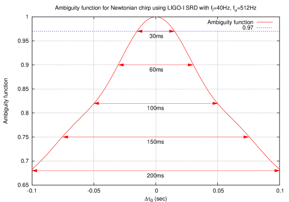
where now $\Gamma$ has been maximized over the kinematical parameters $t_{a}$ and $\phi_{a}$. This maximization can be performed in a computationally efficient manner as shown in the literature Sathyaprakash and Dhurandhar (1991). We call $\mathcal{H}$ the dynamical ambiguity function or simply as the ambiguity function. It quantifies the fractional match between the template at $\tau_{0}$ and the signal at $\tau_{0}+\Delta\tau_{0}$. Figure 2 shows $\mathcal{H}$ for power spectral density specified in the initial LIGO science requirements Lazzarini and Weiss (1995). The requirement that $\mathcal{H}(\Delta\tau_{0})$ is equal to a constant for any two consecutive templates determines the spacing $\Delta\tau_{0}$ between templates that differ only in $\tau_{0}$. For our example problem, which has just one dynamical parameter, the requirement that $\mathcal{H}(\Delta\tau_{0})$ is 97% (the conventional choice) for neighboring templates leads to a template spacing $\Delta\tau_{0}$ equal to 30 ms.

Figure 2: Ambiguity function ${\cal H}$ plotted as a function of $\Delta\tau_{0}$. Horizontal lines are drawn for various matches; the dotted horizontal line is for a 97% match, which corresponds to an inter-template separation of $\sim 30$ ms.

III.5 Interpolated search template placement

In the dense search templates are equispaced in $\tau_{0}$, with the spacing between adjacent templates — and thus the number of templates — chosen such that the dynamical ambiguity function takes on a specified value. When presented with data an event is signaled when the amplitude at one of these templates exceeds a threshold.

In the interpolated search, on the other hand, the domain $[\tau_{0}^{\min},\tau_{0}^{\max}]$ is mapped onto $[-1,1]$ and the placement and number of templates is chosen to simplify the construction of the Chebyshev interpolating polynomial of the template output over this domain. When presented with data the maximum value of the Chebyshev interpolating polynomial is found and an event is signaled when the amplitude at that location exceeds a threshold.

In the interpolated search our goal is to minimize the order of the interpolating polynomial (and, thus, the number of template evaluations) required for a given accuracy of interpolation. We have some control over this through the choice of mapping from $[\tau_{0}^{\min},\tau_{0}^{\max}]$ to $[-1,1]$. The linear map

$$\tau^{\prime}=2\dfrac{\tau_{0}-\tau_{0}^{\min}}{\tau_{0}^{\max}-\tau_{0}^{\min}}-1,$$ (31)

is the most obvious such mapping. While have not made an exhaustive search of all possible mappings; however, we have observed that better fits are possible with a lower-order polynomial when we use the mapping

$$\delta=-\cos\left[\pi\,\dfrac{\tau_{0}-\tau_{0}^{\min}}{\tau_{0}^{\max}-\tau_{0}^{\min}}\right].$$ (32)

Moreover, with this mapping, the roots of the Chebyshev polynomial are equi-spaced over the parameter range in $\tau_{0}$. Once we have fixed the order $n$ of the interpolating polynomial templates are placed at values of $\delta$ that are roots of the $T_{n+1}(\delta)$ and the coefficients of the interpolating polynomial are found using equation 23.

Figure 3: Normalized test signals (without noise) were injected densely at regular intervals along the parameter space and the match obtained by the interpolated search strategy is plotted against $\tau_{0}$. This figure demonstrates that the match is a (nearly) periodic function of $\tau_{0}$ with the period equal to the template separation. Moreover, with just $37+1$ interpolated search templates the minimal match is $0.97$. For the same minimal match $133$ templates are needed for the usual dense search.

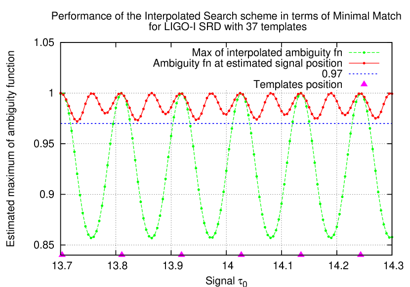
In Fig. 3 we have plotted the match by placing normalized test signals (without noise) at regular intervals of $\tau_{0}$. We see that the match is a (nearly) periodic function of $\tau_{0}$, with the period equal to the template separation. This suggests that the detection probability is also periodic and this fact has been used in carrying out the simulations - the signals are injected within one such “period” in the parameter space. Moreover, one can see that with just $37+1$ interpolated search templates one gets a minimal match of $0.97$, whereas the dense search requires about $133$ templates to achieve the same level of minimal match. This amounts to a factor of $3.5$ over the dense search and this is so for just one dimension.

III.6 Comparison

We are interested in two, related, comparisons: first, the relative “sensitivity” of a search carried-out with a fixed number of template evaluations using the dense search strategy and the interpolated search strategy; second, the number of template evaluations required by the interpolated search in order to achieve the same “sensitivity” as the dense search. To give meaning to the “sensitivity” of these two strategies we use the Receiver Operating Characteristic, or ROC.

The ROC is a plot of true positives as a function of the fraction of false positives for a binary classifier system as its discrimination threshold is varied. Both the dense search and the interpolated search are binary classifiers: i.e., they classify an interval of data $\mathbf{d}$ as including a signal or not including a signal. A true positive is a classification of $\mathbf{d}$ as including a signal when in fact it does; a false positive is a classification of $\mathbf{d}$ as including a signal when it does not. In both of the search strategies described here the discrimination threshold is matched filter output that must be exceeded for a data interval to be classified as including a signal. The false positive fraction is also known as the type II, or false alarm, error fraction and is denoted $\alpha$. The fraction of true positives is also known as the detection efficiency $\epsilon$, which is one minus the type I, or false positive, error fraction (which is denoted $\beta$). At fixed $\alpha$ a more sensitive search method has a greater $\epsilon$. The ROC associated with a search method no better than a toss of a (possibly loaded) coin is given by the diagonal $\alpha=\epsilon$.

Using numerical simulations we have evaluated $\alpha$ and $\epsilon$ as a function of the detection threshold for both the interpolated search and the dense search, for different numbers of templates (dense search) and different interpolating polynomial order (interpolated search).

To evaluate the false positive fraction $\alpha$ we generate a large number of data segments, each $2^{15}$ samples long, and each consisting of Gaussian noise whose power spectrum (assuming a 1024 Hz sample rate) is that specified as the initial LIGO science requirement Lazzarini and Weiss (1995). (The Gaussian random numbers are themselves generated using the Mersenne Twister Pseudo Random Number Generator Matsumoto and Nishimura (1998) and then filtered in the Fourier domain by scaling the Fourier components by the square root of the PSD.) For the purpose of this comparison we look for signals in the interval $\tau_{0}\in[13\,\text{s},17\,\text{s}]$. Both the dense and interpolated search methods are applied to this data. The ratio of the number of events signaled to the number of data segments examined as a function of the threshold $\eta$ is $\alpha$ for that threshold. Approximately 50,000 realizations of detector noise are used to evaluate $\alpha$, which gives reliable results for $\alpha$ greater than approximately $10^{-3}$.

To compute $\epsilon$, the true positive fraction, we proceed in a similar fashion. Now, however, with each noise instantiation we add a signal, with $\tau_{0}$ drawn uniformly and randomly from the interval covered by the search: i.e., $\tau_{0}\in[13\,\text{s},17\,\text{s}]$. In almost all cases $50,000$ realizations of detector noise plus signal are used to evaluate the efficiency, which gives reliable results for efficiencies greater than approximately $10^{-3}$. However, for the flat search with $40$ templates and the interpolated search with $30$ templates,we have used $400,000$ realizations. The larger number of realizations in these cases results in smoother curves.

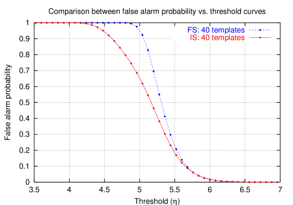
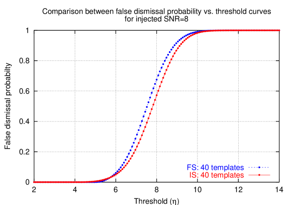
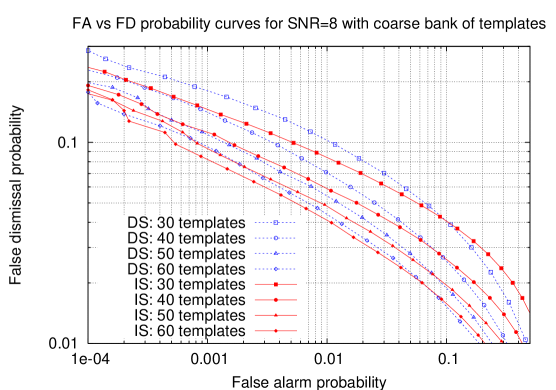
The top panel of Fig. 4 shows the variation of $\alpha$ for both methods using $40$ templates: i.e., a 100 ms template spacing for the dense search and an order 39 interpolating polynomial in $\delta$ (cf. equation 32). For any threshold $\alpha$ is always greater for the dense search than for the interpolated search; similarly, as shown in the center panel of Fig. 4, for any given threshold the efficiency $\epsilon$ is always greater for the interpolated search than for the dense search. Finally, the bottom panel of Fig. 4 shows the ROC for a 40 template dense search and an order 39 interpolated search, both of which involve 40 template evaluations to decide if a signal has been detected. Comparing both ROCs it is clear that the interpolated search is more sensitive at any given $\alpha$ then the dense search. This is always true: i.e., for a fixed number of template evaluations the interpolated search will always have a better efficiency at a given $\alpha$ than the dense search, though as the number of templates grows large the fractional difference in sensitivity will decrease.

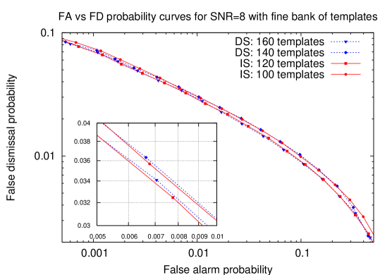
Figure 5 and table I addresses the second of our two questions: the number of templates evaluations required of an interpolated search to have the same sensitivity as a dense search. Figure 5 shows the ROCs for dense searches using 140 and 160 templates, together with the ROCs for interpolated searches using 120 and 100 templates. The interpolated search with and order 120 interpolating polynomial is clearly as sensitive as a dense search with 160 templates, and an interpolating search with an order 100 polynomial is as sensitive as a dense search with 140 templates. Table I shows similar pairings of the number of templates in a dense search and the number of templates in an interpolating search necessary to achieve the same sensitivity.

Figure 4: The variation of the false and true positive fractions, $\alpha$ and $\epsilon$ with threshold $\eta$ for the dense and interpolated search methods, each making use of 40 template evaluations. The top panel shows the false positive fraction. Note how the false positive falls much sooner for the interpolated search than for the dense search. The bottom panel shows $\epsilon$ when a signal of amplitude signal to noise 8 is present in the range $\tau_{0}\in[13\,\text{s},17\,\text{s}]$. Note how the $\epsilon$ is always greater for the interpolated search than for the dense search. For the same computational cost (determined by the number of template evaluations) the interpolated search will always perform better than the dense search.

Figure 5: ROC curves for dense searches (solid curves) and interpolating searches (dashed curves). For a given number of templates, the solid curves are ‘lower’ - less false dismissal probability for the same false alarm - than the dotted curves in the regime of low false alarm showing that the interpolated search performs better than the dense search for low false alarm. The bottom panel shows analogous plot for high minimal match (fine bank) $\sim.98$. Here the performance of the dense search with 160 and 140 templates is comparable to that of the interpolated search with 120 and 100 templates respectively.

Table 1: Number of template evaluations required to obtain the same efficiency at a false alarm fraction of $10^{-3}$ in a dense search and an interpolated search. Note how the interpolated search is computational more efficient for the same sensitivity.

# templates		$\epsilon$ at $\alpha=10^{-3}$
Dense	Interp.
40	31	0.859
50	41	0.890
60	49	0.905
80	64	0.919
100	89	0.924
140	105	0.927
160	115	0.929

IV Conclusion

We have shown that the use of near-minimax interpolating polynomials to fit the output of matched filters to the filter parameter values can greatly improved the sensitivity of a matched-filter based search for gravitational waves from compact binary inspiral. Using such a polynomial to find the parameters of the signal template leading to the best match we can reduce the computational cost of a search over a two dimensional parameter space by a factor of two compared to the methods currently in use, without any loss of sensitivity or discriminating power. This factor of two becomes a factor of ten when the search is over the seven dimensional parameter space that includes not only the masses but also the spins of the binary components Buonanno et al. (2004). This savings in computational cost is estimated under the assumption, which we believe well-founded, that we will obtain the same savings when the interpolation is extended to additional dimensions.

The use of near-minimax interpolation should be considered as part of a larger strategy that employs a multi-grid approach to determine whether a signal has been observed and, if so, the parameters that characterize it. Since the major contribution to the computational cost of a multi-grid search is thought to arise in the initial stage of the search the gain in computational efficiency — and, correspondingly, the size of the parameter space that can studied with fixed computational resources — could be substantial.

References

- Sanders (2003) G. H. Sanders, in Gravitational-Wave Detection. Edited by Cruise, Mike; Saulson, Peter. Proceedings of the SPIE, Volume 4856, pp. 247-257 (2003). (2003), pp. 247–257.
- Abbott et al. (2004a) B. Abbott, R. Abbott, R. Adhikari, A. Ageev, B. Allen, R. Amin, S. B. Anderson, W. G. Anderson, M. Araya, H. Armandula, et al., Physical Review D 69 (2004a), iSI Document Delivery No.: 838AA Times Cited: 7 Article 122004.
- Ando and Tsubono (2000) M. Ando and K. Tsubono, in Gravitational Waves, edited by S. Meshkov (American Institute of Physics, Melville, New York, 2000), no. 523 in AIP Conference Proceedings, proceedings of the Third Edoardo Amaldi Conference.
- Acernese et al. (2003) F. Acernese, P. Amico, N. Arnaud, D. Babusci, G. Ballardin, R. Barillé, F. Barone, M. Barsuglia, F. Beauville, F. Bellachia, et al., Classical and Quantum Gravity 20, S609 (2003).
- Blanchet et al. (1995) L. Blanchet, T. Damour, and B. R. Iyer, Phys. Rev. D 51, 5360 (1995).
- Damour et al. (2001) T. Damour, B. R. Iyer, and B. S. Sathyaprakash, Phys. Rev. D 63, 044023 (2001).
- Damour et al. (2002) T. Damour, B. R. Iyer, and B. S. Sathyaprakash, Phys. Rev. D 66, 027502 (2002).
- Finn (1992) L. S. Finn, Phys. Rev. D 46, 5236 (1992).
- Finn and Chernoff (1993) L. S. Finn and D. F. Chernoff, Phys. Rev. D 47, 2198 (1993).
- Abbott et al. (2004b) B. Abbott, R. Abbott, R. Adhikari, A. Ageev, B. Allen, R. Amin, S. B. Anderson, W. G. Anderson, M. Araya, H. Armandula, et al., Physical Review D 69 (2004b), iSI Document Delivery No.: 838AA Times Cited: 12 Article 122001.
- Sathyaprakash and Dhurandhar (1991) B. S. Sathyaprakash and S. V. Dhurandhar, Phys. Rev. D 44, 3819 (1991).
- Dhurandhar and Schutz (1994) S. V. Dhurandhar and B. F. Schutz, Phys. Rev. D 50, 2390 (1994).
- Croce et al. (2000a) R. P. Croce, T. Demma, V. Pierro, I. M. Pinto, D. Churches, and B. S. Sathyaprakash, Phys. Rev. D 62, 121101 (2000a).
- Croce et al. (2000b) R. P. Croce, T. Demma, V. Pierro, I. M. Pinto, and F. Postiglione, Phys. Rev. D 62, 124020 (2000b).
- Mohanty and Dhurandhar (1996) S. D. Mohanty and S. V. Dhurandhar, Phys. Rev. D 54, 7108 (1996).
- Mohanty (1998) S. D. Mohanty, Phys. Rev. D 57, 630 (1998).
- Croce et al. (2004a) R. P. Croce, T. Demma, M. Longo, S. Marano, V. Matta, V. Pierro, and I. M. Pinto, Phys. Rev. D 70, 122001 (2004a).
- Croce et al. (2004b) R. P. Croce, T. Demma, M. Longo, S. Marano, V. Matta, V. Pierro, and I. M. Pinto, Classical and Quantum Gravity 21, 4955 (2004b).
- Sengupta et al. (2003) A. S. Sengupta, S. Dhurandhar, and A. Lazzarini, Phys. Rev. D 67, 082004 (2003).
- Shannon (1949) C. E. Shannon, Proc. Inst. Radio Eng. 37, 10 (1949).
- Mason and Handscomb (2003) J. C. Mason and D. C. Handscomb, Chebyshev polynomials (Chapman & Hall/CRC, Boca Raton, 2003).
- Powell (1967) M. J. D. Powell, The Computer J. 9, 404 (1967).
- Li (2004) R.-C. Li, IEEE Trans. Comp. 53, 678 (2004).
- Owen (1996) B. J. Owen, Phys. Rev. D D53, 6749 (1996).
- Lazzarini and Weiss (1995) A. Lazzarini and R. Weiss, Tech. Rep. LIGO-E950018-02-E, Laser Interferometer Gravitational Wave Observatory (1995), internal working note.
- Matsumoto and Nishimura (1998) M. Matsumoto and T. Nishimura, ACM Trans. on Modeling and Computer Simulation 8, 3 (1998).
- Buonanno et al. (2003) A. Buonanno, Y. Chen, and M. Vallisneri, Phys. Rev. D 67, 104025 (2003).
- Buonanno et al. (2004) A. Buonanno, Y. Chen, Y. Pan, and M. Vallisneri, Phys. Rev. D 70, 104003 (2004).