Multi-block simulations in general relativity: high order discretizations, numerical stability, and applications

Luis Lehner1, Oscar Reula2, and Manuel Tiglio1,3,4 111 Department of Physics and Astronomy, Louisiana State University, Baton Rouge, LA 70803-4001
222 FaMAF, Universidad Nacional de Cรณrdoba, Ciudad Universitaria, 5000 Cรณrdoba, Argentina
333 Center for Computation and Technology, 302 Johnston Hall, Louisiana State University, Baton Rouge, LA 70803-4001
444 Center for Radiophysics and Space Research, Cornell University, Ithaca, NY 14853
Abstract

The need to smoothly cover a computational domain of interest generically requires the adoption of several grids. To solve the problem of interest under this grid-structure one must ensure the suitable transfer of information among the different grids involved. In this work we discuss a technique that allows one to construct finite difference schemes of arbitrary high order which are guaranteed to satisfy linear numerical and strict stability. The technique relies on the use of difference operators satisfying summation by parts and penalty techniques to transfer information between the grids. This allows the derivation of semidiscrete energy estimates for problems admitting such estimates at the continuum. We analyze several aspects of this technique when used in conjuction with high order schemes and illustrate its use in one, two and three dimensional numerical relativity model problems with non-trivial topologies, including truly spherical black hole excision.

I Introduction

Many systems of interest have a non-trivial natural topology that a single cubical computational domain cannot accommodate in a smooth manner. Examples of these topologies in three-dimensional settings are S2ร—Rsuperscript๐‘†2๐‘…S^{2}\times R (or a subset of it), encountered when dealing with spacetimes with smooth outer boundary and inner boundaries where required to excise singularities, and S2ร—S1superscript๐‘†2superscript๐‘†1S^{2}\times S^{1} or S3superscript๐‘†3S^{3} topologies, commonly found in cosmological problems.

The need to treat these scenarios naturally leads one to consider multiple coordinate patches in order to cover the region of integration. These, in turn, translate into having to adopt multiple grids at the implementation level. Each one of these represents a region of discrete space, a patch, which might come equipped with a discrete Cartesian coordinate system or discrete charts; that is, invertible maps from discrete space to regions of Z3superscript๐‘3Z^{3} (i.e. the integers labeling coordinate grid points in each direction).

Covering a spacetime by charts is commonly done at the continuum level when considering the differential geometry of the spacetime (see for instance wald ). These charts are usually thought of as defining a map of a portion of the spacetime into a subset of R3superscript๐‘…3R^{3}, and the combination of charts (which usually overlap in some regions) covers the whole spacetime. Points belonging to an overlapping region are considered as belonging to any of the involved charts. Here a well defined coordinate transformation between the charts is naturally defined by the combination of the maps and their inverse in between the spacetime and the charts.

At the discrete level one can in principle adopt an analog of the above construction. However, it is often the case that in the overlapping region a grid point in one of the charts does not have a corresponding one in the other. Consequently, the coordinate transformation is not defined. This presents a problem at the practical level as communication between patches must take place. This issue is commonly solved in two different ways: (I) By introducing further points via interpolation where needed, (II) By considering patches that only abut, i.e. do not overlap.

In the first case โ€“ commonly referred to as overlapping-grids approach โ€“ non-existent points in a given grid within the overlapping region are defined where needed by appropriate interpolations. Although this can be done in a straightforward manner with a relatively simple multiple-grid structure, the drawback of this approach is the introduction of a new ingredient โ€“ the interpolation โ€“ which does not have a counterpart at the continuum. This complicates the assessment of stability of even simple evolution problems as the details of the interpolation itself are intertwined with any attempt in this direction in an involved manner. As a consequence, there exist few stability proofs for such evolution schemes and have so far been restricted to one-dimensional settings. Notwithstanding this point a number of implementations in Numerical Relativity, where the possible truncation-error driven inconsistencies at the interfaces are dealt with by introducing a certain amount of dissipation or filtering, make use of this approach with good results (see for instance, overlapping1 ; overlapping2 ; overlapping3 ; overlapping4 ).

In the second case โ€“ commonly referred to as multi-block approach โ€“ grids are defined in a way such that there is no overlap and only grid points at boundaries are common to different grids. This requirement translates into having to define the multiple grids with greater care than in the previous option. This extra effort, however, has as one pay off that schemes preserving important continuum properties can be constructed. In particular, this allows the construction of stability analyses which are similar to those of a single grid. More explicitly, following Abarbanel, Carpenter, Nordstrom, and Gottlieb penalties0 ; penalties1 ; penalties2 one can construct schemes of arbitrary high order for which semi-discrete energy estimates are straightforward to derive in a general way. The availability of stability results for this second approach makes it a very attractive option in involved problems โ€“like those typically found when evolving Einstein equationsโ€“ where schemes eliminating spurious sources of instabilities provide a strong starting point for a stable implementation of the problem.

In this paper we discuss and analyze the use of this multi-block approach in the context of Numerical Relativity. At the core of the technique to treat outer and patch interfaces is the addition of suitable penalty terms to the evolution equations penalties0 ; penalties1 ; penalties2 . In the case of hyperbolic systems these terms penalize the possible mismatches between the different values the characteristic fields take at the interface between several patches.

Not only does this method provide a consistent way to communicate information between the different patches but, more importantly, does so in a way which allows for the derivation of energy estimates at the semi-discrete level. Consequently, numerical stability can be ensured for a large set of problems. These estimates can be obtained with difference operators of any accuracy order, provided they satisfy the summation by parts (SBP) property and the penalty terms are constructed appropriately.

In this work we discuss this technique in a context relevant to numerical relativity, analyze its properties and illustrate it in specific examples. In particular we show results for the case of the S2ร—Rsuperscript๐‘†2๐‘…S^{2}\times R topology used in black hole excision techniques.

This work is organized as follows. Section II includes a description of the numerical analysis needed to attain stability in the presence of multiple grids and summarize how the penalty method of Refs. penalties0 ; penalties1 ; penalties2 allows for achieving this goal.

In Section III we study some aspects of Strandโ€™s strand high order operators satisfying SBP with respect to diagonal norms, when combined with the penalty technique. We find that in some cases, typically used operators that minimize the bandwidth have a very large spectral radius, with corresponding limitations in the Courant-Friedrich-Levy (CFL) factor when used in evolution equations. We therefore construct operators that minimize the spectral radius instead. Additionally, we examine the behavior of the convergence rate and the propagation behavior that different modes have when employing different higher order operators.

In Section IV we present and analyze different tests relevant to numerical relativity employing derivative operators of different order of accuracy and the penalty technique to deal with multiple grids. These tests cover from linearized Einstein equations (in effectively one-dimensional scenarios) to propagation of three-dimensional fields in curved backgrounds.

We defer to appendices the discussion of several issues. Appendix A presents details of the higher derivative operators and diagonal norms which we employ in this work. Appendix B discusses our construction of high order dissipative operators which are negative definite with respect to the corresponding SBP scalar product. Last, Appendix C lists some useful properties that finite difference derivative operator satisfy, which help in our construction of dissipative operators.

II Interface treatment for symmetric hyperbolic problems in multiple blocks

As mentioned, we are interested in setting up a computational domain which consists of several grids which just abut. This domain provides the basic arena on which symmetric hyperbolic systems are to be numerically implemented. The basic strategy is to discretize the equations at each individual grid or block, treating boundary points in a suitable way. Boundary points at each grid either represent true boundary ones from a global perspective or lie at the interface between grids. In the latter case, since these points are common to more than one grid the solution at them can be regarded as multi-valued. As we show below, this issue can be dealt with consistently and stably, ensuring that any possible mismatch converges to zero with resolution.

At the core of the technique is the appropriate communication of these possibly different values of the solution at the interfaces. Intuitively, since we are dealing with symmetric hyperbolic systems, a natural approach would be to communicate the characteristic variables from one domain to the other one. However, this is not known to be numerically stable. There exists nonetheless a technique based on this strategy which does guarantee numerical stability penalties0 ; penalties1 ; penalties2 . This relies in adding penalty terms to the evolution equations of characteristic fields which penalize: a) in the interface case the mismatch between the different values each characteristic field takes at the interface of several grids; b) in the outer boundary case the difference between each incoming characteristic field and the boundary conditions one wishes to impose to it.

These penalty terms are constructed so as to guarantee the stability of the whole composite grid if it can be guaranteed at each individual grid through the energy method. To this end, the use of schemes with difference operators satisfying SBP are employed. Hence, on each single grid there exists a family of natural semidiscrete energies, defined by both a symmetrizer of the continuum equations and a discrete scalar product with respect to which SBP holds 111Symmetrizers are not unique, already at the continuum level. In the case in which there is a preferred one there is, similarly, a single, preferred semidiscrete energy on each grid. This is the case, for example, when one can derive a sharp energy estimate at the continuum, which gives rise to the construction of a strictly stable scheme, see strict for a detailed discussion in the context of Numerical Relativity.. One can then define an energy for the whole domain by simply adding the different energies of each grid. The use of operators satisfying SBP allows one to get an energy estimate, up to outer boundary and interface terms left after SBP. The penalties allow to control their contribution, thus obtaining an estimate for the global grid. This is achieved if the contribution to the time derivative of the energy due to the interface and outer boundary terms (in the latter case when, say, homogenous maximally dissipative outer boundary conditions are imposed) left after SBP is non-positive. When these terms are exactly zero the penalty treatment of Refs. penalties0 ; penalties1 ; penalties2 is, in a precise sense, โ€œenergy non-dissipativeโ€. On the other hand, if these terms are negative the scheme is numerically stable but at fixed resolution a damping of the energy (with respect to the growth one would obtain in the absence of an interface) in time arises. This damping is proportional to either the mismatch of a given characteristic variable at each interface or its failure to satisfy an outer boundary condition. As we describe below, these interface and boundary terms left after SBP are controlled precisely by the mentioned penalties, each of which depends on: the possible mismatch; the characteristic speeds, the corresponding SBP scalar product at the interface, the resolution at each intervening grid, and a free parameter which regulates the strength of the penalties.

Next, we explicitly describe how this penalty technique allows one to derive semidiscrete energy estimates. We first discuss in detail the one-dimensional example of an advection equation on a domain with a single interface. The more general case of systems of equations in several dimensions follows essentially the same principles, applying the 111d treatment to each characteristic field. We illustrate this by discussing a general constant-coefficient system in a given two-dimensional setting. From this, the generalization to the three-dimensional general case is straightforward, and we therefore only highlight its salient features.

II.1 A one-dimensional example

Consider a computational domain represented by a discrete grid consisting of points i=imโ€‹iโ€‹nโ€‹โ€ฆโ€‹imโ€‹aโ€‹x๐‘–subscript๐‘–๐‘š๐‘–๐‘›โ€ฆsubscript๐‘–๐‘š๐‘Ž๐‘ฅi=i_{min}\ldots i_{max} and gridspacing hโ„Žh covering xโˆˆ[a,b]๐‘ฅ๐‘Ž๐‘x\in[a,b]. A 111d difference operator D๐ทD on such a domain is said to satisfy SBP with respect to a positive definite scalar product (defined by its coefficients ฯƒiโ€‹jsubscript๐œŽ๐‘–๐‘—\sigma_{ij})

โŸจu,vโŸฉ=hโ€‹โˆ‘i,juiโ€‹vjโ€‹ฯƒiโ€‹j,๐‘ข๐‘ฃโ„Žsubscript๐‘–๐‘—subscript๐‘ข๐‘–subscript๐‘ฃ๐‘—subscript๐œŽ๐‘–๐‘—\langle u,v\rangle=h\sum_{i,j}u_{i}v_{j}\sigma_{ij}\,, (1)

if the property

โŸจu,Dโ€‹vโŸฉ+โŸจv,Dโ€‹uโŸฉ=(uโ€‹v)|ab๐‘ข๐ท๐‘ฃ๐‘ฃ๐ท๐‘ขevaluated-at๐‘ข๐‘ฃ๐‘Ž๐‘\langle u,Dv\rangle+\langle v,Du\rangle=\left(uv\right)|_{a}^{b}

holds for all gridfunctions u,v๐‘ข๐‘ฃu,v. The scalar product/norm is said to be diagonal if ฯƒiโ€‹j=ฯƒiโ€‹iโ€‹ฮดi,jsubscript๐œŽ๐‘–๐‘—subscript๐œŽ๐‘–๐‘–subscript๐›ฟ๐‘–๐‘—\sigma_{ij}=\sigma_{ii}\delta_{i,j}222Here ฮดi,jsubscript๐›ฟ๐‘–๐‘—\delta_{i,j} is the Kronecker delta (ฮดi,j=1subscript๐›ฟ๐‘–๐‘—1\delta_{i,j}=1 if i=j๐‘–๐‘—i=j and zero otherwise). One advantage of 111d difference operators satisfying SBP wrt diagonal norms is that SBP is guaranteed to hold in several dimensions if the 111d operator is used on each direction (which is not known to hold in the non-diagonal case in general) olsson . Even in 111d, in the variable coefficients and non-diagonal case the commutator between D๐ทD and the principal part might not be bounded for all resolutions (something that is generically 333That is, unless the scheme can be written in strictly stable form. needed for an energy estimate to hold) svard . Another advantage is that the operators are, for a given order in the interior, simpler in their expressions. The disadvantage is that their order at and close to boundaries is half that one in the interior, while in the non-diagonal case the operators loose only one order with respect to the interior sbp_order ; strand . Throughout this paper we will mostly restrict our treatment to the use of diagonal norms.

As an example of how to impose interface or outer boundary conditions through penalty terms, we concentrate next on the advection equation for u๐‘ขu propagating with speed ฮ›ฮ›\Lambda,

uห™=ฮ›โ€‹โˆ‚xu.ห™๐‘ขฮ›subscript๐‘ฅ๐‘ข\dot{u}=\Lambda\partial_{x}u\;. (2)

II.1.1 A domain with an interface

Consider the interval (โˆ’โˆž,โˆž)(-\infty,\infty) with appropriate fall-off conditions at infinity. We consider two grids: a left one covering (โˆ’โˆž,0]0(-\infty,0], and a right one covering [0,โˆž)0[0,\infty). We refer to the gridfunction u๐‘ขu on each grid by ulsuperscript๐‘ข๐‘™u^{l} and ursuperscript๐‘ข๐‘Ÿu^{r} (corresponding to the left and right grids, respectively). Both of these gridfunctions have a point defined at the x=0๐‘ฅ0x=0 interface and they need not coincide there, except at the initial time. Therefore, the numerical solution will in principle be multivalued at x=0๐‘ฅ0x=0, though, as we shall see, the penalty technique is designed to keep this difference small.

The problem is discretized using on the right and left grids, respectively, with gridspacings hl,hrsuperscriptโ„Ž๐‘™superscriptโ„Ž๐‘Ÿh^{l},h^{r} โ€“not necessarily equalโ€“ and difference operators Dl,Drsuperscript๐ท๐‘™superscript๐ท๐‘ŸD^{l},D^{r} satisfying SBP with respect to scalar products given by the weights ฯƒl,ฯƒrsuperscript๐œŽ๐‘™superscript๐œŽ๐‘Ÿ\sigma^{l},\sigma^{r} at their individual grids. That is, these scalar products are defined through

โŸจul,vlโŸฉ=hlโ€‹โˆ‘i,j=โˆ’โˆž0ฯƒiโ€‹jlโ€‹uilโ€‹vjl,โŸจur,vrโŸฉ=hrโ€‹โˆ‘i,j=0โˆžฯƒiโ€‹jlโ€‹uirโ€‹vjrformulae-sequencesuperscript๐‘ข๐‘™superscript๐‘ฃ๐‘™superscriptโ„Ž๐‘™superscriptsubscript๐‘–๐‘—0subscriptsuperscript๐œŽ๐‘™๐‘–๐‘—subscriptsuperscript๐‘ข๐‘™๐‘–subscriptsuperscript๐‘ฃ๐‘™๐‘—superscript๐‘ข๐‘Ÿsuperscript๐‘ฃ๐‘Ÿsuperscriptโ„Ž๐‘Ÿsuperscriptsubscript๐‘–๐‘—0subscriptsuperscript๐œŽ๐‘™๐‘–๐‘—subscriptsuperscript๐‘ข๐‘Ÿ๐‘–subscriptsuperscript๐‘ฃ๐‘Ÿ๐‘—\langle u^{l},v^{l}\rangle=h^{l}\sum_{i,j=-\infty}^{0}\sigma^{l}_{ij}u^{l}_{i}v^{l}_{j}\;\;\;,\;\;\;\langle u^{r},v^{r}\rangle=h^{r}\sum_{i,j=0}^{\infty}\sigma^{l}_{ij}u^{r}_{i}v^{r}_{j}

The semidiscrete equations are written as

uห™ilsubscriptsuperscriptห™๐‘ข๐‘™๐‘–\displaystyle\dot{u}^{l}_{i} =\displaystyle= ฮ›โ€‹Dlโ€‹uil+ฮดi,0โ€‹Slhlโ€‹ฯƒ00lโ€‹(u0rโˆ’u0l),ฮ›superscript๐ท๐‘™subscriptsuperscript๐‘ข๐‘™๐‘–subscript๐›ฟ๐‘–0superscript๐‘†๐‘™superscriptโ„Ž๐‘™subscriptsuperscript๐œŽ๐‘™00subscriptsuperscript๐‘ข๐‘Ÿ0subscriptsuperscript๐‘ข๐‘™0\displaystyle\Lambda D^{l}u^{l}_{i}+\frac{\delta_{i,0}S^{l}}{h^{l}\sigma^{l}_{00}}(u^{r}_{0}-u^{l}_{0})\,, (3)
uห™irsubscriptsuperscriptห™๐‘ข๐‘Ÿ๐‘–\displaystyle\dot{u}^{r}_{i} =\displaystyle= ฮ›โ€‹Drโ€‹uir+ฮดi,0โ€‹Srhrโ€‹ฯƒ00rโ€‹(u0lโˆ’u0r).ฮ›superscript๐ท๐‘Ÿsubscriptsuperscript๐‘ข๐‘Ÿ๐‘–subscript๐›ฟ๐‘–0superscript๐‘†๐‘Ÿsuperscriptโ„Ž๐‘Ÿsubscriptsuperscript๐œŽ๐‘Ÿ00subscriptsuperscript๐‘ข๐‘™0subscriptsuperscript๐‘ข๐‘Ÿ0\displaystyle\Lambda D^{r}u^{r}_{i}+\frac{\delta_{i,0}S^{r}}{h^{r}\sigma^{r}_{00}}(u^{l}_{0}-u^{r}_{0})\,. (4)

Notice in the above equations the second term on each right hand side, which constitutes the penalty added to the problem. They are defined by the possible mismatch, the grid-spacing, the inner product employed and the free parameters {Sl,Sr}superscript๐‘†๐‘™superscript๐‘†๐‘Ÿ\{S^{l},S^{r}\}, which will be determined by requiring an energy estimate to hold.

We define a natural energy for the whole domain, which is the sum of the energies for each grid (for this simple example with a trivial symmetrizer),

E:=โŸจul,ulโŸฉ+โŸจur,urโŸฉ.assign๐ธsuperscript๐‘ข๐‘™superscript๐‘ข๐‘™superscript๐‘ข๐‘Ÿsuperscript๐‘ข๐‘ŸE:=\langle u^{l},u^{l}\rangle+\langle u^{r},u^{r}\rangle\,.

Taking a time derivative of this energy, using the semidiscrete equations (3,4) and the SBP property one gets

Et=(ฮ›โˆ’2โ€‹Sl)โ€‹(u0l)2+(โˆ’ฮ›โˆ’2โ€‹Sr)โ€‹(u0r)2+2โ€‹(Sl+Sr)โ€‹u0lโ€‹u0r.subscript๐ธ๐‘กฮ›2superscript๐‘†๐‘™superscriptsubscriptsuperscript๐‘ข๐‘™02ฮ›2superscript๐‘†๐‘Ÿsuperscriptsubscriptsuperscript๐‘ข๐‘Ÿ022superscript๐‘†๐‘™superscript๐‘†๐‘Ÿsubscriptsuperscript๐‘ข๐‘™0subscriptsuperscript๐‘ข๐‘Ÿ0E_{t}=(\Lambda-2S^{l})(u^{l}_{0})^{2}+(-\Lambda-2S^{r})(u^{r}_{0})^{2}+2(S^{l}+S^{r})u^{l}_{0}u^{r}_{0}\,. (5)

In order to get an energy estimate the above interface term (i.e., the right-hand side of Eq. (5)) must be non-positive for all u0l,u0rsubscriptsuperscript๐‘ข๐‘™0subscriptsuperscript๐‘ข๐‘Ÿ0u^{l}_{0},u^{r}_{0}. It is straightforward to check that this is equivalent to the three following conditions holding:

ฮ›โˆ’2โ€‹Slฮ›2subscript๐‘†๐‘™\displaystyle\Lambda-2S_{l} โ‰ค\displaystyle\leq 00\displaystyle 0 (6)
โˆ’ฮ›โˆ’2โ€‹Srฮ›2subscript๐‘†๐‘Ÿ\displaystyle-\Lambda-2S_{r} โ‰ค\displaystyle\leq 00\displaystyle 0 (7)
(ฮ›+Srโˆ’Sl)2superscriptฮ›subscript๐‘†๐‘Ÿsubscript๐‘†๐‘™2\displaystyle(\Lambda+S_{r}-S_{l})^{2} โ‰ค\displaystyle\leq 00\displaystyle 0 (8)

From there, it is clear that we need ฮ›+Srโˆ’Sl=0ฮ›subscript๐‘†๐‘Ÿsubscript๐‘†๐‘™0\Lambda+S_{r}-S_{l}=0. And with this condition the other two become Sl+Srโ‰ฅ0subscript๐‘†๐‘™subscript๐‘†๐‘Ÿ0S_{l}+S_{r}\geq 0. There are three possibilities:

  • โ€ข

    Positive ฮ›ฮ›\Lambda: we can take

    Sl=ฮ›+ฮด,Sr=ฮด,ย withย โ€‹ฮดโ‰ฅโˆ’ฮ›2formulae-sequencesubscript๐‘†๐‘™ฮ›๐›ฟformulae-sequencesubscript๐‘†๐‘Ÿ๐›ฟย withย ๐›ฟฮ›2S_{l}=\Lambda+\delta,\;\;\;S_{r}=\delta,\;\;\;\mbox{ with }\delta\geq-\frac{\Lambda}{2} (9)

    The time derivative of the energy with this choice becomes

    Et=โˆ’(u0lโˆ’u0r)2โ€‹(ฮ›+2โ€‹ฮด)โ‰ค0subscript๐ธ๐‘กsuperscriptsuperscriptsubscript๐‘ข0๐‘™subscriptsuperscript๐‘ข๐‘Ÿ02ฮ›2๐›ฟ0E_{t}=-(u_{0}^{l}-u^{r}_{0})^{2}(\Lambda+2\delta)\leq 0
  • โ€ข

    Negative ฮ›ฮ›\Lambda: similarly, we can take

    Sr=โˆ’ฮ›+ฮด,Sl=ฮด,ย withย โ€‹ฮดโ‰ฅฮ›2formulae-sequencesubscript๐‘†๐‘Ÿฮ›๐›ฟformulae-sequencesubscript๐‘†๐‘™๐›ฟย withย ๐›ฟฮ›2S_{r}=-\Lambda+\delta,\;\;\;S_{l}=\delta,\;\;\;\mbox{ with }\delta\geq\frac{\Lambda}{2} (10)

    The corresponding time derivative of the energy with this choice becomes

    Et=(u0lโˆ’u0r)2โ€‹(ฮ›โˆ’2โ€‹ฮด)โ‰ค0subscript๐ธ๐‘กsuperscriptsuperscriptsubscript๐‘ข0๐‘™subscriptsuperscript๐‘ข๐‘Ÿ02ฮ›2๐›ฟ0E_{t}=(u_{0}^{l}-u^{r}_{0})^{2}(\Lambda-2\delta)\leq 0
  • โ€ข

    Vanishing ฮ›ฮ›\Lambda: this can be seen as the limiting case of any of the above two, and we can take

    Sl=Sr=ฮด,ย withย โ€‹ฮดโ‰ฅ0.formulae-sequencesubscript๐‘†๐‘™subscript๐‘†๐‘Ÿ๐›ฟย withย ๐›ฟ0S_{l}=S_{r}=\delta,\;\;\;\mbox{ with }\delta\geq 0\;. (11)

    Hence,

    Et=โˆ’(u0lโˆ’u0r)2โ€‹2โ€‹ฮดโ‰ค0subscript๐ธ๐‘กsuperscriptsuperscriptsubscript๐‘ข0๐‘™subscriptsuperscript๐‘ข๐‘Ÿ022๐›ฟ0E_{t}=-(u_{0}^{l}-u^{r}_{0})^{2}2\delta\leq 0

The coefficients Slsubscript๐‘†๐‘™S_{l} and Srsubscript๐‘†๐‘ŸS_{r} need not be equal, but the following symmetry is important, under the change ฮ›โ†’โˆ’ฮ›โ†’ฮ›ฮ›\Lambda\to-\Lambda we should have Slโ†’Srโ†’subscript๐‘†๐‘™subscript๐‘†๐‘ŸS_{l}\to S_{r} and vice-versa, since it transforms incoming modes to outgoing ones. This is clearly satisfied by the choice above.

Summarizing, there is a freedom in the penalty factors of Eqs.(3,4), encoded in the parameter ฮด๐›ฟ\delta, which has to satisfy ฮดโ‰ฅโˆ’|ฮ›|/2๐›ฟฮ›2\delta\geq-|\Lambda|/2. If ฮด=โˆ’|ฮ›/2|๐›ฟฮ›2\delta=-|\Lambda/2| there is no interface term in the estimate (that is, exact energy conservation in the above model), while if If ฮด>โˆ’|ฮ›/2|๐›ฟฮ›2\delta>-|\Lambda/2| there is a negative definite interface term in the estimate (which represents a damping in the energy proportional to the mismatch).

As we will see below, one proceeds similarly in the more general case of systems of equations in several dimensions. The penalty terms are applied to the evolution equation of each characteristic mode, with factors given by Eqs.(9,10,11) (where ฮ›ฮ›\Lambda in the general case is the corresponding characteristic speed).

II.1.2 A domain with an outer boundary

The penalty method also allows to treat outer boundaries in a similar way. As an example, consider again the advective equation Eq.(2), but now on the domain (โˆ’โˆž,0]0(-\infty,0], with gridpoints i=โˆ’โˆžโ€‹โ€ฆโ€‹0๐‘–โ€ฆ0i=-\infty\ldots 0. Assume ฮ›>0ฮ›0\Lambda>0; boundary conditions therefore need to be given at x=0๐‘ฅ0x=0; say uโ€‹(x=0,t)=g๐‘ข๐‘ฅ0๐‘ก๐‘”u(x=0,t)=g. The semidiscrete equations are written as

uห™isubscriptห™๐‘ข๐‘–\displaystyle\dot{u}_{i} =\displaystyle= ฮ›โ€‹Dโ€‹ui+ฮดi,0โ€‹Thโ€‹ฯƒ00โ€‹(gโˆ’u0).ฮ›๐ทsubscript๐‘ข๐‘–subscript๐›ฟ๐‘–0๐‘‡โ„Žsubscript๐œŽ00๐‘”subscript๐‘ข0\displaystyle\Lambda Du_{i}+\frac{\delta_{i,0}T}{h\sigma_{00}}(g-u_{0})\,. (12)

Defining the energy to be

E=โŸจu,uโŸฉ,๐ธ๐‘ข๐‘ขE=\langle u,u\rangle,

its time derivative is

Eห™ห™๐ธ\displaystyle\dot{E} =\displaystyle= (ฮ›โˆ’2โ€‹T)โ€‹u02+2โ€‹gโ€‹u0โ€‹T,ฮ›2๐‘‡superscriptsubscript๐‘ข022๐‘”subscript๐‘ข0๐‘‡\displaystyle(\Lambda-2T)u_{0}^{2}+2gu_{0}T\,, (14)
โ‰ค\displaystyle\leq (ฮ›โˆ’T)โ€‹u02+Tโ€‹g2.ฮ›๐‘‡superscriptsubscript๐‘ข02๐‘‡superscript๐‘”2\displaystyle(\Lambda-T)u_{0}^{2}+Tg^{2}\,. (15)

As in the interface case with positive speed [c.f. Eq.(9)], we can therefore take T=ฮ›+ฮด๐‘‡ฮ›๐›ฟT=\Lambda+\delta. For the homogeneous case, g=0๐‘”0g=0, the equality (14) holds and we have

Eห™=(ฮ›โˆ’2โ€‹T)โ€‹u02,ห™๐ธฮ›2๐‘‡superscriptsubscript๐‘ข02\dot{E}=(\Lambda-2T)u_{0}^{2}\,,

indicating that for ฮดโ‰ฅโˆ’ฮ›/2๐›ฟฮ›2\delta\geq-\Lambda/2 the energy will not increase. For the non-homogeneous case (gโ‰ 0๐‘”0g\neq 0) the inequality (15) yields

Eห™โ‰คฮ›โ€‹g2+ฮดโ€‹(g2โˆ’u02);ห™๐ธฮ›superscript๐‘”2๐›ฟsuperscript๐‘”2superscriptsubscript๐‘ข02\dot{E}\leq\Lambda g^{2}+\delta(g^{2}-u_{0}^{2})\,;

Note that for ฮด=0๐›ฟ0\delta=0 one trivially recovers the continuum estimate. For other values of ฮด๐›ฟ\delta the consistency with the continuum estimate follows from the observation that u0subscript๐‘ข0u_{0} converges to g๐‘”g to the s+1๐‘ 1s+1-th order if the SBP derivative operator has accuracy s๐‘ s at the boundary pointย olivierthanks . This implies that both the numerical implementation and the corresponding energy estimate are consistent with those defined at the continuum level.

At this point we find it important to remark the following. Notice that just having an energy inequality is not enough, as one further needs to ensure consistency of the discrete equations with respect to the continuum ones. In the case of the penalty approach this not straightforward as the penalty term diverges when the grid size decreases unless u๐‘ขu converges to g๐‘”g sufficiently fast (as mentioned above, u๐‘ขu does converge to g๐‘”g fast enough if u๐‘ขu is an incoming mode). In fact, the penalty term can be viewed at the continuum as approximating the original equation and boundary conditions through the introduction of a suitable delta function at the boundary. The argument of the delta function must be consistent with the underlying problem. For instance, if one were to put a penalty term on a boundary where the mode is outgoing โ€“and thus the value of the function there is determined by the evolution itselfโ€“ the inconsistency would manifest itself through a lack of convergence. In the above example this would be the case if we take ฮ›<0ฮ›0\Lambda<0 but insist in putting a penalty term at x=0๐‘ฅ0x=0. Note that in such situation the energy inequality would still hold if Tโ‰ฅฮ›/2๐‘‡ฮ›2T\geq\Lambda/2. This would imply that the numerical solution is still bounded in the L2superscript๐ฟ2L^{2} norm, but no more than that; indeed, numerical experiments show that a high frequency solution traveling in the incoming direction (that is, with velocity opposite to that one at the continuum, see Section III.3), whose amplitude depends on the size of the penalty term, is generated. Naturally, if T<ฮ›/2๐‘‡ฮ›2T<\Lambda/2 the energy inequality is violated and the solution blows up exponentially with a rate increasing with the highest frequency that can be accommodated by the grid being employed.

II.2 The two-dimensional case

Consider now the system of equations

uห™=Aฮผโ€‹โˆ‚ฮผu=Axโ€‹โˆ‚xu+Ayโ€‹โˆ‚yu,ห™๐‘ขsuperscript๐ด๐œ‡subscript๐œ‡๐‘ขsuperscript๐ด๐‘ฅsubscript๐‘ฅ๐‘ขsuperscript๐ด๐‘ฆsubscript๐‘ฆ๐‘ข\dot{u}=A^{\mu}\partial_{\mu}u=A^{x}\partial_{x}u+A^{y}\partial_{y}u\,,

where u๐‘ขu is a vector-valued function, Ax,Aysuperscript๐ด๐‘ฅsuperscript๐ด๐‘ฆA^{x},A^{y} are symmetric and, for simplicity, constant coefficient matrices. The domain is composed of two grids: a left one covering (โˆ’โˆž,0]ร—(โˆ’โˆž,0]00(-\infty,0]\times(-\infty,0] and a right one covering [0,โˆž)ร—(โˆ’โˆž,0]00[0,\infty)\times(-\infty,0], with an interface at x=0๐‘ฅ0x=0 and an outer boundary at y=0๐‘ฆ0y=0 (see Figure 1). At y=0๐‘ฆ0y=0 we impose homogeneous maximally dissipative boundary conditions by setting to zero the incoming characteristic fields.

Refer to caption
Figure 1: Example of a multi-block domain in two dimensions. Only the spacing in the vertical direction need be the same in both grids so as to ensure boundary points โ€“represented by grey hexagonsโ€“ coincide.

.

We assume that the scalar products associated with the different 111d difference operators are diagonal. This, as already mentioned, ensures certain properties that guarantee an energy estimate.

We denote the gridspacings, difference operators and associated scalar products corresponding to the x,y๐‘ฅ๐‘ฆx,y directions by hx,hysubscriptโ„Ž๐‘ฅsubscriptโ„Ž๐‘ฆh_{x},h_{y}, Dx,Dysubscript๐ท๐‘ฅsubscript๐ท๐‘ฆD_{x},D_{y}, and ฯƒ(x),ฯƒ(y)subscript๐œŽ๐‘ฅsubscript๐œŽ๐‘ฆ\sigma_{(x)},\sigma_{(y)}, respectively. These quantities need not coincide on the different subdomains, except for the gridspacing in the transversal direction at an interface (so that gridpoints belonging to different grids align with each other). To all quantities we add an l๐‘™l or r๐‘Ÿr supraindex to denote quantities belonging to the left or right domain. Thus, the only condition we require is hyl=hyr=:hyh_{y}^{l}=h_{y}^{r}=:h_{y}.

On each subdomain the 222d scalar product is defined as the product of the scalar product on each direction,

โŸจu,vโŸฉ=hxโ€‹hyโ€‹โˆ‘i,j(uiโ€‹j,viโ€‹j)โ€‹ฯƒ(x)โ€‹iโ€‹ฯƒ(y)โ€‹j๐‘ข๐‘ฃsubscriptโ„Ž๐‘ฅsubscriptโ„Ž๐‘ฆsubscript๐‘–๐‘—subscript๐‘ข๐‘–๐‘—subscript๐‘ฃ๐‘–๐‘—subscript๐œŽ๐‘ฅ๐‘–subscript๐œŽ๐‘ฆ๐‘—\langle u,v\rangle=h_{x}h_{y}\sum_{i,j}(u_{ij},v_{ij})\sigma_{(x)i}\sigma_{(y)j} (16)

where (u,v)๐‘ข๐‘ฃ(u,v) is the pointwise Euclidean scalar product of two vectors.

As in 111d, the total energy is defined as the sum of the energies on each subdomain (in this case with a trivial symmetrizer, as the equations are already in symmetric form):

E=El+Er,๐ธsuperscript๐ธ๐‘™superscript๐ธ๐‘ŸE=E^{l}+E^{r}\,,

where

Elsuperscript๐ธ๐‘™\displaystyle E^{l} =\displaystyle= hxlโ€‹hyโ€‹โˆ‘iโ‰ค0โˆ‘jโ‰ค0(uiโ€‹jl,uiโ€‹jl)โ€‹ฯƒ(x)โ€‹ilโ€‹ฯƒ(y)โ€‹jl,subscriptsuperscriptโ„Ž๐‘™๐‘ฅsubscriptโ„Ž๐‘ฆsubscript๐‘–0subscript๐‘—0subscriptsuperscript๐‘ข๐‘™๐‘–๐‘—subscriptsuperscript๐‘ข๐‘™๐‘–๐‘—subscriptsuperscript๐œŽ๐‘™๐‘ฅ๐‘–subscriptsuperscript๐œŽ๐‘™๐‘ฆ๐‘—\displaystyle h^{l}_{x}h_{y}\sum_{i\leq 0}\sum_{j\leq 0}(u^{l}_{ij},u^{l}_{ij})\sigma^{l}_{(x)i}\sigma^{l}_{(y)j}\,, (17)
Ersuperscript๐ธ๐‘Ÿ\displaystyle E^{r} =\displaystyle= hxrโ€‹hyโ€‹โˆ‘iโ‰ฅ0โˆ‘jโ‰ค0(uiโ€‹jr,uiโ€‹jr)โ€‹ฯƒ(x)โ€‹irโ€‹ฯƒ(y)โ€‹jr.subscriptsuperscriptโ„Ž๐‘Ÿ๐‘ฅsubscriptโ„Ž๐‘ฆsubscript๐‘–0subscript๐‘—0subscriptsuperscript๐‘ข๐‘Ÿ๐‘–๐‘—subscriptsuperscript๐‘ข๐‘Ÿ๐‘–๐‘—subscriptsuperscript๐œŽ๐‘Ÿ๐‘ฅ๐‘–subscriptsuperscript๐œŽ๐‘Ÿ๐‘ฆ๐‘—\displaystyle h^{r}_{x}h_{y}\sum_{i\geq 0}\sum_{j\leq 0}(u^{r}_{ij},u^{r}_{ij})\sigma^{r}_{(x)i}\sigma^{r}_{(y)j}\,. (18)

The evolution equations are a combination of Eqs.(3,4) and Eq.(12),

uห™iโ€‹jlsuperscriptsubscriptห™๐‘ข๐‘–๐‘—๐‘™\displaystyle\dot{u}_{ij}^{l} =\displaystyle= Aฮผโ€‹Dฮผlโ€‹uiโ€‹jl+ฮดi,0โ€‹Slhxlโ€‹ฯƒ(x)โ€‹i=0lโ€‹(u0โ€‹jrโˆ’u0โ€‹jl)โˆ’Tlhylโ€‹ฯƒ(y)โ€‹j=0lโ€‹uiโ€‹0lsuperscript๐ด๐œ‡subscriptsuperscript๐ท๐‘™๐œ‡subscriptsuperscript๐‘ข๐‘™๐‘–๐‘—subscript๐›ฟ๐‘–0superscript๐‘†๐‘™superscriptsubscriptโ„Ž๐‘ฅ๐‘™subscriptsuperscript๐œŽ๐‘™๐‘ฅ๐‘–0subscriptsuperscript๐‘ข๐‘Ÿ0๐‘—subscriptsuperscript๐‘ข๐‘™0๐‘—superscript๐‘‡๐‘™superscriptsubscriptโ„Ž๐‘ฆ๐‘™subscriptsuperscript๐œŽ๐‘™๐‘ฆ๐‘—0subscriptsuperscript๐‘ข๐‘™๐‘–0\displaystyle A^{\mu}D^{l}_{\mu}u^{l}_{ij}+\frac{\delta_{i,0}S^{l}}{h_{x}^{l}\sigma^{l}_{(x)i=0}}(u^{r}_{0j}-u^{l}_{0j})-\frac{T^{l}}{h_{y}^{l}\sigma^{l}_{(y)j=0}}u^{l}_{i0} (19)
uห™iโ€‹jrsuperscriptsubscriptห™๐‘ข๐‘–๐‘—๐‘Ÿ\displaystyle\dot{u}_{ij}^{r} =\displaystyle= Aฮผโ€‹Dฮผrโ€‹uiโ€‹jr+ฮดi,0โ€‹Srhxrโ€‹ฯƒ(x)โ€‹i=0rโ€‹(u0โ€‹jlโˆ’u0โ€‹jr)โˆ’Trhyrโ€‹ฯƒ(y)โ€‹j=0rโ€‹uiโ€‹0rsuperscript๐ด๐œ‡subscriptsuperscript๐ท๐‘Ÿ๐œ‡subscriptsuperscript๐‘ข๐‘Ÿ๐‘–๐‘—subscript๐›ฟ๐‘–0superscript๐‘†๐‘Ÿsuperscriptsubscriptโ„Ž๐‘ฅ๐‘Ÿsubscriptsuperscript๐œŽ๐‘Ÿ๐‘ฅ๐‘–0subscriptsuperscript๐‘ข๐‘™0๐‘—subscriptsuperscript๐‘ข๐‘Ÿ0๐‘—superscript๐‘‡๐‘Ÿsuperscriptsubscriptโ„Ž๐‘ฆ๐‘Ÿsubscriptsuperscript๐œŽ๐‘Ÿ๐‘ฆ๐‘—0subscriptsuperscript๐‘ข๐‘Ÿ๐‘–0\displaystyle A^{\mu}D^{r}_{\mu}u^{r}_{ij}+\frac{\delta_{i,0}S^{r}}{h_{x}^{r}\sigma^{r}_{(x)i=0}}(u^{l}_{0j}-u^{r}_{0j})-\frac{T^{r}}{h_{y}^{r}\sigma^{r}_{(y)j=0}}u^{r}_{i0} (20)

In the above expressions, Sl,Sr,Tl,Trsuperscript๐‘†๐‘™superscript๐‘†๐‘Ÿsuperscript๐‘‡๐‘™superscript๐‘‡๐‘ŸS^{l},S^{r},T^{l},T^{r} are operators (as opposed to scalars), since we are dealing with a system of equations. The first two correspond to penalty terms added to handle grid interfaces while the latter two for imposing outer boundary conditions. The goal of these operators is to transform to characteristic variables and apply to the evolution equation of each characteristic mode suitable penalty terms, as in Eqs.(3,4,12).

Taking a time derivative of the energies defined in Eq.(17,18), using the evolution equations (19,20), and employing the SBP property along each direction, one gets

Eห™lsuperscriptห™๐ธ๐‘™\displaystyle\dot{E}^{l} =\displaystyle= hyโ€‹โˆ‘jโ‰ค0ฯƒ(y)โ€‹jlโ€‹[(u0,jl,(Axโˆ’2โ€‹Sl)โ€‹u0,jl)+2โ€‹(u0,jl,Slโ€‹u0,jr)]+hxlโ€‹โˆ‘iโ‰ค0ฯƒ(x)โ€‹ilโ€‹(ui,0l,(Ayโˆ’2โ€‹Tl)โ€‹ui,0l)subscriptโ„Ž๐‘ฆsubscript๐‘—0subscriptsuperscript๐œŽ๐‘™๐‘ฆ๐‘—delimited-[]subscriptsuperscript๐‘ข๐‘™0๐‘—superscript๐ด๐‘ฅ2superscript๐‘†๐‘™subscriptsuperscript๐‘ข๐‘™0๐‘—2subscriptsuperscript๐‘ข๐‘™0๐‘—superscript๐‘†๐‘™subscriptsuperscript๐‘ข๐‘Ÿ0๐‘—superscriptsubscriptโ„Ž๐‘ฅ๐‘™subscript๐‘–0superscriptsubscript๐œŽ๐‘ฅ๐‘–๐‘™subscriptsuperscript๐‘ข๐‘™๐‘–0superscript๐ด๐‘ฆ2superscript๐‘‡๐‘™subscriptsuperscript๐‘ข๐‘™๐‘–0\displaystyle h_{y}\sum_{j\leq 0}\sigma^{l}_{(y)j}\left[(u^{l}_{0,j},(A^{x}-2S^{l})u^{l}_{0,j})+2(u^{l}_{0,j},S^{l}u^{r}_{0,j})\right]+h_{x}^{l}\sum_{i\leq 0}\sigma_{(x)i}^{l}(u^{l}_{i,0},(A^{y}-2T^{l})u^{l}_{i,0}) (21)
Eห™rsuperscriptห™๐ธ๐‘Ÿ\displaystyle\dot{E}^{r} =\displaystyle= hyโ€‹โˆ‘jโ‰ค0ฯƒ(y)โ€‹jrโ€‹[(u0,jr,(โˆ’Axโˆ’2โ€‹Sr)โ€‹u0,jr)+2โ€‹(u0,jr,Srโ€‹u0,jl)]+hxrโ€‹โˆ‘iโ‰ฅ0ฯƒ(x)โ€‹irโ€‹(ui,0r,(Ayโˆ’2โ€‹Tr)โ€‹ui,0r)subscriptโ„Ž๐‘ฆsubscript๐‘—0subscriptsuperscript๐œŽ๐‘Ÿ๐‘ฆ๐‘—delimited-[]subscriptsuperscript๐‘ข๐‘Ÿ0๐‘—superscript๐ด๐‘ฅ2superscript๐‘†๐‘Ÿsubscriptsuperscript๐‘ข๐‘Ÿ0๐‘—2subscriptsuperscript๐‘ข๐‘Ÿ0๐‘—superscript๐‘†๐‘Ÿsubscriptsuperscript๐‘ข๐‘™0๐‘—superscriptsubscriptโ„Ž๐‘ฅ๐‘Ÿsubscript๐‘–0superscriptsubscript๐œŽ๐‘ฅ๐‘–๐‘Ÿsubscriptsuperscript๐‘ข๐‘Ÿ๐‘–0superscript๐ด๐‘ฆ2superscript๐‘‡๐‘Ÿsubscriptsuperscript๐‘ข๐‘Ÿ๐‘–0\displaystyle h_{y}\sum_{j\leq 0}\sigma^{r}_{(y)j}\left[(u^{r}_{0,j},(-A^{x}-2S^{r})u^{r}_{0,j})+2(u^{r}_{0,j},S^{r}u^{l}_{0,j})\right]+h_{x}^{r}\sum_{i\geq 0}\sigma_{(x)i}^{r}(u^{r}_{i,0},(A^{y}-2T^{r})u^{r}_{i,0}) (22)

where we have assumed that S๐‘†S and T๐‘‡T are hermitian matrices.

In order to control the interface terms in Eห™l+Eห™rsuperscriptห™๐ธ๐‘™superscriptห™๐ธ๐‘Ÿ\dot{E}^{l}+\dot{E}^{r} we can take

Sl=1ฯƒ(y)โ€‹jlโ€‹[(ฮ›a++ฮดa+)โ€‹P+a+ฮดaโˆ’โ€‹Pโˆ’a+ฮด0โ€‹P0],superscript๐‘†๐‘™1subscriptsuperscript๐œŽ๐‘™๐‘ฆ๐‘—delimited-[]superscriptsubscriptฮ›๐‘Žsubscriptsuperscript๐›ฟ๐‘Žsuperscriptsubscript๐‘ƒ๐‘Žsubscriptsuperscript๐›ฟ๐‘Žsuperscriptsubscript๐‘ƒ๐‘Žsuperscript๐›ฟ0subscript๐‘ƒ0S^{l}=\frac{1}{\sigma^{l}_{(y)j}}\left[(\Lambda_{a}^{+}+\delta^{+}_{a})P_{+}^{a}+\delta^{-}_{a}P_{-}^{a}+\delta^{0}P_{0}\right]\,,
Sr=1ฯƒ(y)โ€‹jrโ€‹[(โˆ’ฮ›aโˆ’+ฮดaโˆ’)โ€‹Pโˆ’a+ฮดa+โ€‹P+a+ฮด0โ€‹P0];superscript๐‘†๐‘Ÿ1subscriptsuperscript๐œŽ๐‘Ÿ๐‘ฆ๐‘—delimited-[]superscriptsubscriptฮ›๐‘Žsubscriptsuperscript๐›ฟ๐‘Žsuperscriptsubscript๐‘ƒ๐‘Žsubscriptsuperscript๐›ฟ๐‘Žsuperscriptsubscript๐‘ƒ๐‘Žsuperscript๐›ฟ0subscript๐‘ƒ0S^{r}=\frac{1}{\sigma^{r}_{(y)j}}\left[(-\Lambda_{a}^{-}+\delta^{-}_{a})P_{-}^{a}+\delta^{+}_{a}P_{+}^{a}+\delta^{0}P_{0}\right]\,;

where a sum over the index a๐‘Ža is assumed, and {P+a,Pโˆ’a,P0}superscriptsubscript๐‘ƒ๐‘Žsuperscriptsubscript๐‘ƒ๐‘Žsubscript๐‘ƒ0\{P_{+}^{a},P_{-}^{a},P_{0}\} are projectors to the sub-spaces of eigenvectors of Axsuperscript๐ด๐‘ฅA^{x} with eigenvalues {ฮ›a+,ฮ›aโˆ’,ฮ›0}superscriptsubscriptฮ›๐‘Žsuperscriptsubscriptฮ›๐‘Žsuperscriptฮ›0\{\Lambda_{a}^{+},\Lambda_{a}^{-},\Lambda^{0}\} respectively. With this choice Eห™l+Eห™rsuperscriptห™๐ธ๐‘™superscriptห™๐ธ๐‘Ÿ\dot{E}^{l}+\dot{E}^{r} becomes

Eห™l+Eห™rsuperscriptห™๐ธ๐‘™superscriptห™๐ธ๐‘Ÿ\displaystyle\dot{E}^{l}+\dot{E}^{r} =\displaystyle= hyโ€‹โˆ‘jโ‰ค0[(ฮ›aโˆ’โˆ’2โ€‹ฮดaโˆ’)โ€‹โ€–uโˆ’a,lโˆ’uโˆ’a,rโ€–2โˆ’(ฮ›a++2โ€‹ฮดa+)โ€‹โ€–u+a,lโˆ’u+a,rโ€–2โˆ’2โ€‹ฮด0โ€‹โ€–u0lโˆ’u0rโ€–2]subscriptโ„Ž๐‘ฆsubscript๐‘—0delimited-[]subscriptsuperscriptฮ›๐‘Ž2subscriptsuperscript๐›ฟ๐‘Žsuperscriptnormsuperscriptsubscript๐‘ข๐‘Ž๐‘™superscriptsubscript๐‘ข๐‘Ž๐‘Ÿ2subscriptsuperscriptฮ›๐‘Ž2subscriptsuperscript๐›ฟ๐‘Žsuperscriptnormsuperscriptsubscript๐‘ข๐‘Ž๐‘™superscriptsubscript๐‘ข๐‘Ž๐‘Ÿ22superscript๐›ฟ0superscriptnormsuperscriptsubscript๐‘ข0๐‘™superscriptsubscript๐‘ข0๐‘Ÿ2\displaystyle h_{y}\sum_{j\leq 0}\left[(\Lambda^{-}_{a}-2\delta^{-}_{a})||u_{-}^{a,l}-u_{-}^{a,r}||^{2}-(\Lambda^{+}_{a}+2\delta^{+}_{a})||u_{+}^{a,l}-u_{+}^{a,r}||^{2}-2\delta^{0}||u_{0}^{l}-u_{0}^{r}||^{2}\right] (23)
+\displaystyle+ hxlโ€‹โˆ‘iโ‰ค0ฯƒ(x)โ€‹ilโ€‹(ui,0l,(Ayโˆ’2โ€‹Pl)โ€‹ui,0l)+hxrโ€‹โˆ‘iโ‰ฅ0ฯƒ(x)โ€‹irโ€‹(ui,0r,(Ayโˆ’2โ€‹Pr)โ€‹ui,0r).superscriptsubscriptโ„Ž๐‘ฅ๐‘™subscript๐‘–0superscriptsubscript๐œŽ๐‘ฅ๐‘–๐‘™subscriptsuperscript๐‘ข๐‘™๐‘–0superscript๐ด๐‘ฆ2superscript๐‘ƒ๐‘™subscriptsuperscript๐‘ข๐‘™๐‘–0superscriptsubscriptโ„Ž๐‘ฅ๐‘Ÿsubscript๐‘–0superscriptsubscript๐œŽ๐‘ฅ๐‘–๐‘Ÿsubscriptsuperscript๐‘ข๐‘Ÿ๐‘–0superscript๐ด๐‘ฆ2superscript๐‘ƒ๐‘Ÿsubscriptsuperscript๐‘ข๐‘Ÿ๐‘–0\displaystyle h_{x}^{l}\sum_{i\leq 0}\sigma_{(x)i}^{l}(u^{l}_{i,0},(A^{y}-2P^{l})u^{l}_{i,0})+h_{x}^{r}\sum_{i\geq 0}\sigma_{(x)i}^{r}(u^{r}_{i,0},(A^{y}-2P^{r})u^{r}_{i,0})\,. (24)

Clearly, in order to obtain an estimate, the following conditions must be satisfied,

ฮ›aโˆ’โˆ’2โ€‹ฮดaโˆ’โ‰ค0,ฮ›a++2โ€‹ฮดa+โ‰ฅ0,ฮด0โ‰ฅ0;formulae-sequencesubscriptsuperscriptฮ›๐‘Ž2subscriptsuperscript๐›ฟ๐‘Ž0formulae-sequencesubscriptsuperscriptฮ›๐‘Ž2subscriptsuperscript๐›ฟ๐‘Ž0superscript๐›ฟ00\Lambda^{-}_{a}-2\delta^{-}_{a}\leq 0,\;\;\;\Lambda^{+}_{a}+2\delta^{+}_{a}\geq 0,\;\;\;\delta^{0}\geq 0\,;

which is analogous to the one-dimensional case, Eqs.(9,10,11). Similarly, the outer boundary terms in Eห™l+Eห™rsuperscriptห™๐ธ๐‘™superscriptห™๐ธ๐‘Ÿ\dot{E}^{l}+\dot{E}^{r} (i.e. the sums over i๐‘–i) can be controlled on each domain separately. We need

urโ€‹(Ayโˆ’2โ€‹Tr)โ€‹urโ‰ค0,superscript๐‘ข๐‘Ÿsuperscript๐ด๐‘ฆ2superscript๐‘‡๐‘Ÿsuperscript๐‘ข๐‘Ÿ0u^{r}(A^{y}-2T^{r})u^{r}\leq 0\,,
ulโ€‹(Ayโˆ’2โ€‹Tl)โ€‹ulโ‰ค0.superscript๐‘ข๐‘™superscript๐ด๐‘ฆ2superscript๐‘‡๐‘™superscript๐‘ข๐‘™0u^{l}(A^{y}-2T^{l})u^{l}\leq 0\,.

We can therefore take, as in the one-dimensional case,

Pr=Pl=(ฮ›a++ฮดa+)โ€‹Pa+,superscript๐‘ƒ๐‘Ÿsuperscript๐‘ƒ๐‘™superscriptsubscriptฮ›๐‘Žsuperscriptsubscript๐›ฟ๐‘Žsubscriptsuperscript๐‘ƒ๐‘ŽP^{r}=P^{l}=(\Lambda_{a}^{+}+\delta_{a}^{+})P^{+}_{a}\ ,

where now P+asuperscriptsubscript๐‘ƒ๐‘ŽP_{+}^{a} are projectors to the spaces of eigenvectors of Aysuperscript๐ด๐‘ฆA^{y} of eigenvalues ฮ›a+superscriptsubscriptฮ›๐‘Ž\Lambda_{a}^{+}. With these choices the final expression for the time derivative of the energy is

Eห™l+Eห™rsuperscriptห™๐ธ๐‘™superscriptห™๐ธ๐‘Ÿ\displaystyle\dot{E}^{l}+\dot{E}^{r} =\displaystyle= hyโ€‹โˆ‘jโ‰ค0[(ฮ›aโˆ’โˆ’2โ€‹ฮดaโˆ’)โ€‹โ€–uโˆ’a,lโˆ’uโˆ’a,rโ€–2โˆ’(ฮ›a++2โ€‹ฮดa+)โ€‹โ€–u+a,lโˆ’u+a,rโ€–2โˆ’2โ€‹ฮด0โ€‹โ€–u0lโˆ’u0rโ€–2]subscriptโ„Ž๐‘ฆsubscript๐‘—0delimited-[]subscriptsuperscriptฮ›๐‘Ž2subscriptsuperscript๐›ฟ๐‘Žsuperscriptnormsuperscriptsubscript๐‘ข๐‘Ž๐‘™superscriptsubscript๐‘ข๐‘Ž๐‘Ÿ2subscriptsuperscriptฮ›๐‘Ž2subscriptsuperscript๐›ฟ๐‘Žsuperscriptnormsuperscriptsubscript๐‘ข๐‘Ž๐‘™superscriptsubscript๐‘ข๐‘Ž๐‘Ÿ22superscript๐›ฟ0superscriptnormsuperscriptsubscript๐‘ข0๐‘™superscriptsubscript๐‘ข0๐‘Ÿ2\displaystyle h_{y}\sum_{j\leq 0}\left[(\Lambda^{-}_{a}-2\delta^{-}_{a})||u_{-}^{a,l}-u_{-}^{a,r}||^{2}-(\Lambda^{+}_{a}+2\delta^{+}_{a})||u_{+}^{a,l}-u_{+}^{a,r}||^{2}-2\delta^{0}||u_{0}^{l}-u_{0}^{r}||^{2}\right] (25)
+\displaystyle+ hxlโ€‹โˆ‘iโ‰ฅ0ฯƒ(x)โ€‹ilโ€‹(โˆ’ฮ›aโˆ’โˆ’2โ€‹ฮดaโˆ’)โ€‹โ€–uโˆ’a,lโ€–2+hxrโ€‹โˆ‘iโ‰ฅ0ฯƒ(x)โ€‹irโ€‹(โˆ’ฮ›aโˆ’โˆ’2โ€‹ฮดaโˆ’)โ€‹โ€–uโˆ’a,rโ€–2superscriptsubscriptโ„Ž๐‘ฅ๐‘™subscript๐‘–0superscriptsubscript๐œŽ๐‘ฅ๐‘–๐‘™subscriptsuperscriptฮ›๐‘Ž2subscriptsuperscript๐›ฟ๐‘Žsuperscriptnormsuperscriptsubscript๐‘ข๐‘Ž๐‘™2superscriptsubscriptโ„Ž๐‘ฅ๐‘Ÿsubscript๐‘–0superscriptsubscript๐œŽ๐‘ฅ๐‘–๐‘Ÿsubscriptsuperscriptฮ›๐‘Ž2subscriptsuperscript๐›ฟ๐‘Žsuperscriptnormsuperscriptsubscript๐‘ข๐‘Ž๐‘Ÿ2\displaystyle h_{x}^{l}\sum_{i\geq 0}\sigma_{(x)i}^{l}(-\Lambda^{-}_{a}-2\delta^{-}_{a})||u_{-}^{a,l}||^{2}+h_{x}^{r}\sum_{i\geq 0}\sigma_{(x)i}^{r}(-\Lambda^{-}_{a}-2\delta^{-}_{a})||u_{-}^{a,r}||^{2} (26)

and, again, the possible ranges for the different ฮด๐›ฟ\deltaโ€™s are as in the 111d case, Eqs.(9,10,11).

Notice that nothing special has to be done at a corner, as each direction is treated and controlled independently.

II.3 The general case

The general case follows the same rules. Namely, we must add penalty terms on the characteristic modes corresponding to each of the boundary matrices separately and accordingly.

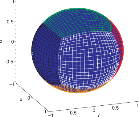
For example, what to do at the vertices of three patches meeting in the cubed-sphere case discussed later in this paper? As we will see, there we have three meshes with coordinates (at a constant radius) (a1,b1)superscript๐‘Ž1superscript๐‘1(a^{1},b^{1}), (a2,b2)superscript๐‘Ž2superscript๐‘2(a^{2},b^{2}), and (a3,b3)superscript๐‘Ž3superscript๐‘3(a^{3},b^{3}) arranged in a clockwise distribution according to the indices, and intersecting at a point. In that case, the contribution to the energy (without the penalty terms added to the evolution equations) is proportional to

(u0โ€‹N1,(Aa1+Ab1)โ€‹u0โ€‹N1)+(u002,(Aa2+Ab2)โ€‹u002)+(u0โ€‹N3,(Aa3+Ab3)โ€‹u0โ€‹N3)subscriptsuperscript๐‘ข10๐‘superscript๐ดsuperscript๐‘Ž1superscript๐ดsuperscript๐‘1subscriptsuperscript๐‘ข10๐‘subscriptsuperscript๐‘ข200superscript๐ดsuperscript๐‘Ž2superscript๐ดsuperscript๐‘2subscriptsuperscript๐‘ข200subscriptsuperscript๐‘ข30๐‘superscript๐ดsuperscript๐‘Ž3superscript๐ดsuperscript๐‘3subscriptsuperscript๐‘ข30๐‘(u^{1}_{0N},(A^{a^{1}}+A^{b^{1}})u^{1}_{0N})+(u^{2}_{00},(A^{a^{2}}+A^{b^{2}})u^{2}_{00})+(u^{3}_{0N},(A^{a^{3}}+A^{b^{3}})u^{3}_{0N})

Since the interfaces are aligned to the grids we know that the normals coincide on both sides, therefore we have:

Aa1=Aa3Ab1=Ab2Ab3=Aa2formulae-sequencesuperscript๐ดsuperscript๐‘Ž1superscript๐ดsuperscript๐‘Ž3formulae-sequencesuperscript๐ดsuperscript๐‘1superscript๐ดsuperscript๐‘2superscript๐ดsuperscript๐‘3superscript๐ดsuperscript๐‘Ž2A^{a^{1}}=A^{a^{3}}\;\;\;\;A^{b^{1}}=A^{b^{2}}\;\;\;\;A^{b^{3}}=A^{a^{2}}

So we include penalty terms on each side, including the end-points of the grids in each direction, (which constitute vertices and edges). Note that the characteristic modes at these points are computed with the normal with respect to the side that contains this direction. Consequently, points at edges/vertices of a (topologically) cubical grid will have two/three penalty terms.

III High order difference operators with diagonal norms

In this section we analyze some aspects of Strandโ€™s 111d difference operators satisfying SBP with respect to diagonal metrics, when used in conjuction with the penalty technique to construct high order schemes for handling domains with interfaces.

In particular, we discuss operators with accuracy of order two, four, six and eight at interior points. The requirement that these operators satisfy the SBP property with respect to diagonal norms implies that their respective accuracy order at and close to boundaries is one, two, three and four, respectively. We will therefore refer to these operators as D2โˆ’1,D4โˆ’2,D6โˆ’3subscript๐ท21subscript๐ท42subscript๐ท63D_{2-1},D_{4-2},D_{6-3}, and D8โˆ’4subscript๐ท84D_{8-4}. Some of these operators are not unique, as the accuracy order and SBP requirements still leave in some cases additional freedom in their construction. Indeed, while the first two operators (D2โˆ’1,D4โˆ’2subscript๐ท21subscript๐ท42D_{2-1},D_{4-2}) are unique, the D6โˆ’3subscript๐ท63D_{6-3} one comprises a mono-parametric family, and D8โˆ’4subscript๐ท84D_{8-4} a three-parametric one. This freedom can be exploited for several purposes. For instance, to minimize the operatorโ€™s bandwidth or its spectral radius. While the former produces operators which are more compact, the latter can have a significant impact on the CFL limit when dealing with evolution equations. Indeed, for the D8โˆ’4subscript๐ท84D_{8-4} case, minimizing its bandwidth leads to a considerably larger spectral radius (though this does not happen in the D6โˆ’3subscript๐ท63D_{6-3} case) which, in turns, requires one to employ a rather small CFL factor for the fully discrete scheme to be stable.

To analyze this in each case, we numerically solve and discuss the eigenvalues of the amplification matrix of the advection equation with speed one, ut=uโ€ฒsubscript๐‘ข๐‘กsuperscript๐‘ขโ€ฒu_{t}=u^{\prime}, under periodic boundary conditions. The periodicity is imposed through an interface with penalty terms and hence the scheme does depend on the penalty parameter ฮด๐›ฟ\delta and so will the discrete eigenvalues obtained. As discussed in Section II, in the case in which ฮด=โˆ’1/2๐›ฟ12\delta=-1/2, SBP holds across the interface, and the energy for this model is strictly conserved. In other words, the amplification matrix is anti-symmetric and the eigenvalues are purely imaginary (see Section II). On the other hand, if ฮด>โˆ’1/2๐›ฟ12\delta>-1/2 there is a negative definite interface term left after SBP, and a negative real component in the eigenvalues must appear in the spectrum of the amplification matrix (see Section II).

We additionally discuss the global convergence factor for these operators, and recall a feature associated with the mode with highest possible group speed at a given number of gridpoints. Namely, that it travels in the โ€œwrongโ€ direction, and that the absolute value of its speed increases considerably with the order of the operator.

Appendix A lists, for completeness, some typos in Ref. strand in some of the coefficients for these high order operators.

III.1 Spectrum

In the following we discuss the range of discrete eigenvalues obtained for the different derivative operators and their dependence on ฮด๐›ฟ\delta. We pay particular attention on the impact different values of ฮด๐›ฟ\delta and the chosen derivative operator have on the CFL limit.

III.1.1 Second order in the interior, first order at boundaries (D2โˆ’1subscript๐ท21D_{2-1} scheme)

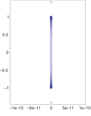
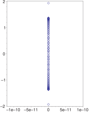
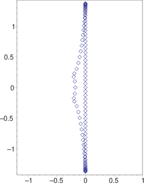
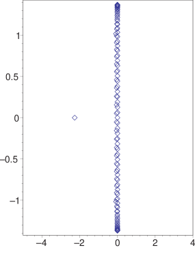
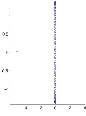
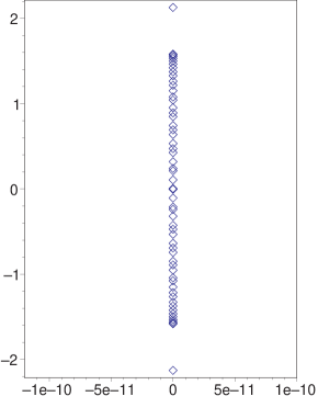
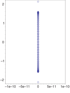
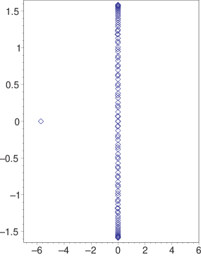
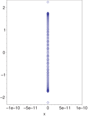
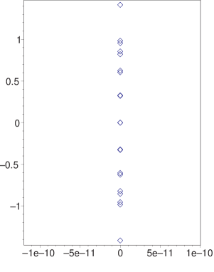
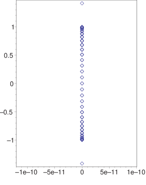
Figure 2 shows the eigenvalues obtained using 20,60,100206010020,60,100 gridpoints and penalty term ฮด=โˆ’1/2๐›ฟ12\delta=-1/2 (that is, the purely imaginary spectrum case, see Section II) for the D2โˆ’1subscript๐ท21D_{2-1} case. The maximum and minimum values are, approximately, ยฑ1.414plus-or-minus1.414\pm 1.414, and they seem to be related to the operator near the boundary, as their absolute value does not seem to increase with the number of points (instead, the region between the maximum and minimum is filled out). As discussed below, in the higher order cases the maximum eigenvalues also seem to be related to the operator near the boundary.
Refer to caption
Refer to caption
Refer to caption
Figure 2: Numerically obtained eigenvalues (in the complex plane) corresponding to the D2โˆ’1subscript๐ท21D_{2-1} operator for ฮด=โˆ’1/2๐›ฟ12\delta=-1/2 (purely imaginary case). From left to right the plots illustrate the results obtained with a grid containing 20,60,100206010020,60,100 points respectively. It is clear from the figures that these correspond, indeed, to a purely imaginary case.

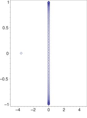
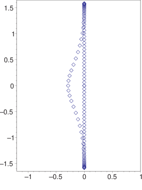
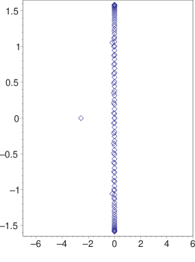
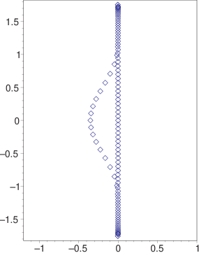
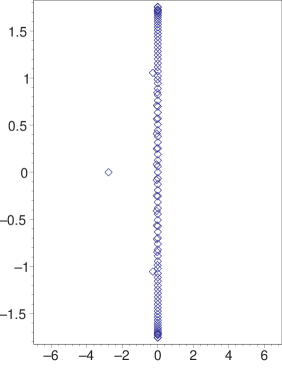
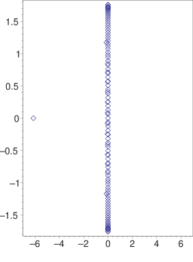
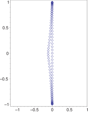
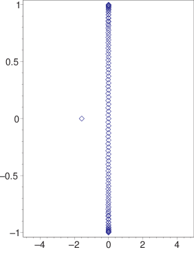
Figure 3, in turn, shows the eigenvalues computed with 100100100 points and ฮด=0,1/10,1/2๐›ฟ011012\delta=0,1/10,1/2. A negative real part appears, as it should (based on the energy calculation), and the maximum in the imaginary axis slightly decreases (to approximately 0.9990.9990.999, not varying much among these three values). However, the maximum absolute value in the negative real axis grows quite fast with ฮด๐›ฟ\delta. For example, for ฮด=1/10๐›ฟ110\delta=1/10 such maximum already dominates over the maximum in the imaginary axis. The higher order operators analyzed below behave similarly.
Refer to caption
Refer to caption
Refer to caption
Figure 3: Eigenvalues corresponding to the D2โˆ’1subscript๐ท21D_{2-1} operator, obtained with a grid containing 100100100 points. From left to right the plots illustrate the behavior for ฮด=0,1/10,1/2๐›ฟ011012\delta=0,1/10,1/2 respectively. As ฮด๐›ฟ\delta becomes larger, a larger (in magnitude) negative eigenvalue on the real axis is observed (notice the left-most diamond at yโ‰ƒโˆ’1.6,โˆ’3.5similar-to-or-equals๐‘ฆ1.63.5y\simeq-1.6,-3.5 on the middle and right plots, respectively).

III.1.2 Fourth order in the interior, second order at and close to boundaries (D4โˆ’2subscript๐ท42D_{4-2} scheme)

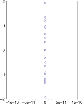
Figure 4 shows the equivalent of Figure 2, but now for the D4โˆ’2subscript๐ท42D_{4-2} case. The maximum is slightly larger than the corresponding one for the D2โˆ’1subscript๐ท21D_{2-1} case: approximately 1.9361.9361.936.

Refer to caption
Refer to caption
Refer to caption
Figure 4: Numerically obtained eigenvalues corresponding to the D4โˆ’2subscript๐ท42D_{4-2} operator for ฮด=โˆ’1/2๐›ฟ12\delta=-1/2 (purely imaginary case). From left to right the plots illustrate the results obtained with a grid containing 20,60,100206010020,60,100 points respectively. It is clear from the figures that these correspond, as in Fig.2, to a purely imaginary case.

Figure 5, in turn, shows the equivalent of Figure 3 for the current case. As before, a negative real part appears and the maximum in the imaginary axis slightly decreases (in this case to roughly 1.3711.3711.371, not changing much among these three values of ฮด๐›ฟ\delta).

Refer to caption
Refer to caption
Refer to caption
Figure 5: Eigenvalues corresponding to the D4โˆ’2subscript๐ท42D_{4-2} operator, obtained with a grid containing 100100100 points. From left to right the plots illustrate the behavior for ฮด=0,1/10,1/2๐›ฟ011012\delta=0,1/10,1/2 respectively. As ฮด๐›ฟ\delta becomes larger, a larger (in magnitude) negative eigenvalue on the real axis is observed (notice the left-most diamond at yโ‰ƒโˆ’2.5,โˆ’5similar-to-or-equals๐‘ฆ2.55y\simeq-2.5,-5 on the middle and right plots, respectively).

III.1.3 Sixth order in the interior, third order at and close to boundaries, minimum bandwidth case (D6โˆ’3subscript๐ท63D_{6-3} scheme)

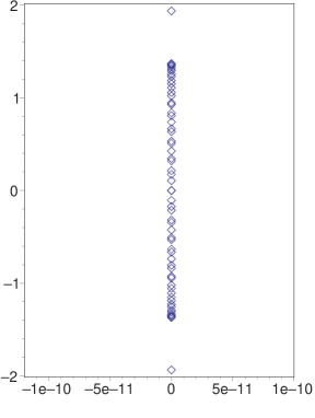
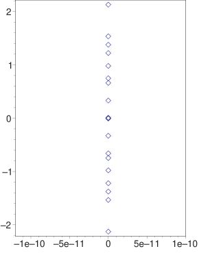
Figure 6 illustrates the equivalent of Figures (2,4) for the D6โˆ’3subscript๐ท63D_{6-3} case. The maximum is roughly 2.1292.1292.129, slightly larger than those of the previous two cases.
Refer to caption
Refer to caption
Refer to caption
Figure 6: Numerically obtained eigenvalues corresponding to the minimum bandwidth D6โˆ’3subscript๐ท63D_{6-3} operator for ฮด=โˆ’1/2๐›ฟ12\delta=-1/2 (purely imaginary case). From left to right the plots illustrate the results obtained with a grid containing 20,60,100206010020,60,100 points respectively. As in Figs.(2,4), these correspond to a purely imaginary case.

The behavior for larger values of ฮด๐›ฟ\delta is similar to that one found in the previous two cases, as seen in Figure 7. The maximum in the imaginary axis again decreases slightly compared to the ฮด=โˆ’1/2๐›ฟ12\delta=-1/2 case (to roughly 1.5851.5851.585) and does not change much among these three values of ฮด๐›ฟ\delta.

Refer to caption
Refer to caption
Refer to caption
Figure 7: Eigenvalues corresponding to the D6โˆ’3subscript๐ท63D_{6-3} operator obtained with a grid containing 100100100 points. From left to right the plots illustrate the behavior for ฮด=0,1/10,1/2๐›ฟ011012\delta=0,1/10,1/2 respectively. As ฮด๐›ฟ\delta becomes larger, a larger (in magnitude) negative eigenvalue on the real axis is observed (notice the left-most diamond at yโ‰ƒโˆ’2.5,โˆ’6similar-to-or-equals๐‘ฆ2.56y\simeq-2.5,-6 on the middle and right plots, respectively).

III.1.4 Eight order in the interior, fourth order at and close to boundaries (D8โˆ’4subscript๐ท84D_{8-4} scheme)

The D8โˆ’4subscript๐ท84D_{8-4} operator has three free parameters, denoted as x1,x2,x3subscript๐‘ฅ1subscript๐‘ฅ2subscript๐‘ฅ3x_{1},x_{2},x_{3} both in Ref.strand and here. As mentioned, these parameters can be freely chosen to satisfy a given criteria. For instance, they can be fixed so as to minimize the width of the derivative operator or yield as small a spectral radius as possible. As we discuss next, these options can yield operators with significantly different stability requirements as dictated by the CFL condition.

Minimum bandwidth operator. The minimum bandwidth case corresponds to the choice (see strand )

x1=17148374354560,x2=โˆ’102255130481920,x3=64456878709120.formulae-sequencesubscript๐‘ฅ117148374354560formulae-sequencesubscript๐‘ฅ2102255130481920subscript๐‘ฅ364456878709120x_{1}=\frac{1714837}{4354560},\;\;\;x_{2}=-\frac{1022551}{30481920},\;\;\;x_{3}=\frac{6445687}{8709120}. (27)

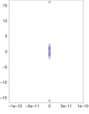
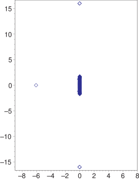
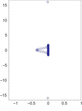
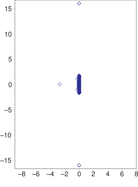
Figure 6 shows for this minimum D8โˆ’4subscript๐ท84D_{8-4} bandwidth case the eigenvalues for 20,60,100206010020,60,100 points, for ฮด=โˆ’1/2๐›ฟ12\delta=-1/2 (purely imaginary case). While for the previous operators we have seen that the maximum eigenvalue increases slightly with the order of the operator, in this case the increase is quite large: the maximum is roughly 16.0416.0416.04. This translates into a CFL limit for this operator being almost an order of magnitude smaller than the limits for the previous operators. Additionally, variation of ฮด๐›ฟ\delta does not significantly affect this behavior, as shown in Figure 9. That figure shows the eigenvalues computed with 100100100 points, and ฮด=0,1/10,1/2๐›ฟ011012\delta=0,1/10,1/2. The qualitative behavior when increasing ฮด๐›ฟ\delta is similar to that one of the previous cases. A negative real part appears in the spectrum, and the maximum in the imaginary axis slightly decreases, to roughly 16.0216.0216.02, not varying much among these three illustrative values of ฮด๐›ฟ\delta.

Refer to caption
Refer to caption
Refer to caption
Figure 8: Numerically obtained eigenvalues corresponding to the minimum bandwidth D8โˆ’4subscript๐ท84D_{8-4} operator for ฮด=โˆ’1/2๐›ฟ12\delta=-1/2 (purely imaginary case). From left to right the plots illustrate the results obtained with a grid containing 20,60,100206010020,60,100 points, respectively. Although purely imaginary, the maximum (absolute) value in the vertical axis is approximately 161616.

Such a large spectral radius for this operator motivates the search for another one, with a more convenient radius at the expense of not having the minimum possible bandwidth.
Refer to caption
Refer to caption
Refer to caption
Figure 9: Eigenvalues for the minimum bandwidth D8โˆ’4subscript๐ท84D_{8-4} operator with ฮด=0,1/10,1/2๐›ฟ011012\delta=0,1/10,1/2 (from left to right) and 100100100 points. Values of ฮด๐›ฟ\delta larger than โˆ’1/212-1/2 introduce a negative real part in the spectrum but they have little effect on the maximum absolute value, which remains at approximately 161616.

Optimized operator. We here construct an โ€œoptimized D8โˆ’4subscript๐ท84D_{8-4} operatorโ€ (which we shall use from here on in the D8โˆ’4subscript๐ท84D_{8-4} case) in the sense that it has a spectral radius considerably smaller than that one defined by Eq.(27). More precisely, through a numerical search in the three-parameter space we have found that the following values

x1=0.541,x2=โˆ’0.0675,x3=0.748,formulae-sequencesubscript๐‘ฅ10.541formulae-sequencesubscript๐‘ฅ20.0675subscript๐‘ฅ30.748x_{1}=0.541,\;\;\;x_{2}=-0.0675,\;\;\;x_{3}=0.748\,, (28)

yield an operator whose maximum absolute eigenvalue in the purely imaginary case (ฮด=โˆ’1/2๐›ฟ12\delta=-1/2) is

ฮปmโ€‹aโ€‹x=2.242.subscript๐œ†๐‘š๐‘Ž๐‘ฅ2.242\lambda_{max}=2.242\,. (29)

This maximum eigenvalue appears to be quite sensitive on these parameters. For example, truncating the above values to two significant digits,

x1=0.54,x2=โˆ’0.067,x3=0.75,formulae-sequencesubscript๐‘ฅ10.54formulae-sequencesubscript๐‘ฅ20.067subscript๐‘ฅ30.75x_{1}=0.54,\;\;\;x_{2}=-0.067,\;\;\;x_{3}=0.75\;,

gives ฮปmโ€‹aโ€‹x=2.698subscript๐œ†๐‘š๐‘Ž๐‘ฅ2.698\lambda_{max}=2.698 and truncating even more, to just one digit,

x1=0.5,x2=โˆ’0.07,x3=0.7,formulae-sequencesubscript๐‘ฅ10.5formulae-sequencesubscript๐‘ฅ20.07subscript๐‘ฅ30.7x_{1}=0.5,\;\;\;x_{2}=-0.07,\;\;\;x_{3}=0.7\;,

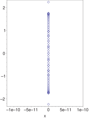
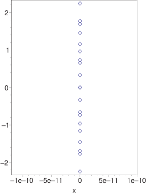
gives the large value ฮปmโ€‹aโ€‹x=71.76subscript๐œ†๐‘š๐‘Ž๐‘ฅ71.76\lambda_{max}=71.76. On the other hand, refining in the parameter search the values in Eq.(28) in one more digit did not change the maximum of Eq.(29) in its four digits here shown. The eigenvalues for ฮด=โˆ’1/2๐›ฟ12\delta=-1/2 for this optimized D8โˆ’4subscript๐ท84D_{8-4} operator, given by the parameters of Eq.(28), are shown in Figure 10, while
Refer to caption
Refer to caption
Refer to caption
Figure 10: Eigenvalues for the optimized D8โˆ’4subscript๐ท84D_{8-4} operator with ฮด=โˆ’1/2๐›ฟ12\delta=-1/2 (purely imaginary case), and 20,60,100206010020,60,100 points (from left to right). Clearly, this modified operator has a much smaller spectral radius, compared to the minimum bandwidth one.

Figure 11 shows them for ฮด=0,1/10,1/2๐›ฟ011012\delta=0,1/10,1/2 and 100100100 points. As before, a negative real component appears and the maximum in the imaginary axis decreases (to around 1.7541.7541.754).

Refer to caption
Refer to caption
Refer to caption
Figure 11: Eigenvalues for the optimized D8โˆ’4subscript๐ท84D_{8-4} operator, with 100100100 points and ฮด=0,1/10,1/2๐›ฟ011012\delta=0,1/10,1/2 (from left to right).

While completing this work we became aware of similar work by Svard, Mattson and Nordstrom smn , who construct an optimized operator with different parameters by minimizing the spectral radius of the derivative itself (rather than that of the amplification matrix of a toy problem with an interface, as in our case), obtaining x1=0.649,x2=โˆ’0.104,x3=0.755formulae-sequencesubscript๐‘ฅ10.649formulae-sequencesubscript๐‘ฅ20.104subscript๐‘ฅ30.755x_{1}=0.649,x_{2}=-0.104,x_{3}=0.755. When using these parameters in our toy problem with an interface, the resulting spectral radius (for twenty gridpoints) is ฮปmโ€‹aโ€‹x=2.241259subscript๐œ†๐‘š๐‘Ž๐‘ฅ2.241259\lambda_{max}=2.241259, while for the parameters we chose [cf. Eq.(28)] is ฮปmโ€‹aโ€‹x=2.241612subscript๐œ†๐‘š๐‘Ž๐‘ฅ2.241612\lambda_{max}=2.241612 pdiener .

III.2 Global convergence rate

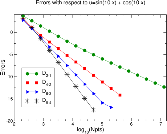
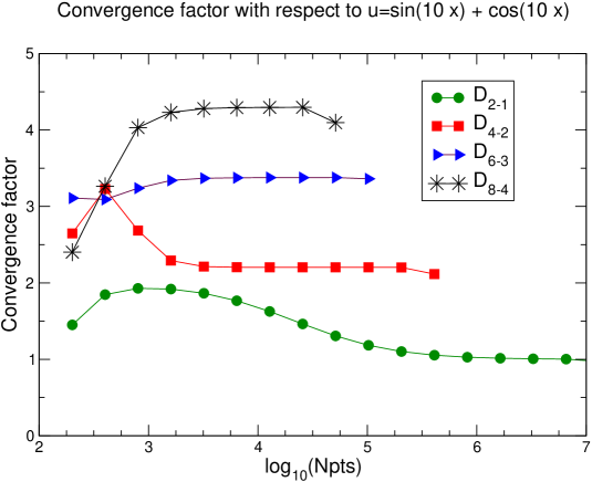
In general, the global (say, in an L2subscript๐ฟ2L_{2} norm) convergence factor for these operators will be dominated by the lower order at and close to boundaries. However, it is sometimes found that roundoff values for the error in such a global norm are reached before this happens, and the convergence factor is different from the one expected from the boundary terms. The precise value is found to actually depend on the function being differentiated and whether one reaches round-off level. To illustrate the expected behavior in a generic case, we consider the function sinโก(10โ€‹x)+cosโก(10โ€‹x)10๐‘ฅ10๐‘ฅ\sin(10x)+\cos(10x) in the domain xโˆˆ[0,2โ€‹ฯ€]๐‘ฅ02๐œ‹x\in[0,2\pi]. Figure 12 shows the error (with respect to the exact solution) when computing the discrete derivative versus the number of gridpoints, for the difference operators D2โˆ’1,D4โˆ’2,D6โˆ’3subscript๐ท21subscript๐ท42subscript๐ท63D_{2-1},D_{4-2},D_{6-3}, and D8โˆ’4subscript๐ท84D_{8-4}. The errors in the L2subscript๐ฟ2L_{2} norm are shown until roundoff values are reached (further increasing the number of gridpoints causes the error to grow with the number of points involved). Figure 13, in turn, shows the obtained convergence factors.
Refer to caption
Figure 12: L2subscript๐ฟ2L_{2} norms of the errors obtained when taking the discrete derivative of sinโก(10โ€‹x)+cosโก(10โ€‹x)10๐‘ฅ10๐‘ฅ\sin(10x)+\cos(10x) and comparing it with the analytical answer, using D2โˆ’1,D4โˆ’2,D6โˆ’3,D8โˆ’4subscript๐ท21subscript๐ท42subscript๐ท63subscript๐ท84D_{2-1},D_{4-2},D_{6-3},D_{8-4} operators, versus the number of gridpoints.
Refer to caption
Figure 13: Convergence factors for the curves of Figure 12. As in this case, the convergence in general will be dictated by the lower order the derivative operators have at and close to the boundaries. Note that the lines corresponding to the different operators terminate at sequentially fewer points. This is due to the corresponding errors reaching round-off levels, after which the convergence factor calculation ceases to have a sensible meaning.

III.3 Group Speed

We now turn our attention to the group speed that different discrete modes have when the above considered operators are used. To simplify the discussion, we actually restrict ourselves to the periodic case, which lends itself for a clean analytical calculation. In this case the operators of order two, four, six and eight satisfying SBP are the standard, centered ones (D0,D+,Dโˆ’subscript๐ท0subscript๐ทsubscript๐ทD_{0},D_{+},D_{-} denote the standard centered second order, and forward and backward first order operators, respectively):

D(2)superscript๐ท2\displaystyle D^{(2)} =\displaystyle= D0subscript๐ท0\displaystyle D_{0} (30)
D(4)superscript๐ท4\displaystyle D^{(4)} =\displaystyle= D0โ€‹(Iโˆ’h2/6โ€‹D+โ€‹Dโˆ’)subscript๐ท0๐ผsuperscriptโ„Ž26subscript๐ทsubscript๐ท\displaystyle D_{0}(I-h^{2}/6D_{+}D_{-}) (31)
D(6)superscript๐ท6\displaystyle D^{(6)} =\displaystyle= D0โ€‹(Iโˆ’h2/6โ€‹D+โ€‹Dโˆ’+h4/30โ€‹D+2โ€‹Dโˆ’2)subscript๐ท0๐ผsuperscriptโ„Ž26subscript๐ทsubscript๐ทsuperscriptโ„Ž430subscriptsuperscript๐ท2subscriptsuperscript๐ท2\displaystyle D_{0}(I-h^{2}/6D_{+}D_{-}+h^{4}/30D^{2}_{+}D^{2}_{-}) (32)
D(8)superscript๐ท8\displaystyle D^{(8)} =\displaystyle= D0โ€‹(Iโˆ’h2/6โ€‹D+โ€‹Dโˆ’+h4/30โ€‹D+2โ€‹Dโˆ’2โˆ’h6/140โ€‹D+3โ€‹Dโˆ’3)subscript๐ท0๐ผsuperscriptโ„Ž26subscript๐ทsubscript๐ทsuperscriptโ„Ž430subscriptsuperscript๐ท2subscriptsuperscript๐ท2superscriptโ„Ž6140subscriptsuperscript๐ท3subscriptsuperscript๐ท3\displaystyle D_{0}(I-h^{2}/6D_{+}D_{-}+h^{4}/30D^{2}_{+}D^{2}_{-}-h^{6}/140D^{3}_{+}D^{3}_{-}) (33)

In discrete Fourier space, the eigenvalues for these operators are, respectively,

ฮป2subscript๐œ†2\displaystyle\lambda_{2} =\displaystyle= sinโก(ฮถ)/ฮถ,๐œ๐œ\displaystyle\sin(\zeta)/\zeta\,, (35)
ฮป4subscript๐œ†4\displaystyle\lambda_{4} =\displaystyle= sinโก(ฮถ)/ฮถโ€‹(1+2โ€‹sinโก(ฮถ/2)/3),๐œ๐œ12๐œ23\displaystyle\sin(\zeta)/\zeta(1+2\sin(\zeta/2)/3)\,, (36)
ฮป6subscript๐œ†6\displaystyle\lambda_{6} =\displaystyle= sinโก(ฮถ)/ฮถโ€‹(1+2โ€‹sinโก(ฮถ/2)/3+8โ€‹sin4โก(ฮถ/2)/15),๐œ๐œ12๐œ238superscript4๐œ215\displaystyle\sin(\zeta)/\zeta(1+2\sin(\zeta/2)/3+8\sin^{4}(\zeta/2)/15)\,, (37)
ฮป8subscript๐œ†8\displaystyle\lambda_{8} =\displaystyle= sinโก(ฮถ)/ฮถโ€‹(1+2โ€‹sinโก(ฮถ/2)/3+8โ€‹sin4โก(ฮถ/2)/15+64โ€‹sin6โก(ฮถ/2)/140).๐œ๐œ12๐œ238superscript4๐œ21564superscript6๐œ2140\displaystyle\sin(\zeta)/\zeta(1+2\sin(\zeta/2)/3+8\sin^{4}(\zeta/2)/15+64\sin^{6}(\zeta/2)/140)\,. (38)

where ฮถ=ฯ‰โ€‹h๐œ๐œ”โ„Ž\zeta=\omega h, and ฯ‰๐œ”\omega is the associated wave number.

The highest possible frequency is ฯ‰=N/2๐œ”๐‘2\omega=N/2 (with N๐‘N the number of gridpoints). For that frequency, ฮถ=ฯ€๐œ๐œ‹\zeta=\pi and the above eigenvalues are all zero. Therefore the mode with highest possible frequency for a given number of points does not propagate. Furthermore, if one examines the group speed,

vg=dโ€‹(ฮปโ€‹ฯ‰)dโ€‹ฯ‰,subscript๐‘ฃ๐‘”๐‘‘๐œ†๐œ”๐‘‘๐œ”v_{g}=\frac{d(\lambda\omega)}{d\omega}\,, (39)

one finds that at ฮถ=ฯ€๐œ๐œ‹\zeta=\pi this speed is

vg2superscriptsubscript๐‘ฃ๐‘”2\displaystyle v_{g}^{2} =\displaystyle= โˆ’1,1\displaystyle-1\,, (40)
vg4superscriptsubscript๐‘ฃ๐‘”4\displaystyle v_{g}^{4} =\displaystyle= โˆ’5/3โ‰ˆโˆ’1.6,531.6\displaystyle-5/3\approx-1.6\,, (41)
vg6superscriptsubscript๐‘ฃ๐‘”6\displaystyle v_{g}^{6} =\displaystyle= โˆ’33/15โ‰ˆโˆ’2.2,33152.2\displaystyle-33/15\approx-2.2\,, (42)
vg8superscriptsubscript๐‘ฃ๐‘”8\displaystyle v_{g}^{8} =\displaystyle= โˆ’341/135โ‰ˆโˆ’2.6.3411352.6\displaystyle-341/135\approx-2.6\,. (43)

Thus, for higher (than two) order operators the velocity of this mode is higher than the continuum one (which is 111). But, more importantly, in all cases the speed has the opposite sign. Of course, this effect goes away with resolution, since the highest possible frequency moves to larger values as resolution is increased. But, still, is an effect to be taken into account. For instance, if noise is produced at an interface, it propagates backwards, and with higher speed. Even though this effect is typically very small, it might be noticeable in highly accurate simulations, or in simulations in which the solution itself decays to very small values (see Section IV.3.2). This could also be a source of difficulties in the presence of black holes โ€“or for this matter any system where some propagation speed changes signโ€“ since the event horizon traps these high frequency modes in a very narrow region and then releases them as low frequency ones. We have observed this in some highly resolved one dimensional simulations, and explains an observed convergence drop which goes away when numerical dissipation is turned on.

IV Tests

In this section we illustrate the behavior of the aforementioned penalty technique, together with the choice of different derivative operators. We present tests in one, two and three dimensions. In particular, we implement the linearized Einstein equations (off a โ€˜gauge-waveโ€™ spacetime weakhyp ; apples ) and propagation of scalar fields in black hole backgrounds. The former is cast in a way which yields a one-dimensional symmetric hyperbolic system with coefficients depending both in space and time while the latter provides an hyperbolic system of equations with space varying coefficients and sets a conforming grid for spherical black hole excision.

Throughout this paper we employ a fourth order accurate Rungeโ€“Kutta time integrator. In a number of tests aimed at examining the behavior of high order operators we adopt a sufficiently small time step ฮ”โ€‹tฮ”๐‘ก\Delta t so that the time integrator does not play a role. Thus, we either choose a suitably small CFL factor or we scale the time step quadratically with the gridspacing hโ„Žh.

IV.1 One dimensional simulations: linearizations around a gauge wave

As a first test we evolve Einsteinโ€™s equations in one dimension, linearized around a background given by

dโ€‹s2=eAโ€‹sinโก(ฯ€โ€‹(xโˆ’t))โ€‹(โˆ’dโ€‹t2+dโ€‹x2)+dโ€‹y2+dโ€‹z2.๐‘‘superscript๐‘ 2superscript๐‘’๐ด๐œ‹๐‘ฅ๐‘ก๐‘‘superscript๐‘ก2๐‘‘superscript๐‘ฅ2๐‘‘superscript๐‘ฆ2๐‘‘superscript๐‘ง2ds^{2}=e^{A\sin(\pi(x-t))}(-{dt}^{2}+{dx}^{2})+{dy}^{2}+{dz}^{2}. (44)

This background describes flat spacetime with a sinusoidal coordinate dependence, of amplitude A๐ดA, along the x๐‘ฅx direction. One of the interesting features of this testbed is that while a linear problem, the coefficients in the equations to solve are not only space but also time dependent.

The non-trivial variables for this metric are

g^xโ€‹xsubscript^๐‘”๐‘ฅ๐‘ฅ\displaystyle\hat{g}_{xx} =\displaystyle= eAโ€‹sinโก(ฯ€โ€‹(xโˆ’t)),superscript๐‘’๐ด๐œ‹๐‘ฅ๐‘ก\displaystyle e^{A\sin(\pi(x-t))}\,, (45)
K^xโ€‹xsubscript^๐พ๐‘ฅ๐‘ฅ\displaystyle\hat{K}_{xx} =\displaystyle= A2โ€‹ฯ€โ€‹cosโก(ฯ€โ€‹(xโˆ’t))โ€‹eA/2โ€‹sinโก(ฯ€โ€‹(xโˆ’t)),๐ด2๐œ‹๐œ‹๐‘ฅ๐‘กsuperscript๐‘’๐ด2๐œ‹๐‘ฅ๐‘ก\displaystyle\frac{A}{2}\pi\cos\left(\pi\left(x-t\right)\right)e^{A/2\sin\left(\pi\left(x-t\right)\right)}\;, (46)
ฮฑ^^๐›ผ\displaystyle\hat{\alpha} =\displaystyle= eA/2โ€‹sinโก(ฯ€โ€‹(xโˆ’t)),superscript๐‘’๐ด2๐œ‹๐‘ฅ๐‘ก\displaystyle e^{A/2\sin\left(\pi\left(x-t\right)\right)}\,, (47)
ฮฒ^isuperscript^๐›ฝ๐‘–\displaystyle\hat{\beta}^{i} =\displaystyle= 0.0\displaystyle 0\,. (48)

We evolve the linearized Einstein equations using the symmetric hyperbolic formulation presented in Ref.ย sarbach-tiglio with a dynamical lapse given by the homogeneous time-harmonic condition (defined by requiring โ–กโ€‹t=0โ–ก๐‘ก0\square t=0). The formulation is cast in first order form by introducing the variables ๐’œx:=โˆ‚xฮฑ/ฮฑassignsubscript๐’œ๐‘ฅsubscript๐‘ฅ๐›ผ๐›ผ{\cal A}_{x}:=\partial_{x}\alpha/\alpha and dxโ€‹xโ€‹x:=โˆ‚xgxโ€‹xassignsubscript๐‘‘๐‘ฅ๐‘ฅ๐‘ฅsubscript๐‘ฅsubscript๐‘”๐‘ฅ๐‘ฅd_{xxx}:=\partial_{x}g_{xx}. The equations determining the dynamics of the (first order) perturbations, which we assume to depend solely on (t,x)๐‘ก๐‘ฅ(t,x), are obtained by considering linear deviations of a background metric given by Eq.ย (44). That is, we consider

gxโ€‹xsubscript๐‘”๐‘ฅ๐‘ฅ\displaystyle g_{xx} =\displaystyle= g^xโ€‹x+ฮดโ€‹gxโ€‹x,subscript^๐‘”๐‘ฅ๐‘ฅ๐›ฟsubscript๐‘”๐‘ฅ๐‘ฅ\displaystyle\hat{g}_{xx}+\delta g_{xx},
Kxโ€‹xsubscript๐พ๐‘ฅ๐‘ฅ\displaystyle K_{xx} =\displaystyle= K^xโ€‹x+ฮดโ€‹Kxโ€‹x,subscript^๐พ๐‘ฅ๐‘ฅ๐›ฟsubscript๐พ๐‘ฅ๐‘ฅ\displaystyle\hat{K}_{xx}+\delta K_{xx},
dxโ€‹xโ€‹xsubscript๐‘‘๐‘ฅ๐‘ฅ๐‘ฅ\displaystyle d_{xxx} =\displaystyle= d^xโ€‹xโ€‹x+ฮดโ€‹dxโ€‹xโ€‹x,subscript^๐‘‘๐‘ฅ๐‘ฅ๐‘ฅ๐›ฟsubscript๐‘‘๐‘ฅ๐‘ฅ๐‘ฅ\displaystyle\hat{d}_{xxx}+\delta d_{xxx},
ฮฑ๐›ผ\displaystyle\alpha =\displaystyle= ฮฑ^+ฮดโ€‹ฮฑ,^๐›ผ๐›ฟ๐›ผ\displaystyle\hat{\alpha}+\delta\alpha,
๐’œxsubscript๐’œ๐‘ฅ\displaystyle{\cal A}_{x} =\displaystyle= ๐’œ^x+ฮดโ€‹๐’œx;subscript^๐’œ๐‘ฅ๐›ฟsubscript๐’œ๐‘ฅ\displaystyle\hat{\cal A}_{x}+\delta{\cal A}_{x}\,;

replace these expressions in Einsteinโ€™s equations and retain only first order terms. The resulting equations are (henceforth dropping the ฮด๐›ฟ\delta notation)

ฮฑห™ห™๐›ผ\displaystyle\dot{\alpha} =\displaystyle= โˆ’Aโ€‹ฯ€โ€‹cosโก(ฯ•)โ€‹ฮฑโˆ’Kxโ€‹x+Aโ€‹ฯ€2โ€‹ฮฑ^โ€‹cosโก(ฯ•)โ€‹gxโ€‹x,๐ด๐œ‹italic-ฯ•๐›ผsubscript๐พ๐‘ฅ๐‘ฅ๐ด๐œ‹2^๐›ผitalic-ฯ•subscript๐‘”๐‘ฅ๐‘ฅ\displaystyle-A\pi\cos(\phi)\alpha-K_{xx}+\frac{A\pi}{2\hat{\alpha}}\cos(\phi)g_{xx}\,, (49)
๐’œห™xsubscriptห™๐’œ๐‘ฅ\displaystyle\dot{\cal A}_{x} =\displaystyle= โˆ’1ฮฑ^โ€‹โˆ‚xKxโ€‹x+Aโ€‹ฯ€2โ€‹ฮฑ^โ€‹cosโก(ฯ•)โ€‹Kxโ€‹x,1^๐›ผsubscript๐‘ฅsubscript๐พ๐‘ฅ๐‘ฅ๐ด๐œ‹2^๐›ผitalic-ฯ•subscript๐พ๐‘ฅ๐‘ฅ\displaystyle-\frac{1}{\hat{\alpha}}\partial_{x}K_{xx}+\frac{A\pi}{2\hat{\alpha}}\cos(\phi)K_{xx}\,, (50)
โˆ’Aโ€‹ฯ€22โ€‹ฮฑ^2(Acos(ฯ•)2+sin(ฯ•))gxโ€‹x\displaystyle-\frac{A\pi^{2}}{2\hat{\alpha}^{2}}\left(A\cos(\phi)^{2}+\sin(\phi)\right)g_{xx}
+Aโ€‹ฯ€2โ€‹ฮฑ^2โ€‹cosโก(ฯ•)โ€‹dxโ€‹xโ€‹x๐ด๐œ‹2superscript^๐›ผ2italic-ฯ•subscript๐‘‘๐‘ฅ๐‘ฅ๐‘ฅ\displaystyle+\frac{A\pi}{2\hat{\alpha}^{2}}\cos(\phi)d_{xxx}
โˆ’Aโ€‹ฯ€2โ€‹cosโก(ฯ•)โ€‹๐’œx+Aโ€‹ฯ€22โ€‹ฮฑ^โ€‹sinโก(ฯ•)โ€‹ฮฑ,๐ด๐œ‹2italic-ฯ•subscript๐’œ๐‘ฅ๐ดsuperscript๐œ‹22^๐›ผitalic-ฯ•๐›ผ\displaystyle-\frac{A\pi}{2}\cos(\phi){\cal A}_{x}+\frac{A\pi^{2}}{2\hat{\alpha}}\sin(\phi)\alpha\,,
gห™xโ€‹xsubscriptห™๐‘”๐‘ฅ๐‘ฅ\displaystyle\dot{g}_{xx} =\displaystyle= โˆ’Aโ€‹ฮฑ^โ€‹ฯ€โ€‹cosโก(ฯ•)โ€‹ฮฑโˆ’2โ€‹ฮฑ^โ€‹Kxโ€‹x,๐ด^๐›ผ๐œ‹italic-ฯ•๐›ผ2^๐›ผsubscript๐พ๐‘ฅ๐‘ฅ\displaystyle-A\hat{\alpha}\pi\cos(\phi)\alpha-2\hat{\alpha}K_{xx}\,, (51)
Kห™xโ€‹xsubscriptห™๐พ๐‘ฅ๐‘ฅ\displaystyle\dot{K}_{xx} =\displaystyle= โˆ’ฮฑ^โ€‹โˆ‚x๐’œxโˆ’Aโ€‹ฮฑ^โ€‹ฯ€2โ€‹cosโก(ฯ•)โ€‹๐’œx^๐›ผsubscript๐‘ฅsubscript๐’œ๐‘ฅ๐ด^๐›ผ๐œ‹2italic-ฯ•subscript๐’œ๐‘ฅ\displaystyle-\hat{\alpha}\partial_{x}{\cal A}_{x}-\frac{A\hat{\alpha}\pi}{2}\cos(\phi){\cal A}_{x} (52)
โˆ’Aโ€‹ฯ€24(โˆ’2sin(ฯ•)+Acos(ฯ•)2)ฮฑ\displaystyle-\frac{A\pi^{2}}{4}\left(-2\sin(\phi)+A\cos(\phi)^{2}\right)\alpha
โˆ’Aโ€‹ฯ€โ€‹cosโก(ฯ•)โ€‹Kxโ€‹x๐ด๐œ‹italic-ฯ•subscript๐พ๐‘ฅ๐‘ฅ\displaystyle-A\pi\cos(\phi)K_{xx}
+Aโ€‹ฯ€4โ€‹ฮฑ^โ€‹cosโก(ฯ•)โ€‹dxโ€‹xโ€‹x,๐ด๐œ‹4^๐›ผitalic-ฯ•subscript๐‘‘๐‘ฅ๐‘ฅ๐‘ฅ\displaystyle+\frac{A\pi}{4\hat{\alpha}}\cos(\phi)d_{xxx}\,,
dห™xโ€‹xโ€‹xsubscriptห™๐‘‘๐‘ฅ๐‘ฅ๐‘ฅ\displaystyle\dot{d}_{xxx} =\displaystyle= Aฮฑ^ฯ€2(sin(ฯ•)โˆ’Acos(ฯ•)2)ฮฑ\displaystyle{A\hat{\alpha}\pi^{2}}\left(\sin(\phi)-A\cos(\phi)^{2}\right)\alpha (53)
โˆ’Aโ€‹ฮฑ^โ€‹ฯ€โ€‹cosโก(ฯ•)โ€‹Kxโ€‹xโˆ’Aโ€‹ฮฑ^2โ€‹ฯ€โ€‹cosโก(ฯ•)โ€‹๐’œx๐ด^๐›ผ๐œ‹italic-ฯ•subscript๐พ๐‘ฅ๐‘ฅ๐ดsuperscript^๐›ผ2๐œ‹italic-ฯ•subscript๐’œ๐‘ฅ\displaystyle-A\hat{\alpha}\pi\cos(\phi)K_{xx}-A\hat{\alpha}^{2}\pi\cos(\phi){\cal A}_{x}
โˆ’2โ€‹ฮฑ^โ€‹โˆ‚xKxโ€‹x,2^๐›ผsubscript๐‘ฅsubscript๐พ๐‘ฅ๐‘ฅ\displaystyle-2\hat{\alpha}\partial_{x}K_{xx}\,,

where we have defined ฯ•:=ฯ€โ€‹(xโˆ’t)assignitalic-ฯ•๐œ‹๐‘ฅ๐‘ก\phi:=\pi(x-t). This system is symmetric hyperbolic and the symmetrizer used to define the energy can be chosen so that the characteristic speeds which play a role in the energy estimate are 00 and ยฑ1plus-or-minus1\pm 1.

We consider here a periodic initial boundary value problem on the domain xโˆˆ[โˆ’1/2,3/2]๐‘ฅ1232x\in[-1/2,3/2], where periodic boundary conditions at x=โˆ’1/2,3/2๐‘ฅ1232x=-1/2,3/2 are implemented through an interface with penalty terms, as described in Section II.

The system must satisfy two non-trivial constraint equations, corresponding to the definition of the variables dxโ€‹xโ€‹xsubscript๐‘‘๐‘ฅ๐‘ฅ๐‘ฅd_{xxx} and ๐’œxsubscript๐’œ๐‘ฅ{\cal A}_{x} (the linearized physical constraints are automatically satisfied by the considered ansatz). When linearized, these constraints are

00\displaystyle 0 =\displaystyle= Cx=โˆ’โˆ‚xgxโ€‹x+dxโ€‹xโ€‹x,subscript๐ถ๐‘ฅsubscript๐‘ฅsubscript๐‘”๐‘ฅ๐‘ฅsubscript๐‘‘๐‘ฅ๐‘ฅ๐‘ฅ\displaystyle C_{x}=-\partial_{x}g_{xx}+d_{xxx}\;, (54)
00\displaystyle 0 =\displaystyle= C๐’œ=๐’œxโˆ’1ฮฑ^โ€‹(โˆ‚xฮฑโˆ’Aโ€‹ฯ€2โ€‹cosโก(ฯ•)โ€‹ฮฑ).subscript๐ถ๐’œsubscript๐’œ๐‘ฅ1^๐›ผsubscript๐‘ฅ๐›ผ๐ด๐œ‹2italic-ฯ•๐›ผ\displaystyle C_{\cal A}={\cal A}_{x}-\frac{1}{\hat{\alpha}}\left(\partial_{x}\alpha-\frac{A\pi}{2}\cos(\phi)\alpha\right). (55)

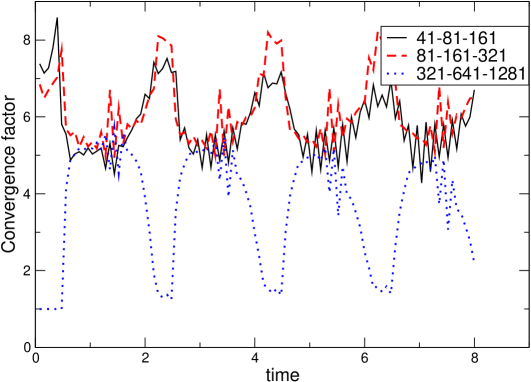
In the first series of simulations we adopt a CFL factor ฮป=10โˆ’3๐œ†superscript103\lambda=10^{-3}444We do not claim that this is the largest possible CFL factor for which the errors due to time integration are negligible compared to the spatial ones, though. Actually, as discussed later, in some cases one can use larger CFL factors. and consider relatively short evolutions corresponding to four crossing times. The D8โˆ’4subscript๐ท84D_{8-4} derivative is used, and dissipation is added through the dissipative operator constructed from โˆ’ฯƒโ€‹h7โ€‹D+4โ€‹Dโˆ’4๐œŽsuperscriptโ„Ž7superscriptsubscript๐ท4superscriptsubscript๐ท4-\sigma h^{7}D_{+}^{4}D_{-}^{4}, suitably modified at boundaries as explained in Appendix B so as to make it non-positive definite with respect to the appropriate scalar product. Thus, the use of this dissipative operator does decrease the order of the spatial discretization by one. The dissipation parameter used is ฯƒ=5ร—10โˆ’4๐œŽ5superscript104\sigma=5\times 10^{-4}. Figure 14 exemplifies the behavior observed in the convergence of the field Kxโ€‹xsubscript๐พ๐‘ฅ๐‘ฅK_{xx} (the other fields behave similarly). As time progresses the convergence order obtained oscillates in a way that is consistent with the accuracy obtained at interior and boundary points.
Refer to caption
Figure 14: Evolutions of 111d linearized Einsteinโ€™s equations in a periodic domain, with periodicity enforced through an interface with penalty terms. Shown is the convergence factor for Kxโ€‹xsubscript๐พ๐‘ฅ๐‘ฅK_{xx} when using the D8โˆ’4subscript๐ท84D_{8-4} derivative, CFL factor ฮป=10โˆ’3๐œ†superscript103\lambda=10^{-3}, and dissipation ฯƒ=5ร—10โˆ’4๐œŽ5superscript104\sigma=5\times 10^{-4}. While the convergence factors obtained with 414141 to 321321321 points oscillate between the expected order at the boundary and that one at the interior, the ones calculated with 321321321 to 128112811281 points are not meaningful when the pulse is located at interior points as round-off level is reached.

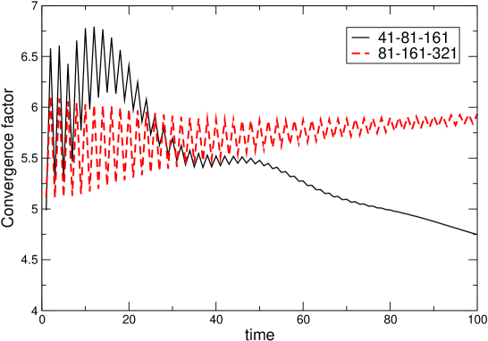
Next, we adopt as a starting value for the CFL factor defined at the coarsest grip to be ฮป=0.2๐œ†0.2\lambda=0.2 but in subsequent grids (refined by a factor of 222) we adopt ฮป=0.2/2n๐œ†0.2superscript2๐‘›\lambda=0.2/2^{n} with (n=1..3)๐‘›1..3(n=1..3). Figure 15 illustrates the behavior observed; again, as time progresses the convergence order obtained oscillates in between the order of accuracy of interior and boundary points, with the additional effect of accuracy loss due to the accumulation of error as time progresses.
Refer to caption
Figure 15: Same as previous figure, but with a decreasing CFL factor given by ฮป=0.2/2n๐œ†0.2superscript2๐‘›\lambda=0.2/2^{n} with (n=1..3)๐‘›1..3(n=1..3).

.

Finally, we compare the above results with those obtained in the โ€œtruly periodic caseโ€, ie. when periodicity is used explicitly to employ the same derivative operator at all points. We again consider cases where a sufficiently small CFL factor (=10โˆ’3absentsuperscript103=10^{-3}) is used or the time-step is scaled quadratically. Figures 16 illustrates the observed convergence rate for the field gxโ€‹xsubscript๐‘”๐‘ฅ๐‘ฅg_{xx}. As above, dissipation is added through a seventh order dissipative operator (but now with no modification at boundaries needed) with same dissipative parameter: ฯƒ=5ร—10โˆ’4๐œŽ5superscript104\sigma=5\times 10^{-4}. While the errors remain above round-off level the observed convergence rate is consistent with the expected one of seven, as the orders of the derivative and dissipative operators employed are eight and seven respectively. Certainly, dissipation of higher order could have been introduced by simply employing the KO style operator h9โ€‹(Dโˆ’โ€‹D+)5superscriptโ„Ž9superscriptsubscript๐ทsubscript๐ท5h^{9}(D_{-}D_{+})^{5}, but we have adopted this one to more directly compare with the case with interface boundaries. For the highest resolutions the errors reach round-off level and the obtained convergence factors yield non-sensible values.
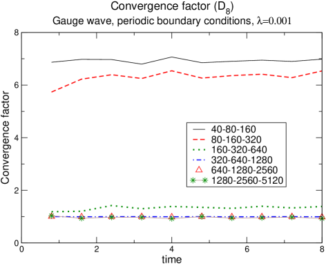
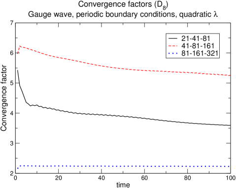
Refer to caption
Refer to caption
Figure 16: This figure shows evolutions similar to those of Figs.14, 15, with the only difference that periodicity is here enforced explicitly. The convergence factors for the metric component gxโ€‹xsubscript๐‘”๐‘ฅ๐‘ฅg_{xx} are shown.

.

As an illustration of what is observed with other derivatives, we briefly discuss some simulations using the D6โˆ’3subscript๐ท63D_{6-3} operator and a fixed CFL factor (given, as before, by ฮป=10โˆ’3๐œ†superscript103\lambda=10^{-3}). Analogously as to was done above, dissipation is here added by extending โ€“as discussed in Appendix Bโ€“ the operator ฯƒโ€‹h6โ€‹Dโˆ’3โ€‹D+3๐œŽsuperscriptโ„Ž6superscriptsubscript๐ท3superscriptsubscript๐ท3\sigma h^{6}D_{-}^{3}D_{+}^{3} at and near boundaries in order to make it non-positive definite with respect to the appropriate scalar product; a dissipation parameter ฯƒ=10โˆ’3๐œŽsuperscript103\sigma=10^{-3} is used. The observed results are illustrated in Figure 17, which shows the self-convergence factor for Kxโ€‹xsubscript๐พ๐‘ฅ๐‘ฅK_{xx}. As before, it oscillates between the order of the scheme in the interior and that one at boundary points.
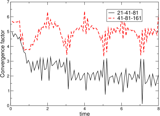
Refer to caption
Figure 17: Similar to Fig. 14, but using the D6โˆ’3subscript๐ท63D_{6-3} derivative. The convergence factor for Kxโ€‹xsubscript๐พ๐‘ฅ๐‘ฅK_{xx} is shown.

Summarizing, the results presented indicate that, in the case where boundaries are present, the worst case scenario โ€“as far as the expected convergence rate relatesโ€“ is determined by the accuracy order at and close to boundary points.

Two and three-dimensional simulations. Problem set-up

In this section we solve the wave equation for a scalar field ฯ•italic-ฯ•\phi propagating on a fixed background,

โˆ‡aโˆ‡aโกฯ•=0,superscriptโˆ‡๐‘Žsubscriptโˆ‡๐‘Žitalic-ฯ•0\nabla^{a}\nabla_{a}\phi=0\,,

where โˆ‡โˆ‡\nabla is the covariant derivative associated with the metric of the background. We will consider two backgrounds: a 222d one consisting of the unit sphere with its standard metric and a 333d one consisting of a rotating Kerr black hole background.

We start by describing in more detail the equations solved and the multiple coordinate system used, and then present the actual results of the simulations.

A strictly stable scheme for the wave equation in a time-independent, curved spacetime

The wave equation in a time-independent background can be written, using any coordinates in which the metric is manifestly time independent as,

ฯ•ห™ห™italic-ฯ•\displaystyle\dot{\phi} =\displaystyle= ฮฑโ€‹ฮ ๐›ผฮ \displaystyle\alpha\Pi (56)
ฮ ห™ห™ฮ \displaystyle\dot{\Pi} =\displaystyle= ฮฒiโ€‹ฮฑโˆ’1โ€‹Diโ€‹(ฮฑโ€‹ฮ )+hโˆ’1/2โ€‹Diโ€‹(h1/2โ€‹ฮฒiโ€‹ฮ +ฮฑโ€‹h1/2โ€‹Hiโ€‹jโ€‹dj)superscript๐›ฝ๐‘–superscript๐›ผ1subscript๐ท๐‘–๐›ผฮ superscriptโ„Ž12subscript๐ท๐‘–superscriptโ„Ž12superscript๐›ฝ๐‘–ฮ ๐›ผsuperscriptโ„Ž12superscript๐ป๐‘–๐‘—subscript๐‘‘๐‘—\displaystyle\beta^{i}\alpha^{-1}D_{i}(\alpha\Pi)+h^{-1/2}D_{i}(h^{1/2}\beta^{i}\Pi+\alpha h^{1/2}H^{ij}d_{j}) (57)
dห™isubscriptห™๐‘‘๐‘–\displaystyle\dot{d}_{i} =\displaystyle= Diโ€‹(ฮฑโ€‹ฯ€)subscript๐ท๐‘–๐›ผ๐œ‹\displaystyle D_{i}(\alpha\pi) (58)

where Hiโ€‹j:=hiโ€‹jโˆ’ฮฑโˆ’2โ€‹ฮฒiโ€‹ฮฒjassignsuperscript๐ป๐‘–๐‘—superscriptโ„Ž๐‘–๐‘—superscript๐›ผ2superscript๐›ฝ๐‘–superscript๐›ฝ๐‘—H^{ij}:=h^{ij}-\alpha^{-2}\beta^{i}\beta^{j}, hiโ€‹jsuperscriptโ„Ž๐‘–๐‘—h^{ij} is the inverse of the three-metric, h=detโ€‹(hiโ€‹j)โ„Ždetsubscriptโ„Ž๐‘–๐‘—h={\rm det}(h_{ij}), ฮฑ๐›ผ\alpha is the lapse and ฮฒisuperscript๐›ฝ๐‘–\beta^{i} the shift vector. The advantage of writing the equations in this way is that one can show that if D๐ทD is any difference operator satisfying SBP, this form of the equations guarantees that the semidiscrete version of the physical energy is a non-increasing function of time. When the killing field is timelike this means that there is a norm in which the solution is bounded for all times, thus suppressing artificial fast growing-modes without the need of artificial dissipation (see strict for details).

We now look at the characteristic variables and characteristic speeds with respect to a โ€œcoordinateโ€ observer. That is, the eigenfields and eigenvalues of the symbol Aiโ€‹nisuperscript๐ด๐‘–subscript๐‘›๐‘–A^{i}n_{i}, where Aisuperscript๐ด๐‘–A^{i} denotes the principal part of the evolution equations and nisubscript๐‘›๐‘–n_{i} the normal to the boundary 555If the boundary is aligned with the coordinates lines, as is indeed the case here, nisubscript๐‘›๐‘–n_{i} would be either (1,0,0)100(1,0,0), (0,1,0)010(0,1,0), or (0,0,1)001(0,0,1).. The characteristic variables with non-zero speeds

ฮปยฑ=(ยฑฮฑ+ฮฒkโ€‹n^k)โ€‹(hiโ€‹jโ€‹niโ€‹nj)1/2superscript๐œ†plus-or-minusplus-or-minus๐›ผsuperscript๐›ฝ๐‘˜subscript^๐‘›๐‘˜superscriptsuperscriptโ„Ž๐‘–๐‘—subscript๐‘›๐‘–subscript๐‘›๐‘—12\lambda^{\pm}=(\pm\alpha+\beta^{k}\hat{n}_{k})(h^{ij}n_{i}n_{j})^{1/2}

[where n^k=nkโ€‹(hiโ€‹jโ€‹niโ€‹nj)โˆ’1/2subscript^๐‘›๐‘˜subscript๐‘›๐‘˜superscriptsuperscriptโ„Ž๐‘–๐‘—subscript๐‘›๐‘–subscript๐‘›๐‘—12\hat{n}_{k}=n_{k}(h^{ij}n_{i}n_{j})^{-1/2}] are

vยฑ=ฮปยฑโ€‹ฮ +ฮฑโ€‹Hiโ€‹jโ€‹n^iโ€‹dj;superscript๐‘ฃplus-or-minussuperscript๐œ†plus-or-minusฮ ๐›ผsuperscript๐ป๐‘–๐‘—subscript^๐‘›๐‘–subscript๐‘‘๐‘—v^{\pm}=\lambda^{\pm}\Pi+\alpha H^{ij}\hat{n}_{i}d_{j}\;\;\;;

while the zero speed modes are

vi0=diโˆ’n^iโ€‹djโ€‹n^j.subscriptsuperscript๐‘ฃ0๐‘–subscript๐‘‘๐‘–subscript^๐‘›๐‘–subscript๐‘‘๐‘—superscript^๐‘›๐‘—v^{0}_{i}=d_{i}-\hat{n}_{i}d_{j}\hat{n}^{j}\;.

Cubed-sphere coordinates.

The topology of the computational domain in our 222d simulations is S2superscript๐‘†2S^{2}, the unit sphere, while in our 333d ones it is S2ร—R+superscript๐‘†2superscript๐‘…S^{2}\times R^{+}. Since it is not possible to cover the sphere with a single system of coordinates which is regular everywhere, we employ multiple patches to cover it. A convenient set of patches is defined by the cubed sphere coordinates, defined as follows (for a related definition see for instance cubed ).

Each patch uses coordinates a,b,c๐‘Ž๐‘๐‘a,b,c, where c=x2+y2+z2๐‘superscript๐‘ฅ2superscript๐‘ฆ2superscript๐‘ง2c=\sqrt{x^{2}+y^{2}+z^{2}}, the standard radial coordinate, is the same for the six patches (x,y,z๐‘ฅ๐‘ฆ๐‘งx,y,z are standard Cartesian coordinates). The other two coordinates, a,b๐‘Ž๐‘a,b are defined as

  • โ€ข

    Patch 0 (neighborhood of x=1๐‘ฅ1x=1): a=z/x,b=y/xformulae-sequence๐‘Ž๐‘ง๐‘ฅ๐‘๐‘ฆ๐‘ฅa=z/x,b=y/x

  • โ€ข

    Patch 1 (neighborhood of y=1๐‘ฆ1y=1): a=z/y,b=โˆ’x/yformulae-sequence๐‘Ž๐‘ง๐‘ฆ๐‘๐‘ฅ๐‘ฆa=z/y,b=-x/y

  • โ€ข

    Patch 2 (neighborhood of x=โˆ’1๐‘ฅ1x=-1): a=โˆ’z/x,b=y/xformulae-sequence๐‘Ž๐‘ง๐‘ฅ๐‘๐‘ฆ๐‘ฅa=-z/x,b=y/x

  • โ€ข

    Patch 3 (neighborhood of y=โˆ’1๐‘ฆ1y=-1): a=โˆ’z/y,b=โˆ’x/yformulae-sequence๐‘Ž๐‘ง๐‘ฆ๐‘๐‘ฅ๐‘ฆa=-z/y,b=-x/y

  • โ€ข

    Patch 4 (neighborhood of z=1๐‘ง1z=1): a=โˆ’x/z,b=y/zformulae-sequence๐‘Ž๐‘ฅ๐‘ง๐‘๐‘ฆ๐‘งa=-x/z,b=y/z

  • โ€ข

    Patch 5 (neighborhood of z=โˆ’1๐‘ง1z=-1): a=โˆ’x/z,b=โˆ’y/zformulae-sequence๐‘Ž๐‘ฅ๐‘ง๐‘๐‘ฆ๐‘งa=-x/z,b=-y/z

Similarly, the inverse transformation is:

  • โ€ข

    Patch 0: x=c/D,y=cโ€‹b/D,z=aโ€‹c/Dformulae-sequence๐‘ฅ๐‘๐ทformulae-sequence๐‘ฆ๐‘๐‘๐ท๐‘ง๐‘Ž๐‘๐ทx=c/D,y=cb/D,z=ac/D.

  • โ€ข

    Patch 1: x=โˆ’bโ€‹c/D,y=c/D,z=aโ€‹c/Dformulae-sequence๐‘ฅ๐‘๐‘๐ทformulae-sequence๐‘ฆ๐‘๐ท๐‘ง๐‘Ž๐‘๐ทx=-bc/D,y=c/D,z=ac/D

  • โ€ข

    Patch 2: x=โˆ’c/D,y=โˆ’cโ€‹b/D,z=aโ€‹c/Dformulae-sequence๐‘ฅ๐‘๐ทformulae-sequence๐‘ฆ๐‘๐‘๐ท๐‘ง๐‘Ž๐‘๐ทx=-c/D,y=-cb/D,z=ac/D.

  • โ€ข

    Patch 3: x=bโ€‹c/D,y=โˆ’c/D,z=aโ€‹c/Dformulae-sequence๐‘ฅ๐‘๐‘๐ทformulae-sequence๐‘ฆ๐‘๐ท๐‘ง๐‘Ž๐‘๐ทx=bc/D,y=-c/D,z=ac/D

  • โ€ข

    Patch 4: x=โˆ’aโ€‹c/D,y=cโ€‹b/D,z=c/Dformulae-sequence๐‘ฅ๐‘Ž๐‘๐ทformulae-sequence๐‘ฆ๐‘๐‘๐ท๐‘ง๐‘๐ทx=-ac/D,y=cb/D,z=c/D

  • โ€ข

    Patch 5: x=aโ€‹c/D,y=cโ€‹b/D,z=โˆ’c/Dformulae-sequence๐‘ฅ๐‘Ž๐‘๐ทformulae-sequence๐‘ฆ๐‘๐‘๐ท๐‘ง๐‘๐ทx=ac/D,y=cb/D,z=-c/D

with D:=1+a2+b2assign๐ท1superscript๐‘Ž2superscript๐‘2D:=\sqrt{1+a^{2}+b^{2}}. This provides a relatively simple multi-block structure for S2superscript๐‘†2S^{2} which can be exploited to implement the penalty technique in a straightforward manner. Each patch is discretized with a uniform grid in the coordinates a๐‘Ža and b๐‘b, and the requirement of boundary points coinciding in neighboring grids is indeed satisfied. Figure 18 shows this gridstructure, for 20ร—20202020\times 20 points on each patch.

Refer to caption
Figure 18: Cubed-sphere coordinates for S2superscript๐‘†2S^{2}.

.

IV.2 222d Simulations

We now discuss simulations of the wave equation on the unit sphere in cubed-sphere coordinates, written in strictly stable first order form [Eqs.(56,57,58)]. The metric used, therefore, is flat spacetime projected to the r=1๐‘Ÿ1r=1 slice, which in local coordinates is

dโ€‹s2=โˆ’dโ€‹t2+Dโˆ’4โ€‹[(1+b2)โ€‹dโ€‹a2+(1+a2)โ€‹dโ€‹b2โˆ’2โ€‹aโ€‹bโ€‹dโ€‹aโ€‹dโ€‹b],๐‘‘superscript๐‘ 2๐‘‘superscript๐‘ก2superscript๐ท4delimited-[]1superscript๐‘2๐‘‘superscript๐‘Ž21superscript๐‘Ž2๐‘‘superscript๐‘22๐‘Ž๐‘๐‘‘๐‘Ž๐‘‘๐‘ds^{2}=-{dt}^{2}+D^{-4}\left[(1+b^{2})\,{da}^{2}+(1+a^{2})\,{db}^{2}-2\,a\,b\,{da}\,{db}\right]\;,

where D:=(1+a2+b2)assign๐ท1superscript๐‘Ž2superscript๐‘2D:=\sqrt{(1+a^{2}+b^{2})}.

Figure 19 shows simulations using the D4โˆ’2subscript๐ท42D_{4-2} derivative and its associated dissipative operator constructed in Appendix B, which we call KO6, using nร—n๐‘›๐‘›n\times n points on each of the six patches, where n=41,81,161,321๐‘›4181161321n=41,81,161,321. The initial data for ฮ ฮ \Pi corresponds to a pure l=2,m=1formulae-sequence๐‘™2๐‘š1l=2,m=1 spherical harmonic. The CFL factor used is ฮป=0.125๐œ†0.125\lambda=0.125 and for each set of runs two values of dissipation are used: ฯƒ=10โˆ’2๐œŽsuperscript102\sigma=10^{-2} and ฯƒ=10โˆ’3๐œŽsuperscript103\sigma=10^{-3}. As can be seen from the Figure, the self convergence factor obtained with these resolutions is above the lower value (two) expected from the order at the interfaces. The reason for the lower order at the interfaces not dominating is likely due to the fact that the initial data is an eigenmode of the Laplacian operator, and the solution at the continuum is just an oscillation in time of this initial data, without propagation across the interfaces. Indeed, the oscillations in the convergence factors in Fig.19 appear when the numerical solution goes through zero, and the frequency at which this happens coincides approximately with the expected frequency at the continuum for this mode.

The same initial data is now evolved with the D6โˆ’3subscript๐ท63D_{6-3} derivative and KO8 dissipation (again, see Appendix B) and the results are shown in Figure 20. As before, ฮป=0.125๐œ†0.125\lambda=0.125 and n=41,81,161,321๐‘›4181161321n=41,81,161,321 points are used, but the values of dissipation shown are now ฯƒ=0๐œŽ0\sigma=0 (i.e., no dissipation) and ฯƒ=10โˆ’3๐œŽsuperscript103\sigma=10^{-3}. At the same resolutions there is a small difference in the obtained convergence factors, depending on the value of ฯƒ๐œŽ\sigma, but with both values of this parameter the order of convergence is higher than the lower one expected from the time integrator if this one dominated. Figure 20 also presents a comparison made with a smaller CFL factor: ฮป=0.0125๐œ†0.0125\lambda=0.0125, keeping the dissipation at ฯƒ=10โˆ’3๐œŽsuperscript103\sigma=10^{-3}. One more resolution is used (641641641 points) to look for differences between the solutions obtained with the two CFL factors, but they do not appear. This seems to suggest that at least in this case, and for these resolutions, it is not necessary to use too small a CFL factor in order to avoid the time integratorโ€™s lowest order to dominate over the higher spatial discretization (see Fig.23 for another instance where this happens). It is also worth pointing out that the difference between the two highest resolutions is not quite at roundoff level, but it is rather small (of the order of 10โˆ’9superscript10910^{-9} if scaled by the amplitude of the initial data), as shown in Figure 21. That figure shows the L2subscript๐ฟ2L_{2} norm of the differences between the solution at different resolutions, for the simulations of Fig. 20 with ฮป=0.0125๐œ†0.0125\lambda=0.0125 and ฯƒ=10โˆ’3๐œŽsuperscript103\sigma=10^{-3}.

Refer to caption
Figure 19: Evolutions of the wave equation on the unit sphere, using cubed-sphere coordinates and a pure l=2,m=1formulae-sequence๐‘™2๐‘š1l=2,m=1 spherical harmonic as initial data. Shown is the convergence factor when the D4โˆ’2subscript๐ท42D_{4-2} derivative and the KO6 dissipation operators are used.

.

Refer to caption
Refer to caption
Figure 20: Same evolution equation and initial data as those used in Figure 19, except that now the D6โˆ’3subscript๐ท63D_{6-3} derivative and KO8 dissipation are used.

.

Refer to caption
Figure 21: L2subscript๐ฟ2L_{2} norms of the differences between the solution at different resolutions, for the simulations of Figure 20 with ฮป=0.0125๐œ†0.0125\lambda=0.0125 and ฯƒ=10โˆ’3๐œŽsuperscript103\sigma=10^{-3}.

.

Finally, Figure 22 shows evolutions of the same initial data, with the D8โˆ’4subscript๐ท84D_{8-4} derivative, and no dissipation. The CFL factor is decreased when resolution is increased, much as in Section IV.1, so that the order of the time integration does not dominate over the higher one of the spatial discretization. That is, for the resolutions shown we used ฮป=0.25,0.125,0.0625,0.03125,0.015625๐œ†0.250.1250.06250.031250.015625\lambda=0.25,0.125,0.0625,0.03125,0.015625. The convergence factor obtained is also higher than that one expected from the lower order at the interfaces (presumably for the same reason as before, the initial data adopted) and higher than that one of the time integration.
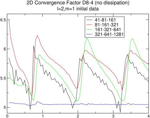
Refer to caption
Figure 22: Simulations of the same equation and initial data as those of the previous figures, except that now the higher order, D8โˆ’4subscript๐ท84D_{8-4} derivative is used and no dissipation has been added.

.

IV.3 Three dimensional simulations

In this application we consider fields propagating on a Kerr black hole background, as governed by equations (56,57,58), with the background metric written in Kerr-Schild form and cubed-sphere coordinates used for the angular directions. Homogeneous maximally dissipative boundary conditions are used at the outer boundary, while no condition is needed at the inner one if it is appropriately placed inside the black hole so that it constitutes a purely-outflow surface.

The Kerr-Schild metric in cubed-sphere coordinates

The Kerr metric in Kerr-Schild form is

dโ€‹s2=ฮทฮผโ€‹ฮฝ+2โ€‹Hโ€‹lฮผโ€‹lฮฝโ€‹dโ€‹xฮผโ€‹dโ€‹xฮฝ๐‘‘superscript๐‘ 2subscript๐œ‚๐œ‡๐œˆ2๐ปsubscript๐‘™๐œ‡subscript๐‘™๐œˆ๐‘‘superscript๐‘ฅ๐œ‡๐‘‘superscript๐‘ฅ๐œˆds^{2}=\eta_{\mu\nu}+2Hl_{\mu}l_{\nu}dx^{\mu}dx^{\nu}

where ฮทฮผโ€‹ฮฝsubscript๐œ‚๐œ‡๐œˆ\eta_{\mu\nu} is the flat metric [with signature (โˆ’,+,+,+)(-,+,+,+)],

H๐ป\displaystyle H =\displaystyle= mโ€‹rr2+A2โ€‹cos2โกฮธ,๐‘š๐‘Ÿsuperscript๐‘Ÿ2superscript๐ด2superscript2๐œƒ\displaystyle\frac{mr}{r^{2}+A^{2}\cos^{2}{\theta}}\,, (59)
r2superscript๐‘Ÿ2\displaystyle r^{2} =\displaystyle= 12โ€‹(ฯ2โˆ’A2)+14โ€‹(ฯ2โˆ’A2)2+A2โ€‹z2,12superscript๐œŒ2superscript๐ด214superscriptsuperscript๐œŒ2superscript๐ด22superscript๐ด2superscript๐‘ง2\displaystyle\frac{1}{2}(\rho^{2}-A^{2})+\sqrt{\frac{1}{4}(\rho^{2}-A^{2})^{2}+A^{2}z^{2}}\,, (60)
ฯ2superscript๐œŒ2\displaystyle\rho^{2} =\displaystyle= x2+y2+z2,superscript๐‘ฅ2superscript๐‘ฆ2superscript๐‘ง2\displaystyle x^{2}+y^{2}+z^{2}\,, (61)

and lฮผsuperscript๐‘™๐œ‡l^{\mu} is a null vector (both with respect to the flat metric and whole metric).

Therefore, in order to write the above metric in cubed-sphere coordinates one needs to write ฮทฮผโ€‹ฮฝsubscript๐œ‚๐œ‡๐œˆ\eta_{\mu\nu} and lฮผsubscript๐‘™๐œ‡l_{\mu} in these coordinates. A straightforward change of coordinates of the first one gives

ฮทฮผโ€‹ฮฝ=โˆ’dโ€‹t2+dโ€‹c2+c2โ€‹Dโˆ’4โ€‹[(1+b2)โ€‹dโ€‹a2+(1+a2)โ€‹dโ€‹b2โˆ’2โ€‹aโ€‹bโ€‹dโ€‹aโ€‹dโ€‹b]subscript๐œ‚๐œ‡๐œˆ๐‘‘superscript๐‘ก2๐‘‘superscript๐‘2superscript๐‘2superscript๐ท4delimited-[]1superscript๐‘2๐‘‘superscript๐‘Ž21superscript๐‘Ž2๐‘‘superscript๐‘22๐‘Ž๐‘๐‘‘๐‘Ž๐‘‘๐‘\eta_{\mu\nu}=-{dt}^{2}+{dc}^{2}+c^{2}D^{-4}\left[(1+b^{2}){da}^{2}+(1+a^{2}){db}^{2}-2a\,b\,{da}\,{db}\right]

with D:=(1+a2+b2)assign๐ท1superscript๐‘Ž2superscript๐‘2D:=\sqrt{(1+a^{2}+b^{2})}.

In Cartesian coordinates the lฮผsubscript๐‘™๐œ‡l_{\mu} co-vector is, in turn,

lโ‰กlฮผโ€‹dโ€‹xฮผ=dโ€‹t+rโ€‹x+Aโ€‹yr2+A2โ€‹dโ€‹x+rโ€‹yโˆ’Aโ€‹xr2+A2โ€‹dโ€‹y+zrโ€‹dโ€‹z๐‘™subscript๐‘™๐œ‡๐‘‘superscript๐‘ฅ๐œ‡๐‘‘๐‘ก๐‘Ÿ๐‘ฅ๐ด๐‘ฆsuperscript๐‘Ÿ2superscript๐ด2๐‘‘๐‘ฅ๐‘Ÿ๐‘ฆ๐ด๐‘ฅsuperscript๐‘Ÿ2superscript๐ด2๐‘‘๐‘ฆ๐‘ง๐‘Ÿ๐‘‘๐‘งl\equiv l_{\mu}dx^{\mu}={dt}+\frac{rx+Ay}{r^{2}+A^{2}}\,{dx}+\frac{ry-Ax}{r^{2}+A^{2}}\,{dy}+\frac{z}{r}\,{dz}

with xฮผ=(t,x,y,z)superscript๐‘ฅ๐œ‡๐‘ก๐‘ฅ๐‘ฆ๐‘งx^{\mu}=(t,x,y,z) which, when changed to cubed-sphere coordinates (t,a,b,c)๐‘ก๐‘Ž๐‘๐‘(t,a,b,c) gives

l๐‘™\displaystyle l =\displaystyle= dโ€‹t+โˆ’c2โ€‹aโ€‹A2โ€‹(a2โˆ’D2)D4โ€‹rโ€‹(r2+A2)โ€‹dโ€‹a+โˆ’c2โ€‹Aโ€‹(D2โ€‹r+Aโ€‹bโ€‹a2)D4โ€‹rโ€‹(r2+A2)โ€‹dโ€‹b+cโ€‹(D2โ€‹r2+a2โ€‹A2)D2โ€‹rโ€‹(r2+A2)โ€‹dโ€‹cโ€‹for patches 0-3๐‘‘๐‘กsuperscript๐‘2๐‘Žsuperscript๐ด2superscript๐‘Ž2superscript๐ท2superscript๐ท4๐‘Ÿsuperscript๐‘Ÿ2superscript๐ด2๐‘‘๐‘Žsuperscript๐‘2๐ดsuperscript๐ท2๐‘Ÿ๐ด๐‘superscript๐‘Ž2superscript๐ท4๐‘Ÿsuperscript๐‘Ÿ2superscript๐ด2๐‘‘๐‘๐‘superscript๐ท2superscript๐‘Ÿ2superscript๐‘Ž2superscript๐ด2superscript๐ท2๐‘Ÿsuperscript๐‘Ÿ2superscript๐ด2๐‘‘๐‘for patches 0-3\displaystyle{dt}+\frac{-c^{2}aA^{2}(a^{2}-D^{2})}{D^{4}r(r^{2}+A^{2})}{da}+\frac{-c^{2}A(D^{2}r+Aba^{2})}{D^{4}r(r^{2}+A^{2})}{db}+\frac{c(D^{2}r^{2}+a^{2}A^{2})}{D^{2}r(r^{2}+A^{2})}{dc}\;\;\;\mbox{for patches 0-3} (62)
l๐‘™\displaystyle l =\displaystyle= dโ€‹t+โˆ’c2โ€‹Aโ€‹(D2โ€‹rโ€‹b+aโ€‹A)D4โ€‹rโ€‹(r2+A2)โ€‹dโ€‹a+c2โ€‹Aโ€‹(rโ€‹aโ€‹D2โˆ’Aโ€‹b)D4โ€‹rโ€‹(r2+A2)โ€‹dโ€‹b+cโ€‹(D2โ€‹r2+A2)D2โ€‹rโ€‹(r2+A2)โ€‹dโ€‹cโ€‹patch 4๐‘‘๐‘กsuperscript๐‘2๐ดsuperscript๐ท2๐‘Ÿ๐‘๐‘Ž๐ดsuperscript๐ท4๐‘Ÿsuperscript๐‘Ÿ2superscript๐ด2๐‘‘๐‘Žsuperscript๐‘2๐ด๐‘Ÿ๐‘Žsuperscript๐ท2๐ด๐‘superscript๐ท4๐‘Ÿsuperscript๐‘Ÿ2superscript๐ด2๐‘‘๐‘๐‘superscript๐ท2superscript๐‘Ÿ2superscript๐ด2superscript๐ท2๐‘Ÿsuperscript๐‘Ÿ2superscript๐ด2๐‘‘๐‘patch 4\displaystyle{dt}+\frac{-c^{2}A(D^{2}rb+aA)}{D^{4}r(r^{2}+A^{2})}{da}+\frac{c^{2}A(raD^{2}-Ab)}{D^{4}r(r^{2}+A^{2})}{db}+\frac{c(D^{2}r^{2}+A^{2})}{D^{2}r(r^{2}+A^{2})}{dc}\;\;\;\mbox{patch 4} (63)
l๐‘™\displaystyle l =\displaystyle= dโ€‹t+โˆ’c2โ€‹Aโ€‹(โˆ’D2โ€‹rโ€‹b+aโ€‹A)D4โ€‹rโ€‹(r2+A2)โ€‹dโ€‹a+โˆ’c2โ€‹Aโ€‹(rโ€‹aโ€‹D2+Aโ€‹b)D4โ€‹rโ€‹(r2+A2)โ€‹dโ€‹b+cโ€‹(D2โ€‹r2+A2)D2โ€‹rโ€‹(r2+A2)โ€‹dโ€‹cโ€‹patch 5๐‘‘๐‘กsuperscript๐‘2๐ดsuperscript๐ท2๐‘Ÿ๐‘๐‘Ž๐ดsuperscript๐ท4๐‘Ÿsuperscript๐‘Ÿ2superscript๐ด2๐‘‘๐‘Žsuperscript๐‘2๐ด๐‘Ÿ๐‘Žsuperscript๐ท2๐ด๐‘superscript๐ท4๐‘Ÿsuperscript๐‘Ÿ2superscript๐ด2๐‘‘๐‘๐‘superscript๐ท2superscript๐‘Ÿ2superscript๐ด2superscript๐ท2๐‘Ÿsuperscript๐‘Ÿ2superscript๐ด2๐‘‘๐‘patch 5\displaystyle{dt}+\frac{-c^{2}A(-D^{2}rb+aA)}{D^{4}r(r^{2}+A^{2})}{da}+\frac{-c^{2}A(raD^{2}+Ab)}{D^{4}r(r^{2}+A^{2})}{db}+\frac{c(D^{2}r^{2}+A^{2})}{D^{2}r(r^{2}+A^{2})}{dc}\;\;\;\mbox{patch 5} (64)

To write the wave equation, one also needs the inverse metric, which is

gฮผโ€‹ฮฝ=ฮทฮผโ€‹ฮฝโˆ’2โ€‹Hโ€‹lฮผโ€‹lฮฝ,superscript๐‘”๐œ‡๐œˆsuperscript๐œ‚๐œ‡๐œˆ2๐ปsuperscript๐‘™๐œ‡superscript๐‘™๐œˆg^{\mu\nu}=\eta^{\mu\nu}-2Hl^{\mu}l^{\nu}\,,

where all indices are raised with ฮทฮผโ€‹ฮฝsuperscript๐œ‚๐œ‡๐œˆ\eta^{\mu\nu} (the inverse of the flat metric). The non-zero components of the latter are:

ฮทaโ€‹asuperscript๐œ‚๐‘Ž๐‘Ž\displaystyle\eta^{aa} =\displaystyle= D2โ€‹(1+a2)c2,superscript๐ท21superscript๐‘Ž2superscript๐‘2\displaystyle\frac{D^{2}(1+a^{2})}{c^{2}}\,, (65)
ฮทbโ€‹bsuperscript๐œ‚๐‘๐‘\displaystyle\eta^{bb} =\displaystyle= D2โ€‹(1+b2)c2,superscript๐ท21superscript๐‘2superscript๐‘2\displaystyle\frac{D^{2}(1+b^{2})}{c^{2}}\,, (66)
ฮทcโ€‹csuperscript๐œ‚๐‘๐‘\displaystyle\eta^{cc} =\displaystyle= 1,1\displaystyle 1\,, (67)
ฮทtโ€‹tsuperscript๐œ‚๐‘ก๐‘ก\displaystyle\eta^{tt} =\displaystyle= โˆ’1,1\displaystyle-1\,, (68)
ฮทaโ€‹bsuperscript๐œ‚๐‘Ž๐‘\displaystyle\eta^{ab} =\displaystyle= aโ€‹bโ€‹D2c2,๐‘Ž๐‘superscript๐ท2superscript๐‘2\displaystyle\frac{abD^{2}}{c^{2}}\,, (69)

and the vector lฮผsuperscript๐‘™๐œ‡l^{\mu} in the cubed-sphere coordinates is,

lฮผsuperscript๐‘™๐œ‡\displaystyle l^{\mu} =\displaystyle= [โˆ’1,โˆ’aโ€‹Aโ€‹(rโ€‹bโˆ’A)rโ€‹(r2+A2),Aโ€‹(a2โˆ’D2)r2+A2,cโ€‹(D2โ€‹r2+a2โ€‹A2)D2โ€‹rโ€‹(r2+A2)]ฮผโ€‹patches 0 to 3superscript1๐‘Ž๐ด๐‘Ÿ๐‘๐ด๐‘Ÿsuperscript๐‘Ÿ2superscript๐ด2๐ดsuperscript๐‘Ž2superscript๐ท2superscript๐‘Ÿ2superscript๐ด2๐‘superscript๐ท2superscript๐‘Ÿ2superscript๐‘Ž2superscript๐ด2superscript๐ท2๐‘Ÿsuperscript๐‘Ÿ2superscript๐ด2๐œ‡patches 0 to 3\displaystyle\left[-1,\frac{-aA(rb-A)}{r(r^{2}+A^{2})},\frac{A(a^{2}-D^{2})}{r^{2}+A^{2}},\frac{c(D^{2}r^{2}+a^{2}A^{2})}{D^{2}r(r^{2}+A^{2})}\right]^{\mu}\;\;\;\mbox{patches 0 to 3} (70)
lฮผsuperscript๐‘™๐œ‡\displaystyle l^{\mu} =\displaystyle= [โˆ’1,โˆ’Aโ€‹(rโ€‹b+aโ€‹A)rโ€‹(r2+A2),Aโ€‹(aโ€‹rโˆ’bโ€‹A)rโ€‹(r2+A2),cโ€‹(D2โ€‹r2+A2)D2โ€‹rโ€‹(r2+A2)]ฮผโ€‹ย for patch 4superscript1๐ด๐‘Ÿ๐‘๐‘Ž๐ด๐‘Ÿsuperscript๐‘Ÿ2superscript๐ด2๐ด๐‘Ž๐‘Ÿ๐‘๐ด๐‘Ÿsuperscript๐‘Ÿ2superscript๐ด2๐‘superscript๐ท2superscript๐‘Ÿ2superscript๐ด2superscript๐ท2๐‘Ÿsuperscript๐‘Ÿ2superscript๐ด2๐œ‡ย for patch 4\displaystyle\left[-1,-\frac{A(rb+aA)}{r(r^{2}+A^{2})},\frac{A(ar-bA)}{r(r^{2}+A^{2})},\frac{c(D^{2}r^{2}+A^{2})}{D^{2}r(r^{2}+A^{2})}\right]^{\mu}\;\;\;\mbox{ for patch 4} (71)
lฮผsuperscript๐‘™๐œ‡\displaystyle l^{\mu} =\displaystyle= [โˆ’1,Aโ€‹(rโ€‹bโˆ’aโ€‹A)rโ€‹(r2+A2),โˆ’Aโ€‹(aโ€‹r+bโ€‹A)rโ€‹(r2+A2),cโ€‹(D2โ€‹r2+A2)D2โ€‹rโ€‹(r2+A2)]ฮผโ€‹ย for patch 5superscript1๐ด๐‘Ÿ๐‘๐‘Ž๐ด๐‘Ÿsuperscript๐‘Ÿ2superscript๐ด2๐ด๐‘Ž๐‘Ÿ๐‘๐ด๐‘Ÿsuperscript๐‘Ÿ2superscript๐ด2๐‘superscript๐ท2superscript๐‘Ÿ2superscript๐ด2superscript๐ท2๐‘Ÿsuperscript๐‘Ÿ2superscript๐ด2๐œ‡ย for patch 5\displaystyle\left[-1,\frac{A(rb-aA)}{r(r^{2}+A^{2})},-\frac{A(ar+bA)}{r(r^{2}+A^{2})},\frac{c(D^{2}r^{2}+A^{2})}{D^{2}r(r^{2}+A^{2})}\right]^{\mu}\mbox{ for patch 5} (72)

IV.3.1 Convergence tests

Figure 23 shows the differences, in the L2subscript๐ฟ2L_{2} norm, between the numerical solutions at consecutive resolutions, using the D8โˆ’4subscript๐ท84D_{8-4} scheme, with no dissipation. The number of points in the angular directions is kept fixed to 16ร—16161616\times 16 points on each of the six patches, and the number of radial points ranges from 101101101 to 640164016401. The background is defined by a non-spinning black hole, and the inner and outer boundaries are at 1.9โ€‹M1.9๐‘€1.9M and 11.9โ€‹M11.9๐‘€11.9M, respectively. Non-trivial initial data is given only to ฮ ฮ \Pi, in the form of a spherically symmetric Gaussian multipole:

ฮ (0,xโ†’)=Aexp(rโˆ’r0)2/ฯƒ02,\Pi(0,\vec{x})=A\exp{(r-r_{0})^{2}/\sigma_{0}^{2}}\,, (74)

with r0=5โ€‹M,ฯƒ=M,A=1formulae-sequencesubscript๐‘Ÿ05๐‘€formulae-sequence๐œŽ๐‘€๐ด1r_{0}=5M,\sigma=M,A=1. The resulting convergence factors, the normalized differences โ€–uNโˆ’u2โ€‹Nโ€–/โ€–uNโ€–normsubscript๐‘ข๐‘subscript๐‘ข2๐‘normsubscript๐‘ข๐‘||u_{N}-u_{2N}||/||u_{N}|| and the non-normalized ones, โ€–uNโˆ’u2โ€‹Nโ€–normsubscript๐‘ข๐‘subscript๐‘ข2๐‘||u_{N}-u_{2N}||, are shown. The use of multiple patches not only allows for non-trivial geometries, but additionally one is able to define coordinates in a way such that resolution is adapted to the problem of interest. For example, in the geometry being considered, S2ร—Rsuperscript๐‘†2๐‘…S^{2}\times R, one employs a number of points in the angular direction limited by the expected multipoles of interest and concentrates resources to increase the number of points in the radial direction. As an example, the relative differences between the solution at different resolutions shown in Figure 23 reaches values close to roundoff, with modest computational resources. Even though the solution here evolved is spherically symmetric at the continuum, as discussed below the number of points used on each of the six patches that cover the sphere can reasonably resolve an l=2๐‘™2l=2 multipole.

Refer to caption
Refer to caption
Refer to caption
Figure 23: Convergence test in the radial direction, with CFL factors ฮป=0.25,0.025๐œ†0.250.025\lambda=0.25,0.025. Notice that no appreciable difference is found between ฮป=0.25๐œ†0.25\lambda=0.25 and a smaller value and even with ฮป=0.25๐œ†0.25\lambda=0.25 the convergence factor is not dominated by the time integrator.

Next, Figure 24 shows similar plots, but keeping the number of radial points fixed (to 101101101), using Naร—Nasubscript๐‘๐‘Žsubscript๐‘๐‘ŽN_{a}\times N_{a} points on each of the six patches in the sphere, with Na=21,41,81subscript๐‘๐‘Ž214181N_{a}=21,41,81.

Refer to caption
Refer to caption
Figure 24: Convergence test in the angular direction, with a CFL factor ฮป=1/4๐œ†14\lambda=1/4

.

IV.3.2 Tail runs

To illustrate the behavior of the described techniques in 333d simulations we examine the propagation of scalar fields on a Kerr black hole background. The numerical undertaking of such problem has been previously treated using pseudo-spectral methods tail_spectral , which for smooth solutions allows the construction of very efficient schemes. As explained next, the combination of multi-block evolutions with high order schemes also lets one to treat the problem quite efficiently. A detailed study of this problem will be presented elsewhere nils ; we here concentrate on two representative examples of what is achievable.

In the first case we examine the behavior of the scalar field propagating on a background defined by a black hole with mass M=1๐‘€1M=1 and spin parameter a=0.5๐‘Ž0.5a=0.5. Non trivial initial data is given only to ฮ ฮ \Pi, with a radial profile given by a Gaussian pulse as in Eq.(74) and angular dependence given by a pure l=2๐‘™2l=2 multipole. The inner and outer boundaries are placed at r=1.8โ€‹M๐‘Ÿ1.8๐‘€r=1.8M and r=1001.8โ€‹M๐‘Ÿ1001.8๐‘€r=1001.8M respectively. We adopt a grid composed by six cubed-sphere patches, each of which is discretized with 20ร—20202020\times 20 points in the angular directions and 100011000110001 points in the radial one. This translates into a relatively inexpensive calculation.

We adopt the D8โˆ’4subscript๐ท84D_{8-4} derivative operator, add no artificial dissipation and choose a CFL factor ฮป=0.25๐œ†0.25\lambda=0.25. The salient features of the solutionโ€™s behavior observed are summarized in figure 25 which shows the the time derivative of the scalar field, as a function of time, at a point in the equatorial plane, on the even horizon. At earlier stages, the familiar quasi-normal ringing is observed. Next the late-time behavior of the field reveals the expected tail-behavior as a fit in the interval tโˆˆ[350โ€‹M,750โ€‹M]๐‘ก350๐‘€750๐‘€t\in[350M,750M] gives a decay for ฮ ฮ \Pi of tโˆ’4.07superscript๐‘ก4.07t^{-4.07}, which agrees quite well the expected decay of tโˆ’4superscript๐‘ก4t^{-4}. This can be understood in terms of the generation of an l=0๐‘™0l=0 mode in the solution due to the spin of the black hole tail_spectral ; burko-khanna . Finally, noise can be observed appearing at tโ‰ˆ800โ€‹M๐‘ก800๐‘€t\approx 800M due to the outer boundary. This noise, however, is not related to physical information propagating to the outer boundary and coming back (for this one would have to wait till tโ‰ˆ2,000โ€‹M๐‘ก2000๐‘€t\approx 2,000M) but, rather, is related to spurious modes with high group velocities traveling in the wrong direction, as described in Section III. As discussed there, for an eighth order centered derivative the speed of this spurious mode is around โˆ’2.62.6-2.6, which roughly matches with this noise appearing at tโ‰ˆ800โ€‹M๐‘ก800๐‘€t\approx 800M. We have checked that this boundary effect does go away with resolution, by introducing some amount of dissipation or by pushing the outer boundary farther out. Notice that while the first two options allow one to observe the tail behavior for much longer, eventually physical information would travel back from the outer boundary and โ€œcavityโ€ effects which affect the decay would take place. Indeed, the behavior would no longer be determined by a power law tail but by an exponential decay priceburko .
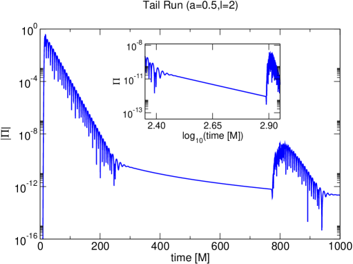
Refer to caption
Figure 25: Behavior of the time derivative of the scalar field for a pure multipole l=2๐‘™2l=2 initial data, on a Kerr background, with a=0.5๐‘Ž0.5a=0.5. Inner and outer boundaries are at 1.8โ€‹M1.8๐‘€1.8M and 1,001.8โ€‹M1001.8๐‘€1,001.8M, respectively and the six-patches grid is covered by 20ร—20ร—10,00120201000120\times 20\times 10,001 points on each patch. The D8โˆ’4subscript๐ท84D_{8-4} derivative is used, with no artificial dissipation. The noise at tโ‰ˆ800โ€‹M๐‘ก800๐‘€t\approx 800M is due to the mode with group speed โˆ’2.62.6-2.6 discussed in Section III hitting the outer boundary and reaching the observer at the black hole horizon. This noise goes away by either pushing the outer boundary, increasing resolution and/or adding dissipation. The average slope for ฮ ฮ \Pi in the interval tโˆˆ[350โ€‹M,750โ€‹M]๐‘ก350๐‘€750๐‘€t\in[350M,750M] gives a decay for ฮ ฮ \Pi of tโˆ’4.07superscript๐‘ก4.07t^{-4.07}, in good agreement with the expected decay of tโˆ’4superscript๐‘ก4t^{-4}. The inset shows a zoom in at the tail behavior.

Figure 26 shows a similar run, in this case however the black is not spinning. A fit to the solution in the tail regime gives a decay for ฯ•italic-ฯ•\phi of tโˆ’6.96superscript๐‘ก6.96t^{-6.96}, which again matches quite well the expected decay of tโˆ’7superscript๐‘ก7t^{-7} price .

Refer to caption
Figure 26: A simulation with the same parameters as those of Fig. 25, but with a non-spinning black hole. The average slope for ฮฆฮฆ\Phi in tail regime gives a decay of tโˆ’6.96superscript๐‘ก6.96t^{-6.96}, again in good agreement with the expected decay of tโˆ’7superscript๐‘ก7t^{-7}.

V Final Comments

As illustrated in this work, the combination of the penalty technique together with those guaranteeing a stable single grid implementation for hyperbolic systems provides a way to achieve stable implementations of multi-block schemes of arbitrary high order. A similar penalty technique for multi-block evolutions is also being pursued in conjuction with pseudo-spectral methods kps .

The flexibility provided by multiple grids can be exploited to address a number of issues currently faced in simulations of Einsteinโ€™s equations, among these

  • โ€ข

    The desire for a conforming inner boundary. This plays a central role in ensuring a consistent implementation of the excision technique together with a saving in the computational cost of the implementation.

  • โ€ข

    The need for a smooth outer boundary. This removes the presence of corners and edges which have proved difficult to dealt with even at the analytical level ibv ; gioel . Furthermore, a smooth S2superscript๐‘†2S^{2} outer boundary simplifies tremendously the search for an efficient matching strategy to an outside formulation aimed to cover a much larger region of the spacetime with a formalism better suited to the asymptotic region (see, for example, ccm and cpm1 ; cpm2 ; cpm3 ).

  • โ€ข

    The use of a grid that is better adapted to the description of wave phenomena as they propagate in the region far from the sources.

VI Acknowledgments

This research was supported in part by the NSF under Grants No PHY0244335, PHY0244699, PHY0326311, INT0204937, and PHY0505761 to Louisiana State University, No. PHY0354631 and PHY0312072 to Cornell University, No PHY9907949 to the University of California as Santa Barbara; the Horace Hearne Jr. Institute for Theoretical Physics; CONICET and SECYT-UNC. This research employed the resources of the Center for Computation and Technology at Louisiana State University, which is supported by funding from the Louisiana legislatureโ€™s Information Technology Initiative. L. L. was partially supported by the Alfred P. Sloan Foundation.

We thank Mark Carpenter, Peter Diener, Nils Dorband, Ian Hawke, Larry Kidder, Ken Mattsson, Jorge Pullin, Olivier Sarbach, Erik Schnetter, Magnus Svard, Saul Teukolsky, Jonathan Thornburg, and Burkhard Zink for helpful discussions, suggestions and/or comments on the manuscript.

The authors thank Louisiana State University and the Horace Hearne Jr. Institute for Theoretical Physics, the Universidad Nacional de Cordoba and FaMAF, and the University of California at Santa Barbara for hospitality at different stages of this work.

Appendix A Coefficients for high order operators with diagonal metrics

For completeness we point out here some misprints in Ref.strand in some of the expressions for the diagonal metric cases.

  • โ€ข

    D2โˆ’1subscript๐ท21D_{2-1}: No typos.

  • โ€ข

    D4โˆ’2subscript๐ท42D_{4-2}: It says ฮฑ2=โˆ’1/2subscript๐›ผ212\alpha_{2}=-1/2, but it should be ฮฑ2=โˆ’1/12subscript๐›ผ2112\alpha_{2}=-1/12. The expressions for q2โ€‹isubscript๐‘ž2๐‘–q_{2i} are also missing; they should be the following:

    q20=886=q21=โˆ’5986=q23=โˆ’q21,q24=โˆ’q20formulae-sequencesubscript๐‘ž20886subscript๐‘ž215986subscript๐‘ž23subscript๐‘ž21subscript๐‘ž24subscript๐‘ž20q_{20}=\frac{8}{86}\;\;\;=\;\;\;q_{21}=-\frac{59}{86}\;\;\;=\;\;\;q_{23}=-q_{21}\;\;\;,\;\;\;q_{24}=-q_{20}
  • โ€ข

    D6โˆ’3subscript๐ท63D_{6-3}: No typos in the scalar product or coefficients for the derivative, neither in the general case nor in the minimum bandwidth one.

  • โ€ข

    D8โˆ’4subscript๐ท84D_{8-4}: The operator that has the minimum bandwidth is correct, but the three-parametric one has a typo in one of the coefficients (the scalar product is correct): it says

    q06=49โ€‹(โˆ’1244160โ€‹x1+18661400โ€‹x3โˆ’13322233)/17977668subscript๐‘ž06491244160subscript๐‘ฅ118661400subscript๐‘ฅ31332223317977668q_{06}=49(-1244160x_{1}+18661400x_{3}-13322233)/17977668

    when it should say

    q06=49โ€‹(โˆ’1244160โ€‹x1+18662400โ€‹x3โˆ’13322233)/17977668subscript๐‘ž06491244160subscript๐‘ฅ118662400subscript๐‘ฅ31332223317977668q_{06}=49(-1244160x_{1}+18662400x_{3}-13322233)/17977668

Appendix B Dissipation for high order difference operators with diagonal norms

The addition of artificial dissipation typically involves considering a dissipative operator Qdsubscript๐‘„๐‘‘Q_{d} which is non-positive with respect to the scalar product with respect to which SBP holds, i.e.,

<u,Qdu>โ‰ค0โˆ€u.<u,Q_{d}u>\leq 0\;\;\;\forall u\;. (75)

We start the construction of such operators satisfying this property by defining them as

Qd=(โˆ’1)mโˆ’1โ€‹ฯƒโ€‹hnโ€‹(D+โ€‹Dโˆ’)msubscript๐‘„๐‘‘superscript1๐‘š1๐œŽsuperscriptโ„Ž๐‘›superscriptsubscript๐ทsubscript๐ท๐‘šQ_{d}=(-1)^{m-1}\sigma h^{n}(D_{+}D_{-})^{m} (76)

on gridpoints lying within the range [r,s]๐‘Ÿ๐‘ [r,s] contained in the interval in which the weight used in the scalar product is one. That is, the interval in which the difference operator is one of the centered ones of Eqs.(30,31,32,33); for example, if the gridpoints range from 00 to N๐‘N, then (r,s)๐‘Ÿ๐‘ (r,s) must satisfy

rโ‰ฅ1,sโ‰คNโˆ’1โ€‹ย forย โ€‹D2โˆ’1;formulae-sequence๐‘Ÿ1๐‘ ๐‘1ย forย subscript๐ท21r\geq 1,s\leq N-1\;\;\;\mbox{ for }D_{2-1}\,; (77)
rโ‰ฅ4,sโ‰คNโˆ’4โ€‹ย forย โ€‹D4โˆ’2;formulae-sequence๐‘Ÿ4๐‘ ๐‘4ย forย subscript๐ท42r\geq 4,s\leq N-4\;\;\;\mbox{ for }D_{4-2}\,; (78)
rโ‰ฅ6,sโ‰คNโˆ’6โ€‹ย forย โ€‹D6โˆ’3;formulae-sequence๐‘Ÿ6๐‘ ๐‘6ย forย subscript๐ท63r\geq 6,s\leq N-6\;\;\;\mbox{ for }D_{6-3}\,; (79)
rโ‰ฅ8,sโ‰คNโˆ’8โ€‹ย forย โ€‹D8โˆ’4.formulae-sequence๐‘Ÿ8๐‘ ๐‘8ย forย subscript๐ท84r\geq 8,s\leq N-8\;\;\;\mbox{ for }D_{8-4}\,. (80)

As we will see later, in some cases our construction of dissipative operators imposes stricter constraints on the range of allowed values for r,s๐‘Ÿ๐‘ r,s for each derivative.

If n=2โ€‹mโˆ’1๐‘›2๐‘š1n=2m-1, the operator (76) is the standard Kreissโ€“Oliger dissipation (KO) ko , which is negative definite in the absence of boundaries (when the weight in the scalar product is identically one). The choice n=2โ€‹mโˆ’1๐‘›2๐‘š1n=2m-1 ensures that the added dissipation has the same โ€˜scaleโ€™ as the principal part (that is, length-1) and that the resulting amplification factor is independent of resolution.

For each of the derivatives D2โˆ’1,D4โˆ’2,D6โˆ’3,D8โˆ’4subscript๐ท21subscript๐ท42subscript๐ท63subscript๐ท84D_{2-1},D_{4-2},D_{6-3},D_{8-4}, we seek to extend Qdsubscript๐‘„๐‘‘Q_{d} in Eq.(76) so that the resulting operator is negative definite with respect to the corresponding SBP scalar product. As mentioned above, we denote the points in which Qdsubscript๐‘„๐‘‘Q_{d} is given by Eq.(76) as i=rโ€‹โ€ฆโ€‹s๐‘–๐‘Ÿโ€ฆ๐‘ i=r\ldots s.

The identities of Appendix C are used in the calculations needed for the construction of the operators below. These identities let one express the norm of the dissipation in the interior, which is proportional to (โˆ’1)nโˆ’1โ€‹(u,(D+โ€‹Dโˆ’)nโ€‹u)[r,s]superscript1๐‘›1superscript๐‘ขsuperscriptsubscript๐ทsubscript๐ท๐‘›๐‘ข๐‘Ÿ๐‘ (-1)^{n-1}(u,(D_{+}D_{-})^{n}u)^{[r,s]}, as

(โˆ’1)nโˆ’1โ€‹(u,(D+โ€‹Dโˆ’)nโ€‹u)[r,s]=non-positive definite terms+โˆ‘0rโˆ’1uiโ€‹(โ€ฆ)+โˆ‘s+1Nuiโ€‹(โ€ฆ).superscript1๐‘›1superscript๐‘ขsuperscriptsubscript๐ทsubscript๐ท๐‘›๐‘ข๐‘Ÿ๐‘ non-positive definite termssuperscriptsubscript0๐‘Ÿ1subscript๐‘ข๐‘–โ€ฆsuperscriptsubscript๐‘ 1๐‘subscript๐‘ข๐‘–โ€ฆ(-1)^{n-1}(u,(D_{+}D_{-})^{n}u)^{[r,s]}=\mbox{non-positive definite terms}+\sum_{0}^{r-1}u_{i}(\ldots)+\sum_{s+1}^{N}u_{i}(\ldots)\,. (81)

Once this is done, the norm of the whole dissipative operator can be written as

(u,Qdโ€‹u)[0,N]=non-positive definite terms+โˆ‘0rโˆ’1uiโ€‹[(โ€ฆ)i+hโ€‹ฯƒiโ€‹Qdโ€‹ui]+โˆ‘s+1Nuiโ€‹[(โ€ฆ)i+hโ€‹ฯƒiโ€‹Qdโ€‹ui]superscript๐‘ขsubscript๐‘„๐‘‘๐‘ข0๐‘non-positive definite termssuperscriptsubscript0๐‘Ÿ1subscript๐‘ข๐‘–delimited-[]subscriptโ€ฆ๐‘–โ„Žsubscript๐œŽ๐‘–subscript๐‘„๐‘‘subscript๐‘ข๐‘–superscriptsubscript๐‘ 1๐‘subscript๐‘ข๐‘–delimited-[]subscriptโ€ฆ๐‘–โ„Žsubscript๐œŽ๐‘–subscript๐‘„๐‘‘subscript๐‘ข๐‘–(u,Q_{d}u)^{[0,N]}=\mbox{non-positive definite terms}+\sum_{0}^{r-1}u_{i}[(\ldots)_{i}+h\sigma_{i}Q_{d}u_{i}]+\sum_{s+1}^{N}u_{i}[(\ldots)_{i}+h\sigma_{i}Q_{d}u_{i}] (82)

and it is straightforward to make it non-positive definite. For example, by choosing

Qdโ€‹ui=โˆ’(โ€ฆ)iฯƒiโ€‹h,subscript๐‘„๐‘‘subscript๐‘ข๐‘–subscriptโ€ฆ๐‘–subscript๐œŽ๐‘–โ„ŽQ_{d}u_{i}=-\frac{(\ldots)_{i}}{\sigma_{i}h}\;, (83)

which is how we proceed below. Notice however this is not the only way to proceed. For instance, one could try to make the two sums of Eq.(82) cancel (as opposed to requiring the terms cancel at each gridpoint).

A more general approach for constructing dissipative operators that are negative definite with respect to the appropriate (SBP) scalar product has been recently presented by Mattson, Svard and Nordstrom mattsson .

B.1 Fourth derivative dissipation, and KO type for D2โˆ’1subscript๐ท21D_{2-1}

In this case the interior operator is

Qd=โˆ’ฯƒโ€‹hnโ€‹(D+โ€‹Dโˆ’)2.subscript๐‘„๐‘‘๐œŽsuperscriptโ„Ž๐‘›superscriptsubscript๐ทsubscript๐ท2Q_{d}=-\sigma h^{n}(D_{+}D_{-})^{2}\,.

One can then split the norm of the dissipative operator over the whole grid into terms involving the left and right ranges [0,r],[s,N]0๐‘Ÿ๐‘ ๐‘[0,r],[s,N] (of the yet undefined operator) and the interior terms:

(u,Qdโ€‹u)ฮฃ[0,N]=hโ€‹โˆ‘0rโˆ’1ฯƒiโ€‹uiโ€‹Qdโ€‹ui+hโ€‹โˆ‘s+1Nฯƒiโ€‹uiโ€‹Qdโ€‹uiโˆ’ฯƒโ€‹hnโ€‹(u,(D+โ€‹Dโˆ’)2)[r,s]superscriptsubscript๐‘ขsubscript๐‘„๐‘‘๐‘ขฮฃ0๐‘โ„Žsuperscriptsubscript0๐‘Ÿ1subscript๐œŽ๐‘–subscript๐‘ข๐‘–subscript๐‘„๐‘‘subscript๐‘ข๐‘–โ„Žsuperscriptsubscript๐‘ 1๐‘subscript๐œŽ๐‘–subscript๐‘ข๐‘–subscript๐‘„๐‘‘subscript๐‘ข๐‘–๐œŽsuperscriptโ„Ž๐‘›superscript๐‘ขsuperscriptsubscript๐ทsubscript๐ท2๐‘Ÿ๐‘ (u,Q_{d}u)_{\Sigma}^{[0,N]}=h\sum_{0}^{r-1}\sigma_{i}u_{i}Q_{d}u_{i}+h\sum_{s+1}^{N}\sigma_{i}u_{i}Q_{d}u_{i}-\sigma h^{n}(u,(D_{+}D_{-})^{2})^{[r,s]}

where ฯƒisubscript๐œŽ๐‘–\sigma_{i} are the scalar product weights. Using the identities of Appendix C One can see that

(u,Qdโ€‹u)ฮฃ[0,N]superscriptsubscript๐‘ขsubscript๐‘„๐‘‘๐‘ขฮฃ0๐‘\displaystyle(u,Q_{d}u)_{\Sigma}^{[0,N]} =\displaystyle= โˆ’ฯƒโ€‹hnโ€‹โ€–D+โ€‹Dโˆ’โ€‹uโ€–[rโˆ’1,s+1]2+hโ€‹โˆ‘0rโˆ’3ฯƒiโ€‹uiโ€‹Qdโ€‹ui+hโ€‹โˆ‘s+3Nฯƒiโ€‹uiโ€‹Qdโ€‹ui๐œŽsuperscriptโ„Ž๐‘›subscriptsuperscriptnormsubscript๐ทsubscript๐ท๐‘ข2๐‘Ÿ1๐‘ 1โ„Žsuperscriptsubscript0๐‘Ÿ3subscript๐œŽ๐‘–subscript๐‘ข๐‘–subscript๐‘„๐‘‘subscript๐‘ข๐‘–โ„Žsuperscriptsubscript๐‘ 3๐‘subscript๐œŽ๐‘–subscript๐‘ข๐‘–subscript๐‘„๐‘‘subscript๐‘ข๐‘–\displaystyle-\sigma h^{n}||D_{+}D_{-}u||^{2}_{[r-1,s+1]}+h\sum_{0}^{r-3}\sigma_{i}u_{i}Q_{d}u_{i}+h\sum_{s+3}^{N}\sigma_{i}u_{i}Q_{d}u_{i}
+hurโˆ’2(ฯƒrโˆ’2Qd+ฯƒhnโˆ’2D+2)urโˆ’2+hurโˆ’1[ฯƒrโˆ’1Qdโˆ’ฯƒhnโˆ’2(2D+Dโˆ’โˆ’D+2])urโˆ’1\displaystyle+hu_{r-2}\left(\sigma_{r-2}Q_{d}+\sigma h^{n-2}D_{+}^{2}\right)u_{r-2}+hu_{r-1}\left[\sigma_{r-1}Q_{d}-\sigma h^{n-2}(2D_{+}D_{-}-D_{+}^{2}]\right)u_{r-1}
+hโ€‹us+2โ€‹(ฯƒs+2โ€‹Qd+ฯƒโ€‹hnโˆ’2โ€‹Dโˆ’2)โ€‹us+2+hโ€‹us+1โ€‹[ฯƒs+1โ€‹Qdโˆ’ฯƒโ€‹hnโˆ’2โ€‹(2โ€‹D+โ€‹Dโˆ’โˆ’Dโˆ’2)]โ€‹us+1โ„Žsubscript๐‘ข๐‘ 2subscript๐œŽ๐‘ 2subscript๐‘„๐‘‘๐œŽsuperscriptโ„Ž๐‘›2superscriptsubscript๐ท2subscript๐‘ข๐‘ 2โ„Žsubscript๐‘ข๐‘ 1delimited-[]subscript๐œŽ๐‘ 1subscript๐‘„๐‘‘๐œŽsuperscriptโ„Ž๐‘›22subscript๐ทsubscript๐ทsuperscriptsubscript๐ท2subscript๐‘ข๐‘ 1\displaystyle+hu_{s+2}\left(\sigma_{s+2}Q_{d}+\sigma h^{n-2}D_{-}^{2}\right)u_{s+2}+hu_{s+1}\left[\sigma_{s+1}Q_{d}-\sigma h^{n-2}(2D_{+}D_{-}-D_{-}^{2})\right]u_{s+1}

There are several options now to control the contribution of these terms, the simplest one is

Qdโ€‹urโˆ’2subscript๐‘„๐‘‘subscript๐‘ข๐‘Ÿ2\displaystyle Q_{d}u_{r-2} =\displaystyle= โˆ’ฯƒโ€‹hnโˆ’2ฯƒrโˆ’2โ€‹D+2โ€‹urโˆ’2๐œŽsuperscriptโ„Ž๐‘›2subscript๐œŽ๐‘Ÿ2superscriptsubscript๐ท2subscript๐‘ข๐‘Ÿ2\displaystyle-\frac{\sigma h^{n-2}}{\sigma_{r-2}}D_{+}^{2}u_{r-2}
Qdโ€‹urโˆ’1subscript๐‘„๐‘‘subscript๐‘ข๐‘Ÿ1\displaystyle Q_{d}u_{r-1} =\displaystyle= ฯƒโ€‹hnโˆ’2ฯƒrโˆ’1โ€‹(2โ€‹D+โ€‹Dโˆ’โˆ’D+2)โ€‹urโˆ’1๐œŽsuperscriptโ„Ž๐‘›2subscript๐œŽ๐‘Ÿ12subscript๐ทsubscript๐ทsuperscriptsubscript๐ท2subscript๐‘ข๐‘Ÿ1\displaystyle\frac{\sigma h^{n-2}}{\sigma_{r-1}}(2D_{+}D_{-}-D_{+}^{2})u_{r-1}
Qdโ€‹us+1subscript๐‘„๐‘‘subscript๐‘ข๐‘ 1\displaystyle Q_{d}u_{s+1} =\displaystyle= ฯƒโ€‹hnโˆ’2ฯƒs+1โ€‹(2โ€‹D+โ€‹Dโˆ’โˆ’Dโˆ’2)โ€‹us+1๐œŽsuperscriptโ„Ž๐‘›2subscript๐œŽ๐‘ 12subscript๐ทsubscript๐ทsuperscriptsubscript๐ท2subscript๐‘ข๐‘ 1\displaystyle\frac{\sigma h^{n-2}}{\sigma_{s+1}}(2D_{+}D_{-}-D_{-}^{2})u_{s+1}
Qdโ€‹us+2subscript๐‘„๐‘‘subscript๐‘ข๐‘ 2\displaystyle Q_{d}u_{s+2} =\displaystyle= โˆ’2โ€‹ฯƒฯƒs+2โ€‹hnโˆ’2โ€‹Dโˆ’2โ€‹us+22๐œŽsubscript๐œŽ๐‘ 2superscriptโ„Ž๐‘›2superscriptsubscript๐ท2subscript๐‘ข๐‘ 2\displaystyle-\frac{2\sigma}{\sigma_{s+2}}h^{n-2}D_{-}^{2}u_{s+2}

and Qd=0subscript๐‘„๐‘‘0Q_{d}=0 everywhere else, which implies rโ‰ฅ2,sโ‰คNโˆ’2formulae-sequence๐‘Ÿ2๐‘ ๐‘2r\geq 2,s\leq N-2. Notice that, as anticipated, this is a further constraint on the possible range of r,s๐‘Ÿ๐‘ r,s [c.f. Eq.(77)]. The operator constructed not only satisfies the non-positivity requirement, but also transforms according to Dโˆ’โ†’โˆ’D+โ†’subscript๐ทsubscript๐ทD_{-}\rightarrow-D_{+} under the symmetry iโˆ’โ†’Nโˆ’iโ†’limit-from๐‘–๐‘๐‘–i-\rightarrow N-i (as it should).

Preferred choice:

A KO type dissipation for D2โˆ’1subscript๐ท21D_{2-1}, which we call KO4 (because it involves fourth derivatives in the interior) corresponds to

n=3.๐‘›3n=3\;.

With this choice the order of the scheme is one in at least two points (while in the absence of dissipation would be of order one in just one point). In general, the best option for r,s๐‘Ÿ๐‘ r,s is

r=2,s=Nโˆ’2,formulae-sequence๐‘Ÿ2๐‘ ๐‘2r=2,s=N-2\;,

as in that case the dissipation operator is non-trivial everywhere (while choosing r>2,s<Nโˆ’2formulae-sequence๐‘Ÿ2๐‘ ๐‘2r>2,s<N-2 would imply that the dissipation is zero at โ€“and even possibly close toโ€“ the boundaries). With this choice for r,s๐‘Ÿ๐‘ r,s the order of the scheme is one at the last two boundary points.

B.2 Sixth derivative dissipation, and KO type for D4โˆ’2subscript๐ท42D_{4-2}

We now proceed to construct a higher derivative dissipative operator. As before, we adopt at the interior points the standard dissipation operator,

Qd=ฯƒโ€‹hnโ€‹D+3โ€‹Dโˆ’3subscript๐‘„๐‘‘๐œŽsuperscriptโ„Ž๐‘›superscriptsubscript๐ท3superscriptsubscript๐ท3Q_{d}=\sigma h^{n}D_{+}^{3}D_{-}^{3}

Then, defining v=D+โ€‹Dโˆ’โ€‹u๐‘ฃsubscript๐ทsubscript๐ท๐‘ขv=D_{+}D_{-}u and employing the identities of Appendix C one obtains

(u,Qdโ€‹u)ฮฃ[0,N]superscriptsubscript๐‘ขsubscript๐‘„๐‘‘๐‘ขฮฃ0๐‘\displaystyle(u,Q_{d}u)_{\Sigma}^{[0,N]} =\displaystyle= โˆ’ฯƒโ€‹hnโ€‹โ€–Dโˆ’โ€‹vโ€–[rโˆ’1,s+2]2+hโ€‹โˆ‘0rโˆ’1ฯƒiโ€‹uiโ€‹Qdโ€‹ui+hโ€‹โˆ‘s+1Nฯƒiโ€‹uiโ€‹Qdโ€‹ui๐œŽsuperscriptโ„Ž๐‘›subscriptsuperscriptnormsubscript๐ท๐‘ฃ2๐‘Ÿ1๐‘ 2โ„Žsuperscriptsubscript0๐‘Ÿ1subscript๐œŽ๐‘–subscript๐‘ข๐‘–subscript๐‘„๐‘‘subscript๐‘ข๐‘–โ„Žsuperscriptsubscript๐‘ 1๐‘subscript๐œŽ๐‘–subscript๐‘ข๐‘–subscript๐‘„๐‘‘subscript๐‘ข๐‘–\displaystyle-\sigma h^{n}||D_{-}v||^{2}_{[r-1,s+2]}+h\sum_{0}^{r-1}\sigma_{i}u_{i}Q_{d}u_{i}+h\sum_{s+1}^{N}\sigma_{i}u_{i}Q_{d}u_{i}
+urโˆ’3โ€‹hโ€‹(โˆ’ฯƒโ€‹hnโˆ’3โ€‹D+โ€‹vrโˆ’2+ฯƒrโˆ’3โ€‹Qdโ€‹urโˆ’3)subscript๐‘ข๐‘Ÿ3โ„Ž๐œŽsuperscriptโ„Ž๐‘›3subscript๐ทsubscript๐‘ฃ๐‘Ÿ2subscript๐œŽ๐‘Ÿ3subscript๐‘„๐‘‘subscript๐‘ข๐‘Ÿ3\displaystyle+u_{r-3}h\left(-\sigma h^{n-3}D_{+}v_{r-2}+\sigma_{r-3}Q_{d}u_{r-3}\right)
+urโˆ’2โ€‹hโ€‹(ฯƒโ€‹hnโˆ’3โ€‹(โˆ’hโ€‹D+2+2โ€‹D+)โ€‹vrโˆ’2+ฯƒrโˆ’2โ€‹Qdโ€‹urโˆ’2)subscript๐‘ข๐‘Ÿ2โ„Ž๐œŽsuperscriptโ„Ž๐‘›3โ„Žsuperscriptsubscript๐ท22subscript๐ทsubscript๐‘ฃ๐‘Ÿ2subscript๐œŽ๐‘Ÿ2subscript๐‘„๐‘‘subscript๐‘ข๐‘Ÿ2\displaystyle+u_{r-2}h\left(\sigma h^{n-3}(-hD_{+}^{2}+2D_{+})v_{r-2}+\sigma_{r-2}Q_{d}u_{r-2}\right)
+urโˆ’1โ€‹hโ€‹[ฯƒโ€‹hnโˆ’3โ€‹(hโ€‹(2โ€‹D+โ€‹Dโˆ’โˆ’D+2)โ€‹vrโˆ’1โˆ’D+โ€‹vrโˆ’2)+ฯƒrโˆ’1โ€‹Qdโ€‹urโˆ’1]+limit-fromsubscript๐‘ข๐‘Ÿ1โ„Ždelimited-[]๐œŽsuperscriptโ„Ž๐‘›3โ„Ž2subscript๐ทsubscript๐ทsuperscriptsubscript๐ท2subscript๐‘ฃ๐‘Ÿ1subscript๐ทsubscript๐‘ฃ๐‘Ÿ2subscript๐œŽ๐‘Ÿ1subscript๐‘„๐‘‘subscript๐‘ข๐‘Ÿ1\displaystyle+u_{r-1}h\left[\sigma h^{n-3}\left(h(2D_{+}D_{-}-D_{+}^{2})v_{r-1}-D_{+}v_{r-2}\right)+\sigma_{r-1}Q_{d}u_{r-1}\right]+
+us+1โ€‹hโ€‹[ฯƒโ€‹hnโˆ’3โ€‹(hโ€‹(2โ€‹D+โ€‹Dโˆ’โˆ’Dโˆ’2)โ€‹vs+1+Dโˆ’โ€‹vs+2)+ฯƒs+1โ€‹Qdโ€‹us+1]subscript๐‘ข๐‘ 1โ„Ždelimited-[]๐œŽsuperscriptโ„Ž๐‘›3โ„Ž2subscript๐ทsubscript๐ทsuperscriptsubscript๐ท2subscript๐‘ฃ๐‘ 1subscript๐ทsubscript๐‘ฃ๐‘ 2subscript๐œŽ๐‘ 1subscript๐‘„๐‘‘subscript๐‘ข๐‘ 1\displaystyle+u_{s+1}h\left[\sigma h^{n-3}\left(h(2D_{+}D_{-}-D_{-}^{2})v_{s+1}+D_{-}v_{s+2}\right)+\sigma_{s+1}Q_{d}u_{s+1}\right]
+us+2โ€‹hโ€‹(ฯƒโ€‹hnโˆ’3โ€‹(โˆ’hโ€‹Dโˆ’2โˆ’2โ€‹Dโˆ’)โ€‹vs+2+ฯƒs+2โ€‹Qdโ€‹us+2)subscript๐‘ข๐‘ 2โ„Ž๐œŽsuperscriptโ„Ž๐‘›3โ„Žsuperscriptsubscript๐ท22subscript๐ทsubscript๐‘ฃ๐‘ 2subscript๐œŽ๐‘ 2subscript๐‘„๐‘‘subscript๐‘ข๐‘ 2\displaystyle+u_{s+2}h\left(\sigma h^{n-3}(-hD_{-}^{2}-2D_{-})v_{s+2}+\sigma_{s+2}Q_{d}u_{s+2}\right)
+us+3โ€‹hโ€‹(ฯƒโ€‹hnโˆ’3โ€‹Dโˆ’โ€‹vs+2+ฯƒs+3โ€‹Qdโ€‹us+3).subscript๐‘ข๐‘ 3โ„Ž๐œŽsuperscriptโ„Ž๐‘›3subscript๐ทsubscript๐‘ฃ๐‘ 2subscript๐œŽ๐‘ 3subscript๐‘„๐‘‘subscript๐‘ข๐‘ 3\displaystyle+u_{s+3}h\left(\sigma h^{n-3}D_{-}v_{s+2}+\sigma_{s+3}Q_{d}u_{s+3}\right)\,.

Here again one has several options, the simplest one is:

Qdโ€‹urโˆ’3subscript๐‘„๐‘‘subscript๐‘ข๐‘Ÿ3\displaystyle Q_{d}u_{r-3} =\displaystyle= ฯƒโ€‹hnโˆ’3ฯƒrโˆ’3โ€‹D+โ€‹vrโˆ’2๐œŽsuperscriptโ„Ž๐‘›3subscript๐œŽ๐‘Ÿ3subscript๐ทsubscript๐‘ฃ๐‘Ÿ2\displaystyle\frac{\sigma h^{n-3}}{\sigma_{r-3}}D_{+}v_{r-2}
Qdโ€‹urโˆ’2subscript๐‘„๐‘‘subscript๐‘ข๐‘Ÿ2\displaystyle Q_{d}u_{r-2} =\displaystyle= ฯƒโ€‹hnโˆ’2ฯƒrโˆ’2โ€‹(hโ€‹D+2โˆ’2โ€‹D+)โ€‹vrโˆ’2๐œŽsuperscriptโ„Ž๐‘›2subscript๐œŽ๐‘Ÿ2โ„Žsuperscriptsubscript๐ท22subscript๐ทsubscript๐‘ฃ๐‘Ÿ2\displaystyle\frac{\sigma h^{n-2}}{\sigma_{r-2}}(hD_{+}^{2}-2D_{+})v_{r-2}
Qdโ€‹urโˆ’1subscript๐‘„๐‘‘subscript๐‘ข๐‘Ÿ1\displaystyle Q_{d}u_{r-1} =\displaystyle= โˆ’ฯƒโ€‹hnโˆ’2ฯƒrโˆ’1โ€‹[hโ€‹(2โ€‹D+โ€‹Dโˆ’โˆ’D+2)โ€‹vrโˆ’1โˆ’D+โ€‹vrโˆ’2]๐œŽsuperscriptโ„Ž๐‘›2subscript๐œŽ๐‘Ÿ1delimited-[]โ„Ž2subscript๐ทsubscript๐ทsuperscriptsubscript๐ท2subscript๐‘ฃ๐‘Ÿ1subscript๐ทsubscript๐‘ฃ๐‘Ÿ2\displaystyle-\frac{\sigma h^{n-2}}{\sigma_{r-1}}\left[h(2D_{+}D_{-}-D_{+}^{2})v_{r-1}-D_{+}v_{r-2}\right]
Qdโ€‹us+1subscript๐‘„๐‘‘subscript๐‘ข๐‘ 1\displaystyle Q_{d}u_{s+1} =\displaystyle= โˆ’ฯƒโ€‹hnโˆ’2ฯƒs+1โ€‹[hโ€‹(2โ€‹D+โ€‹Dโˆ’โˆ’Dโˆ’2)โ€‹vs+1+Dโˆ’โ€‹vs+2]๐œŽsuperscriptโ„Ž๐‘›2subscript๐œŽ๐‘ 1delimited-[]โ„Ž2subscript๐ทsubscript๐ทsuperscriptsubscript๐ท2subscript๐‘ฃ๐‘ 1subscript๐ทsubscript๐‘ฃ๐‘ 2\displaystyle-\frac{\sigma h^{n-2}}{\sigma_{s+1}}\left[h(2D_{+}D_{-}-D_{-}^{2})v_{s+1}+D_{-}v_{s+2}\right]
Qdโ€‹us+2subscript๐‘„๐‘‘subscript๐‘ข๐‘ 2\displaystyle Q_{d}u_{s+2} =\displaystyle= ฯƒโ€‹hnโˆ’2ฯƒs+2โ€‹(hโ€‹Dโˆ’2+2โ€‹Dโˆ’)โ€‹vs+2๐œŽsuperscriptโ„Ž๐‘›2subscript๐œŽ๐‘ 2โ„Žsuperscriptsubscript๐ท22subscript๐ทsubscript๐‘ฃ๐‘ 2\displaystyle\frac{\sigma h^{n-2}}{\sigma_{s+2}}(hD_{-}^{2}+2D_{-})v_{s+2}
Qdโ€‹us+3subscript๐‘„๐‘‘subscript๐‘ข๐‘ 3\displaystyle Q_{d}u_{s+3} =\displaystyle= โˆ’ฯƒโ€‹hnโˆ’3ฯƒs+3โ€‹Dโˆ’โ€‹vs+3๐œŽsuperscriptโ„Ž๐‘›3subscript๐œŽ๐‘ 3subscript๐ทsubscript๐‘ฃ๐‘ 3\displaystyle-\frac{\sigma h^{n-3}}{\sigma_{s+3}}D_{-}v_{s+3}

and Qd=0subscript๐‘„๐‘‘0Q_{d}=0 everywhere else. Notice that, as in the D2โˆ’1subscript๐ท21D_{2-1} case, Qdsubscript๐‘„๐‘‘Q_{d} transforms under the symmetry iโ†’Nโˆ’iโ†’๐‘–๐‘๐‘–i\rightarrow N-i Qdsubscript๐‘„๐‘‘Q_{d} as it should. Notice, however, that since we are modifying the dissipative operator in three points near the boundary, no further constraint occurs in the allowed range for r,s๐‘Ÿ๐‘ r,s [c.f. Eq.(78)], unlike the D2โˆ’1subscript๐ท21D_{2-1} case.

Preferred choice:

A KO type dissipation for D4โˆ’2subscript๐ท42D_{4-2}, which we call KO6 corresponds to

n=5๐‘›5n=5

In general, the best choice for r,s๐‘Ÿ๐‘ r,s is

r=4,s=Nโˆ’4,formulae-sequence๐‘Ÿ4๐‘ ๐‘4r=4,s=N-4\;,

as in that case the dissipation does not reduce the order of the overall scheme 666Since the D4โˆ’2subscript๐ท42D_{4-2} operator already has four points close to each boundary where its order is two, while the above dissipative operator has only three points where that happens.. However, a drawback of our simplified method for constructing dissipative operators (which cannot be remedied by adopting different values for r,s๐‘Ÿ๐‘ r,s) is that in this case the dissipation is zero at the last gridpoint.

B.3 Eighth derivative dissipation, and KO type for D6โˆ’3subscript๐ท63D_{6-3}

As usual, we start with

Qd=โˆ’ฯƒโ€‹hnโ€‹D+4โ€‹Dโˆ’4i=rโ€‹โ€ฆโ€‹sformulae-sequencesubscript๐‘„๐‘‘๐œŽsuperscriptโ„Ž๐‘›superscriptsubscript๐ท4superscriptsubscript๐ท4๐‘–๐‘Ÿโ€ฆ๐‘ Q_{d}=-\sigma h^{n}D_{+}^{4}D_{-}^{4}\;\;\;\;i=r\ldots s (84)

Then, using the identities of appendix C the norm of the dissipative operator results

(u,Qdโ€‹u)ฮฃ[0,N]superscriptsubscript๐‘ขsubscript๐‘„๐‘‘๐‘ขฮฃ0๐‘\displaystyle(u,Q_{d}u)_{\Sigma}^{[0,N]} =\displaystyle= hโ€‹โˆ‘0rโˆ’1ฯƒiโ€‹uiโ€‹Qdโ€‹ui+hโ€‹โˆ‘s+1Nฯƒiโ€‹uiโ€‹Qdโ€‹uiโˆ’ฯƒโ€‹hnโ€‹(u,(D+โ€‹Dโˆ’)4โ€‹u)[r,s]โ„Žsuperscriptsubscript0๐‘Ÿ1subscript๐œŽ๐‘–subscript๐‘ข๐‘–subscript๐‘„๐‘‘subscript๐‘ข๐‘–โ„Žsuperscriptsubscript๐‘ 1๐‘subscript๐œŽ๐‘–subscript๐‘ข๐‘–subscript๐‘„๐‘‘subscript๐‘ข๐‘–๐œŽsuperscriptโ„Ž๐‘›subscript๐‘ขsuperscriptsubscript๐ทsubscript๐ท4๐‘ข๐‘Ÿ๐‘ \displaystyle h\sum_{0}^{r-1}\sigma_{i}u_{i}Q_{d}u_{i}+h\sum_{s+1}^{N}\sigma_{i}u_{i}Q_{d}u_{i}-\sigma h^{n}(u,(D_{+}D_{-})^{4}u)_{[r,s]}
=\displaystyle= โˆ’ฯƒโ€‹hnโ€‹โ€–Dโˆ’3โ€‹D+โ€‹uโ€–[r,s+2]2๐œŽsuperscriptโ„Ž๐‘›subscriptsuperscriptnormsuperscriptsubscript๐ท3subscript๐ท๐‘ข2๐‘Ÿ๐‘ 2\displaystyle-\sigma h^{n}||D_{-}^{3}D_{+}u||^{2}_{[r,s+2]}
+urโˆ’1โ€‹[โˆ’ฯƒโ€‹hnโˆ’3โ€‹(h2โ€‹(2โ€‹D+โ€‹Dโˆ’โˆ’D+2)โ€‹wrโˆ’1โˆ’hโ€‹D+โ€‹wrโˆ’2+D+โ€‹ฮฑrโˆ’2)+ฯƒrโˆ’1โ€‹hโ€‹Qdโ€‹urโˆ’1]subscript๐‘ข๐‘Ÿ1delimited-[]๐œŽsuperscriptโ„Ž๐‘›3superscriptโ„Ž22subscript๐ทsubscript๐ทsuperscriptsubscript๐ท2subscript๐‘ค๐‘Ÿ1โ„Žsubscript๐ทsubscript๐‘ค๐‘Ÿ2subscript๐ทsubscript๐›ผ๐‘Ÿ2subscript๐œŽ๐‘Ÿ1โ„Žsubscript๐‘„๐‘‘subscript๐‘ข๐‘Ÿ1\displaystyle+u_{r-1}\left[-\sigma h^{n-3}\left(h^{2}(2D_{+}D_{-}-D_{+}^{2})w_{r-1}-hD_{+}w_{r-2}+D_{+}\alpha_{r-2}\right)+\sigma_{r-1}hQ_{d}u_{r-1}\right]
+urโˆ’2โ€‹[โˆ’ฯƒโ€‹hnโˆ’3โ€‹((โˆ’h2โ€‹D+2+2โ€‹hโ€‹D+)โ€‹wrโˆ’2โˆ’3โ€‹D+โ€‹ฮฑrโˆ’2)+ฯƒrโˆ’2โ€‹hโ€‹Qdโ€‹urโˆ’2]subscript๐‘ข๐‘Ÿ2delimited-[]๐œŽsuperscriptโ„Ž๐‘›3superscriptโ„Ž2superscriptsubscript๐ท22โ„Žsubscript๐ทsubscript๐‘ค๐‘Ÿ23subscript๐ทsubscript๐›ผ๐‘Ÿ2subscript๐œŽ๐‘Ÿ2โ„Žsubscript๐‘„๐‘‘subscript๐‘ข๐‘Ÿ2\displaystyle+u_{r-2}\left[-\sigma h^{n-3}\left((-h^{2}D_{+}^{2}+2hD_{+})w_{r-2}-3D_{+}\alpha_{r-2}\right)+\sigma_{r-2}hQ_{d}u_{r-2}\right]
+urโˆ’3โ€‹[โˆ’ฯƒโ€‹hnโˆ’3โ€‹(โˆ’hโ€‹D+โ€‹wrโˆ’2+3โ€‹D+โ€‹ฮฑrโˆ’2)+ฯƒrโˆ’3โ€‹hโ€‹Qdโ€‹urโˆ’3]subscript๐‘ข๐‘Ÿ3delimited-[]๐œŽsuperscriptโ„Ž๐‘›3โ„Žsubscript๐ทsubscript๐‘ค๐‘Ÿ23subscript๐ทsubscript๐›ผ๐‘Ÿ2subscript๐œŽ๐‘Ÿ3โ„Žsubscript๐‘„๐‘‘subscript๐‘ข๐‘Ÿ3\displaystyle+u_{r-3}\left[-\sigma h^{n-3}(-hD_{+}w_{r-2}+3D_{+}\alpha_{r-2})+\sigma_{r-3}hQ_{d}u_{r-3}\right]
+urโˆ’4โ€‹(ฯƒโ€‹hnโˆ’3โ€‹D+โ€‹ฮฑrโˆ’2+ฯƒrโˆ’4โ€‹hโ€‹Qdโ€‹urโˆ’4)+us+4โ€‹(ฯƒโ€‹hnโˆ’3โ€‹D+โ€‹ฮฑs+2+ฯƒs+4โ€‹hโ€‹Qdโ€‹us+4)subscript๐‘ข๐‘Ÿ4๐œŽsuperscriptโ„Ž๐‘›3subscript๐ทsubscript๐›ผ๐‘Ÿ2subscript๐œŽ๐‘Ÿ4โ„Žsubscript๐‘„๐‘‘subscript๐‘ข๐‘Ÿ4subscript๐‘ข๐‘ 4๐œŽsuperscriptโ„Ž๐‘›3subscript๐ทsubscript๐›ผ๐‘ 2subscript๐œŽ๐‘ 4โ„Žsubscript๐‘„๐‘‘subscript๐‘ข๐‘ 4\displaystyle+u_{r-4}\left(\sigma h^{n-3}D_{+}\alpha_{r-2}+\sigma_{r-4}hQ_{d}u_{r-4}\right)+u_{s+4}\left(\sigma h^{n-3}D_{+}\alpha_{s+2}+\sigma_{s+4}hQ_{d}u_{s+4}\right)
+us+3โ€‹[โˆ’ฯƒโ€‹hnโˆ’3โ€‹(hโ€‹Dโˆ’โ€‹ws+2+3โ€‹D+โ€‹ฮฑs+2)+ฯƒs+3โ€‹hโ€‹Qdโ€‹us+3]subscript๐‘ข๐‘ 3delimited-[]๐œŽsuperscriptโ„Ž๐‘›3โ„Žsubscript๐ทsubscript๐‘ค๐‘ 23subscript๐ทsubscript๐›ผ๐‘ 2subscript๐œŽ๐‘ 3โ„Žsubscript๐‘„๐‘‘subscript๐‘ข๐‘ 3\displaystyle+u_{s+3}\left[-\sigma h^{n-3}(hD_{-}w_{s+2}+3D_{+}\alpha_{s+2})+\sigma_{s+3}hQ_{d}u_{s+3}\right]
+us+2โ€‹[โˆ’ฯƒโ€‹hnโˆ’3โ€‹(โˆ’(h2โ€‹Dโˆ’2+2โ€‹hโ€‹Dโˆ’)โ€‹ws+2โˆ’3โ€‹D+โ€‹ฮฑs+2)+ฯƒs+2โ€‹hโ€‹Qdโ€‹us+2]subscript๐‘ข๐‘ 2delimited-[]๐œŽsuperscriptโ„Ž๐‘›3superscriptโ„Ž2superscriptsubscript๐ท22โ„Žsubscript๐ทsubscript๐‘ค๐‘ 23subscript๐ทsubscript๐›ผ๐‘ 2subscript๐œŽ๐‘ 2โ„Žsubscript๐‘„๐‘‘subscript๐‘ข๐‘ 2\displaystyle+u_{s+2}\left[-\sigma h^{n-3}\left(-(h^{2}D_{-}^{2}+2hD_{-})w_{s+2}-3D_{+}\alpha_{s+2}\right)+\sigma_{s+2}hQ_{d}u_{s+2}\right]
+us+1โ€‹[โˆ’ฯƒโ€‹hnโˆ’3โ€‹(h2โ€‹(2โ€‹D+โ€‹Dโˆ’โˆ’Dโˆ’2)โ€‹ws+1+hโ€‹Dโˆ’โ€‹ws+2+D+โ€‹ฮฑs+2)+ฯƒs+1โ€‹hโ€‹Qdโ€‹us+1]subscript๐‘ข๐‘ 1delimited-[]๐œŽsuperscriptโ„Ž๐‘›3superscriptโ„Ž22subscript๐ทsubscript๐ทsuperscriptsubscript๐ท2subscript๐‘ค๐‘ 1โ„Žsubscript๐ทsubscript๐‘ค๐‘ 2subscript๐ทsubscript๐›ผ๐‘ 2subscript๐œŽ๐‘ 1โ„Žsubscript๐‘„๐‘‘subscript๐‘ข๐‘ 1\displaystyle+u_{s+1}\left[-\sigma h^{n-3}\left(h^{2}(2D_{+}D_{-}-D_{-}^{2})w_{s+1}+hD_{-}w_{s+2}+D_{+}\alpha_{s+2}\right)+\sigma_{s+1}hQ_{d}u_{s+1}\right]

where w=(D+โ€‹Dโˆ’)4โ€‹u,ฮฑ=Dโˆ’โ€‹D+โ€‹Dโˆ’โ€‹uformulae-sequence๐‘คsuperscriptsubscript๐ทsubscript๐ท4๐‘ข๐›ผsubscript๐ทsubscript๐ทsubscript๐ท๐‘ขw=(D_{+}D_{-})^{4}u,\alpha=D_{-}D_{+}D_{-}u. The simplest choice is given by setting to zero all these coefficients, which, when expanding w๐‘คw and ฮฑ๐›ผ\alpha gives

Qdโ€‹urโˆ’1subscript๐‘„๐‘‘subscript๐‘ข๐‘Ÿ1\displaystyle Q_{d}u_{r-1} =\displaystyle= ฯƒโ€‹hnโˆ’4ฯƒrโˆ’1โ€‹[h2โ€‹(2โ€‹D+โ€‹Dโˆ’โˆ’D+2)โ€‹(D+โ€‹Dโˆ’)4โ€‹urโˆ’1โˆ’hโ€‹D+โ€‹(D+โ€‹Dโˆ’)4โ€‹urโˆ’2+(D+โ€‹Dโˆ’)2โ€‹urโˆ’2]๐œŽsuperscriptโ„Ž๐‘›4subscript๐œŽ๐‘Ÿ1delimited-[]superscriptโ„Ž22subscript๐ทsubscript๐ทsuperscriptsubscript๐ท2superscriptsubscript๐ทsubscript๐ท4subscript๐‘ข๐‘Ÿ1โ„Žsubscript๐ทsuperscriptsubscript๐ทsubscript๐ท4subscript๐‘ข๐‘Ÿ2superscriptsubscript๐ทsubscript๐ท2subscript๐‘ข๐‘Ÿ2\displaystyle\frac{\sigma h^{n-4}}{\sigma_{r-1}}\left[h^{2}(2D_{+}D_{-}-D_{+}^{2})(D_{+}D_{-})^{4}u_{r-1}-hD_{+}(D_{+}D_{-})^{4}u_{r-2}+(D_{+}D_{-})^{2}u_{r-2}\right] (85)
Qdโ€‹urโˆ’2subscript๐‘„๐‘‘subscript๐‘ข๐‘Ÿ2\displaystyle Q_{d}u_{r-2} =\displaystyle= ฯƒโ€‹hnโˆ’4ฯƒrโˆ’2โ€‹[(โˆ’h2โ€‹D+2+2โ€‹hโ€‹D+)โ€‹(D+โ€‹Dโˆ’)4โˆ’3โ€‹(D+โ€‹Dโˆ’)2]โ€‹urโˆ’2๐œŽsuperscriptโ„Ž๐‘›4subscript๐œŽ๐‘Ÿ2delimited-[]superscriptโ„Ž2superscriptsubscript๐ท22โ„Žsubscript๐ทsuperscriptsubscript๐ทsubscript๐ท43superscriptsubscript๐ทsubscript๐ท2subscript๐‘ข๐‘Ÿ2\displaystyle\frac{\sigma h^{n-4}}{\sigma_{r-2}}\left[(-h^{2}D_{+}^{2}+2hD_{+})(D_{+}D_{-})^{4}-3(D_{+}D_{-})^{2}\right]u_{r-2} (86)
Qdโ€‹urโˆ’3subscript๐‘„๐‘‘subscript๐‘ข๐‘Ÿ3\displaystyle Q_{d}u_{r-3} =\displaystyle= ฯƒโ€‹hnโˆ’4ฯƒrโˆ’3โ€‹[โˆ’hโ€‹D+โ€‹(D+โ€‹Dโˆ’)4+3โ€‹(D+โ€‹Dโˆ’)2]โ€‹urโˆ’2๐œŽsuperscriptโ„Ž๐‘›4subscript๐œŽ๐‘Ÿ3delimited-[]โ„Žsubscript๐ทsuperscriptsubscript๐ทsubscript๐ท43superscriptsubscript๐ทsubscript๐ท2subscript๐‘ข๐‘Ÿ2\displaystyle\frac{\sigma h^{n-4}}{\sigma_{r-3}}\left[-hD_{+}(D_{+}D_{-})^{4}+3(D_{+}D_{-})^{2}\right]u_{r-2} (87)
Qdโ€‹urโˆ’4subscript๐‘„๐‘‘subscript๐‘ข๐‘Ÿ4\displaystyle Q_{d}u_{r-4} =\displaystyle= โˆ’ฯƒโ€‹hnโˆ’4ฯƒrโˆ’4โ€‹(D+โ€‹Dโˆ’)2โ€‹urโˆ’2๐œŽsuperscriptโ„Ž๐‘›4subscript๐œŽ๐‘Ÿ4superscriptsubscript๐ทsubscript๐ท2subscript๐‘ข๐‘Ÿ2\displaystyle-\frac{\sigma h^{n-4}}{\sigma_{r-4}}(D_{+}D_{-})^{2}u_{r-2} (88)
Qdโ€‹us+4subscript๐‘„๐‘‘subscript๐‘ข๐‘ 4\displaystyle Q_{d}u_{s+4} =\displaystyle= โˆ’ฯƒโ€‹hnโˆ’4ฯƒs+4โ€‹(D+โ€‹Dโˆ’)2โ€‹us+2๐œŽsuperscriptโ„Ž๐‘›4subscript๐œŽ๐‘ 4superscriptsubscript๐ทsubscript๐ท2subscript๐‘ข๐‘ 2\displaystyle-\frac{\sigma h^{n-4}}{\sigma_{s+4}}(D_{+}D_{-})^{2}u_{s+2} (89)
Qdโ€‹us+3subscript๐‘„๐‘‘subscript๐‘ข๐‘ 3\displaystyle Q_{d}u_{s+3} =\displaystyle= ฯƒโ€‹hnโˆ’4ฯƒs+3โ€‹[hโ€‹Dโˆ’โ€‹(D+โ€‹Dโˆ’)4+3โ€‹(D+โ€‹Dโˆ’)2]โ€‹us+2๐œŽsuperscriptโ„Ž๐‘›4subscript๐œŽ๐‘ 3delimited-[]โ„Žsubscript๐ทsuperscriptsubscript๐ทsubscript๐ท43superscriptsubscript๐ทsubscript๐ท2subscript๐‘ข๐‘ 2\displaystyle\frac{\sigma h^{n-4}}{\sigma_{s+3}}\left[hD_{-}(D_{+}D_{-})^{4}+3(D_{+}D_{-})^{2}\right]u_{s+2} (90)
Qdโ€‹us+2subscript๐‘„๐‘‘subscript๐‘ข๐‘ 2\displaystyle Q_{d}u_{s+2} =\displaystyle= ฯƒโ€‹hnโˆ’4ฯƒs+2โ€‹[โˆ’(h2โ€‹Dโˆ’2+2โ€‹hโ€‹Dโˆ’)โ€‹(D+โ€‹Dโˆ’)4โˆ’3โ€‹(D+โ€‹Dโˆ’)2]โ€‹us+2๐œŽsuperscriptโ„Ž๐‘›4subscript๐œŽ๐‘ 2delimited-[]superscriptโ„Ž2superscriptsubscript๐ท22โ„Žsubscript๐ทsuperscriptsubscript๐ทsubscript๐ท43superscriptsubscript๐ทsubscript๐ท2subscript๐‘ข๐‘ 2\displaystyle\frac{\sigma h^{n-4}}{\sigma_{s+2}}\left[-(h^{2}D_{-}^{2}+2hD_{-})(D_{+}D_{-})^{4}-3(D_{+}D_{-})^{2}\right]u_{s+2} (91)
aโ€‹Qdโ€‹us+1๐‘Žsubscript๐‘„๐‘‘subscript๐‘ข๐‘ 1\displaystyle aQ_{d}u_{s+1} =\displaystyle= ฯƒโ€‹hnโˆ’4ฯƒs+1โ€‹[h2โ€‹(2โ€‹D+โ€‹Dโˆ’โˆ’Dโˆ’2)โ€‹(D+โ€‹Dโˆ’)4โ€‹us+1+hโ€‹Dโˆ’โ€‹(D+โ€‹Dโˆ’)4โ€‹us+2+(D+โ€‹Dโˆ’)2โ€‹us+2]๐œŽsuperscriptโ„Ž๐‘›4subscript๐œŽ๐‘ 1delimited-[]superscriptโ„Ž22subscript๐ทsubscript๐ทsuperscriptsubscript๐ท2superscriptsubscript๐ทsubscript๐ท4subscript๐‘ข๐‘ 1โ„Žsubscript๐ทsuperscriptsubscript๐ทsubscript๐ท4subscript๐‘ข๐‘ 2superscriptsubscript๐ทsubscript๐ท2subscript๐‘ข๐‘ 2\displaystyle\frac{\sigma h^{n-4}}{\sigma_{s+1}}\left[h^{2}(2D_{+}D_{-}-D_{-}^{2})(D_{+}D_{-})^{4}u_{s+1}+hD_{-}(D_{+}D_{-})^{4}u_{s+2}+(D_{+}D_{-})^{2}u_{s+2}\right] (92)

and Qd=0subscript๐‘„๐‘‘0Q_{d}=0 everywhere else.

Preferred choice:

If we want a KO-type dissipation for the D6โˆ’3subscript๐ท63D_{6-3} derivative, which we call KO8, we have to choose

n=7.๐‘›7n=7\;.

There are six points near each boundary where the difference operator has order three, while the above dissipation has four points where that happens. Therefore, the order of the whole scheme is not spoiled if

r=6,s=Nโˆ’6formulae-sequence๐‘Ÿ6๐‘ ๐‘6r=6,s=N-6

As in the D4โˆ’2subscript๐ท42D_{4-2} case, the drawback of our construction is that the dissipation is zero near boundaries; in this case at the last two points.

B.4 Dissipation for D8โˆ’4subscript๐ท84D_{8-4}

In this case we have not been able to write an interior KO dissipation which does not spoil the eighth order accuracy of the derivative (that is, one as in Eq.(76), with m=5๐‘š5m=5) in the form of Eq.(82). Therefore our simplified approach does not work in this case. However, since the expressions of the previous subsections are valid for a general scalar product, we can use, for example, expressions (84) and (85-92) with the weights corresponding to the D8โˆ’4subscript๐ท84D_{8-4} derivative, and

n=7,r=8,s=Nโˆ’8formulae-sequence๐‘›7formulae-sequence๐‘Ÿ8๐‘ ๐‘8n=7,r=8,s=N-8

This results in a KO dissipation of the KO8 type which is zero at the last four points, with the drawback that the order of the scheme is reduced to seven at the interior points, and three near boundaries (as opposed to eight and four, respectively, in the derivative itself).

Appendix C Useful properties in the construction of dissipative operators

It is straightforward to show that with respect to the scalar product and norm

(u,v)[r,s]โ‰กโˆ‘j=rsujโ€‹vjโ€‹hx,(โ€–uโ€–[r,s])2=(u,u)[r,s]formulae-sequencesuperscript๐‘ข๐‘ฃ๐‘Ÿ๐‘ superscriptsubscript๐‘—๐‘Ÿ๐‘ subscript๐‘ข๐‘—subscript๐‘ฃ๐‘—subscriptโ„Ž๐‘ฅsuperscriptsuperscriptnorm๐‘ข๐‘Ÿ๐‘ 2superscript๐‘ข๐‘ข๐‘Ÿ๐‘ (u,v)^{[r,s]}\equiv\sum_{j=r}^{s}u_{j}v_{j}h_{x},\qquad\left(\|u\|^{[r,s]}\right)^{2}=(u,u)^{[r,s]}

the following properties hold:

(u,D+โ€‹v)[r,s]superscript๐‘ขsubscript๐ท๐‘ฃ๐‘Ÿ๐‘ \displaystyle(u,D_{+}v)^{[r,s]} =\displaystyle= โˆ’(Dโˆ’โ€‹u,v)[r+1,s+1]+ujโ€‹vj|rs+1superscriptsubscript๐ท๐‘ข๐‘ฃ๐‘Ÿ1๐‘ 1evaluated-atsubscript๐‘ข๐‘—subscript๐‘ฃ๐‘—๐‘Ÿ๐‘ 1\displaystyle-(D_{-}u,v)^{[r+1,s+1]}+u_{j}v_{j}|_{r}^{s+1} (93)
(u,Dโˆ’โ€‹v)[r,s]superscript๐‘ขsubscript๐ท๐‘ฃ๐‘Ÿ๐‘ \displaystyle(u,D_{-}v)^{[r,s]} =\displaystyle= โˆ’(D+โ€‹u,v)[rโˆ’1,sโˆ’1]+ujโ€‹vj|rโˆ’1ssubscriptsubscript๐ท๐‘ข๐‘ฃ๐‘Ÿ1๐‘ 1evaluated-atsubscript๐‘ข๐‘—subscript๐‘ฃ๐‘—๐‘Ÿ1๐‘ \displaystyle-(D_{+}u,v)_{[r-1,s-1]}+u_{j}v_{j}|_{r-1}^{s} (94)
(u,D0โ€‹v)[r,s]superscript๐‘ขsubscript๐ท0๐‘ฃ๐‘Ÿ๐‘ \displaystyle(u,D_{0}v)^{[r,s]} =\displaystyle= โˆ’(D0โ€‹u,v)[r,s]+12โ€‹(ujโ€‹vj+1+uj+1โ€‹vj)|rโˆ’1ssubscriptsubscript๐ท0๐‘ข๐‘ฃ๐‘Ÿ๐‘ evaluated-at12subscript๐‘ข๐‘—subscript๐‘ฃ๐‘—1subscript๐‘ข๐‘—1subscript๐‘ฃ๐‘—๐‘Ÿ1๐‘ \displaystyle-(D_{0}u,v)_{[r,s]}+\frac{1}{2}(u_{j}v_{j+1}+u_{j+1}v_{j})|_{r-1}^{s} (95)

The proofs for the first and third identity can be found in Ref. gko , and the second one is trivially obtained from the first.

The following equalities are also straightforward to check, though obtaining them becomes increasingly more cumbersome as more derivatives are involved.

(u,D+โ€‹Dโˆ’โ€‹v)[r,s]superscript๐‘ขsubscript๐ทsubscript๐ท๐‘ฃ๐‘Ÿ๐‘ \displaystyle(u,D_{+}D_{-}v)^{[r,s]} =\displaystyle= โˆ’(Dโˆ’โ€‹u,Dโˆ’โ€‹v)[r+1,s+1]+(ujโ€‹Dโˆ’โ€‹vj)rs+1superscriptsubscript๐ท๐‘ขsubscript๐ท๐‘ฃ๐‘Ÿ1๐‘ 1superscriptsubscriptsubscript๐‘ข๐‘—subscript๐ทsubscript๐‘ฃ๐‘—๐‘Ÿ๐‘ 1\displaystyle-(D_{-}u,D_{-}v)^{[r+1,s+1]}+(u_{j}D_{-}v_{j})_{r}^{s+1}
=\displaystyle= โˆ’(Dโˆ’โ€‹u,Dโˆ’โ€‹v)[r,s+1]โˆ’urโˆ’1โ€‹D+โ€‹urโˆ’1+us+1โ€‹Dโˆ’โ€‹us+1superscriptsubscript๐ท๐‘ขsubscript๐ท๐‘ฃ๐‘Ÿ๐‘ 1subscript๐‘ข๐‘Ÿ1subscript๐ทsubscript๐‘ข๐‘Ÿ1subscript๐‘ข๐‘ 1subscript๐ทsubscript๐‘ข๐‘ 1\displaystyle-(D_{-}u,D_{-}v)^{[r,s+1]}-u_{r-1}D_{+}u_{r-1}+u_{s+1}D_{-}u_{s+1}
(u,(D+โ€‹Dโˆ’)2โ€‹v)[r,s]superscript๐‘ขsuperscriptsubscript๐ทsubscript๐ท2๐‘ฃ๐‘Ÿ๐‘ \displaystyle(u,(D_{+}D_{-})^{2}v)^{[r,s]} =\displaystyle= (D+โ€‹Dโˆ’โ€‹u,D+โ€‹Dโˆ’โ€‹v)[rโˆ’1,s+1]+limit-fromsuperscriptsubscript๐ทsubscript๐ท๐‘ขsubscript๐ทsubscript๐ท๐‘ฃ๐‘Ÿ1๐‘ 1\displaystyle(D_{+}D_{-}u,D_{+}D_{-}v)^{[r-1,s+1]}+
us+1hโ€‹(2โ€‹D+โ€‹Dโˆ’โˆ’Dโˆ’2)โ€‹vs+1โˆ’us+2hโ€‹Dโˆ’2โ€‹vs+2+urโˆ’1hโ€‹(2โ€‹D+โ€‹Dโˆ’โˆ’D+2)โ€‹vrโˆ’1โˆ’urโˆ’2hโ€‹D+2โ€‹vrโˆ’2subscript๐‘ข๐‘ 1โ„Ž2subscript๐ทsubscript๐ทsuperscriptsubscript๐ท2subscript๐‘ฃ๐‘ 1subscript๐‘ข๐‘ 2โ„Žsuperscriptsubscript๐ท2subscript๐‘ฃ๐‘ 2subscript๐‘ข๐‘Ÿ1โ„Ž2subscript๐ทsubscript๐ทsuperscriptsubscript๐ท2subscript๐‘ฃ๐‘Ÿ1subscript๐‘ข๐‘Ÿ2โ„Žsuperscriptsubscript๐ท2subscript๐‘ฃ๐‘Ÿ2\displaystyle\frac{u_{s+1}}{h}\left(2D_{+}D_{-}-D_{-}^{2}\right)v_{s+1}-\frac{u_{s+2}}{h}D_{-}^{2}v_{s+2}+\frac{u_{r-1}}{h}\left(2D_{+}D_{-}-D_{+}^{2}\right)v_{r-1}-\frac{u_{r-2}}{h}D_{+}^{2}v_{r-2}
(u,(D+โ€‹Dโˆ’)3โ€‹v)[r,s]superscript๐‘ขsuperscriptsubscript๐ทsubscript๐ท3๐‘ฃ๐‘Ÿ๐‘ \displaystyle(u,(D_{+}D_{-})^{3}v)^{[r,s]} =\displaystyle= โˆ’(Dโˆ’โ€‹p,Dโˆ’โ€‹w)[rโˆ’1,s+2]subscriptsubscript๐ท๐‘subscript๐ท๐‘ค๐‘Ÿ1๐‘ 2\displaystyle-(D_{-}p,D_{-}w)_{[r-1,s+2]}
+urโˆ’1hโ€‹((2โ€‹D+โ€‹Dโˆ’โˆ’D+2)โ€‹wrโˆ’1โˆ’1hโ€‹D+โ€‹wrโˆ’2)+urโˆ’2hโ€‹(โˆ’D+2+2hโ€‹D+)โ€‹wrโˆ’2โˆ’urโˆ’3h2โ€‹D+โ€‹wrโˆ’2subscript๐‘ข๐‘Ÿ1โ„Ž2subscript๐ทsubscript๐ทsuperscriptsubscript๐ท2subscript๐‘ค๐‘Ÿ11โ„Žsubscript๐ทsubscript๐‘ค๐‘Ÿ2subscript๐‘ข๐‘Ÿ2โ„Žsuperscriptsubscript๐ท22โ„Žsubscript๐ทsubscript๐‘ค๐‘Ÿ2subscript๐‘ข๐‘Ÿ3superscriptโ„Ž2subscript๐ทsubscript๐‘ค๐‘Ÿ2\displaystyle+\frac{u_{r-1}}{h}\left((2D_{+}D_{-}-D_{+}^{2})w_{r-1}-\frac{1}{h}D_{+}w_{r-2}\right)+\frac{u_{r-2}}{h}\left(-D_{+}^{2}+\frac{2}{h}D_{+}\right)w_{r-2}-\frac{u_{r-3}}{h^{2}}D_{+}w_{r-2}
us+1hโ€‹((2โ€‹D+โ€‹Dโˆ’โˆ’Dโˆ’2)โ€‹ws+1+1hโ€‹Dโˆ’โ€‹ws+2)+us+2hโ€‹(โˆ’Dโˆ’2โˆ’2hโ€‹Dโˆ’)โ€‹ws+2+us+3h2โ€‹Dโˆ’โ€‹ws+2subscript๐‘ข๐‘ 1โ„Ž2subscript๐ทsubscript๐ทsuperscriptsubscript๐ท2subscript๐‘ค๐‘ 11โ„Žsubscript๐ทsubscript๐‘ค๐‘ 2subscript๐‘ข๐‘ 2โ„Žsuperscriptsubscript๐ท22โ„Žsubscript๐ทsubscript๐‘ค๐‘ 2subscript๐‘ข๐‘ 3superscriptโ„Ž2subscript๐ทsubscript๐‘ค๐‘ 2\displaystyle\frac{u_{s+1}}{h}\left((2D_{+}D_{-}-D_{-}^{2})w_{s+1}+\frac{1}{h}D_{-}w_{s+2}\right)+\frac{u_{s+2}}{h}\left(-D_{-}^{2}-\frac{2}{h}D_{-}\right)w_{s+2}+\frac{u_{s+3}}{h^{2}}D_{-}w_{s+2}
(u,(D+โ€‹Dโˆ’)4โ€‹v)[r,s]superscript๐‘ขsuperscriptsubscript๐ทsubscript๐ท4๐‘ฃ๐‘Ÿ๐‘ \displaystyle(u,(D_{+}D_{-})^{4}v)^{[r,s]} =\displaystyle= (Dโˆ’โ€‹q,Dโˆ’โ€‹ฮฑ)[r,s+2]subscriptsubscript๐ท๐‘žsubscript๐ท๐›ผ๐‘Ÿ๐‘ 2\displaystyle(D_{-}q,D_{-}\alpha)_{[r,s+2]}
+urโˆ’1hโ€‹((2โ€‹D+โ€‹Dโˆ’โˆ’D+2)โ€‹wrโˆ’1โˆ’1hโ€‹D+โ€‹wrโˆ’2+1h2โ€‹D+โ€‹ฮฑrโˆ’2)subscript๐‘ข๐‘Ÿ1โ„Ž2subscript๐ทsubscript๐ทsuperscriptsubscript๐ท2subscript๐‘ค๐‘Ÿ11โ„Žsubscript๐ทsubscript๐‘ค๐‘Ÿ21superscriptโ„Ž2subscript๐ทsubscript๐›ผ๐‘Ÿ2\displaystyle+\frac{u_{r-1}}{h}\left((2D_{+}D_{-}-D_{+}^{2})w_{r-1}-\frac{1}{h}D_{+}w_{r-2}+\frac{1}{h^{2}}D_{+}\alpha_{r-2}\right)
+urโˆ’2hโ€‹((โˆ’D+2+2hโ€‹D+)โ€‹wrโˆ’2โˆ’3h2โ€‹D+โ€‹ฮฑrโˆ’2)subscript๐‘ข๐‘Ÿ2โ„Žsuperscriptsubscript๐ท22โ„Žsubscript๐ทsubscript๐‘ค๐‘Ÿ23superscriptโ„Ž2subscript๐ทsubscript๐›ผ๐‘Ÿ2\displaystyle+\frac{u_{r-2}}{h}\left((-D_{+}^{2}+\frac{2}{h}D_{+})w_{r-2}-\frac{3}{h^{2}}D_{+}\alpha_{r-2}\right)
+urโˆ’3h2โ€‹(โˆ’D+โ€‹wrโˆ’2+3hโ€‹D+โ€‹ฮฑrโˆ’2)subscript๐‘ข๐‘Ÿ3superscriptโ„Ž2subscript๐ทsubscript๐‘ค๐‘Ÿ23โ„Žsubscript๐ทsubscript๐›ผ๐‘Ÿ2\displaystyle+\frac{u_{r-3}}{h^{2}}\left(-D_{+}w_{r-2}+\frac{3}{h}D_{+}\alpha_{r-2}\right)
โˆ’urโˆ’4h3โ€‹D+โ€‹ฮฑrโˆ’2subscript๐‘ข๐‘Ÿ4superscriptโ„Ž3subscript๐ทsubscript๐›ผ๐‘Ÿ2\displaystyle-\frac{u_{r-4}}{h^{3}}D_{+}\alpha_{r-2}
โˆ’us+4h3โ€‹D+โ€‹ฮฑs+2subscript๐‘ข๐‘ 4superscriptโ„Ž3subscript๐ทsubscript๐›ผ๐‘ 2\displaystyle-\frac{u_{s+4}}{h^{3}}D_{+}\alpha_{s+2}
+us+3h2โ€‹(Dโˆ’โ€‹ws+2+3hโ€‹D+โ€‹ฮฑs+2)subscript๐‘ข๐‘ 3superscriptโ„Ž2subscript๐ทsubscript๐‘ค๐‘ 23โ„Žsubscript๐ทsubscript๐›ผ๐‘ 2\displaystyle+\frac{u_{s+3}}{h^{2}}\left(D_{-}w_{s+2}+\frac{3}{h}D_{+}\alpha_{s+2}\right)
+us+2hโ€‹(โˆ’(Dโˆ’2+2hโ€‹Dโˆ’)โ€‹ws+2โˆ’3h2โ€‹D+โ€‹ฮฑs+2)subscript๐‘ข๐‘ 2โ„Žsuperscriptsubscript๐ท22โ„Žsubscript๐ทsubscript๐‘ค๐‘ 23superscriptโ„Ž2subscript๐ทsubscript๐›ผ๐‘ 2\displaystyle+\frac{u_{s+2}}{h}\left(-(D_{-}^{2}+\frac{2}{h}D_{-})w_{s+2}-\frac{3}{h^{2}}D_{+}\alpha_{s+2}\right)
+us+1hโ€‹((2โ€‹D+โ€‹Dโˆ’โˆ’Dโˆ’2)โ€‹ws+1+1hโ€‹Dโˆ’โ€‹ws+2+1h2โ€‹D+โ€‹ฮฑs+2)subscript๐‘ข๐‘ 1โ„Ž2subscript๐ทsubscript๐ทsuperscriptsubscript๐ท2subscript๐‘ค๐‘ 11โ„Žsubscript๐ทsubscript๐‘ค๐‘ 21superscriptโ„Ž2subscript๐ทsubscript๐›ผ๐‘ 2\displaystyle+\frac{u_{s+1}}{h}\left((2D_{+}D_{-}-D_{-}^{2})w_{s+1}+\frac{1}{h}D_{-}w_{s+2}+\frac{1}{h^{2}}D_{+}\alpha_{s+2}\right)

where w=D+โ€‹Dโˆ’โ€‹v,p=D+โ€‹Dโˆ’โ€‹uformulae-sequence๐‘คsubscript๐ทsubscript๐ท๐‘ฃ๐‘subscript๐ทsubscript๐ท๐‘ขw=D_{+}D_{-}v,p=D_{+}D_{-}u,q=Dโˆ’2โ€‹D+โ€‹u,ฮฑ=Dโˆ’2โ€‹D+โ€‹vformulae-sequence๐‘žsuperscriptsubscript๐ท2subscript๐ท๐‘ข๐›ผsuperscriptsubscript๐ท2subscript๐ท๐‘ฃq=D_{-}^{2}D_{+}u,\alpha=D_{-}^{2}D_{+}v, and ฯƒisubscript๐œŽ๐‘–\sigma_{i} denotes the value of the scalar product at gridpoint i๐‘–i.

References

  • (1) R. Wald, โ€œGeneral Relativityโ€. Univ. of Chicago Press (1984).
  • (2) R.ย Gรณmez, L.ย Lehner, P.ย Papadopoulos and J.ย Winicour, Class.ย Quant.ย Grav.ย  14, 977 (1997).
  • (3) L. Kidder, M. Scheel, and S. Teukolsky, Phys. Rev. D 64, 064017 (2001).
  • (4) J. Thornburg, Class. Quant. Grav. 21, 3665 (2004); in The Ninth Marcel Grossman Meeting: On Recent Developments in Theoretical and Experimental General Relativity, Gravitation, and Relativistic Field Theories, edited by V. G. Gurzadyan, R. T. Jantzen, and R. Ruffini (World Scientific, Singapore), pp. 1743-1744, arXiv:gr-qc/0012012.
  • (5) G. Calabrese and D. Neilsen, Phys. Rev. D 69, 044020 (2004).
  • (6) M. Carpenter, D. Gottlieb and S. Abarbanel, J. Comput. Phys. 111 (1994)
  • (7) M. Carpenter, J. Nordstrom, and D. Gottlieb, J. Comput. Phys. 148, 2, 341 (1999).
  • (8) J. Nordstrom and M. Carpenter, J. Comput. Phys. 173 (2001)
  • (9) B. Strand, J. Comp. Phys. 110, 47 (1994).
  • (10) P. Olsson, Math. Comp. 64, 1035 (1995); 64 S23 (1995); 64, 1473 (1995).
  • (11) M. Svard, โ€On coordinate transformations for summation-by-parts operatorsโ€, Journal of Scientific Computing, to appear (2005).
  • (12) H. O. Kreiss and G. Scherer. Finite element and finite difference methods for hyperbolic partial differential equations, in Mathematical Aspects of Finite Elements in Partial Differential Equations, Academica Press (1974); H. O. Kreiss and G. Scherer, โ€œOn the existence of energy estimates for difference approximations for hyperbolic systems. Technical report, Dept. of Scientific Computing, Uppsala University (1977).
  • (13) We thank Olivier Sarbach for clarifying discussions on this point.
  • (14) M. Svard, K. Mattsson, and J. Nordstrom, โ€œSteady State Computations Using Summation by Parts Operatorsโ€, Journal of Scientific Computing, to appear (2005).
  • (15) P. Diener, private communication.
  • (16) G.ย Calabrese, J.ย Pullin, O.ย Sarbach and M.ย Tiglio, Phys.ย Rev.ย D 66, 064011 (2002)
  • (17) M.ย Alcubierre et al., Class.ย Quant.ย Grav.ย  21, 589 (2004).
  • (18) O. Sarbach and M. Tiglio, Phys. Rev. D 70, 104018 (2004).
  • (19) L. Lehner, D. Neilsen, O. Reula, and M. Tiglio, Class. Quant. Grav. 21, 5819 (2004).
  • (20) C. Ronchi, R. Iacono, and P. S. Paolucci, J. Comp. Phys. 124, 93 (1996).
  • (21) M. Scheel, A. Erickcek, L. Burko, L. Kidder, H. Pfeiffer, and S. Teukolsky, Phys. Rev. D 69, 104006 (2004).
  • (22) N. Dorband et al. in preparation.
  • (23) L. Burko and G. Khanna, Phys. Rev D 67, 081502 (2003).
  • (24) E.ย W.ย Allen, E.ย Buckmiller, L.ย M.ย Burko and R.ย H.ย Price, Phys.ย Rev.ย D 70, 044038 (2004).
  • (25) R. Price, Phys. Rev. D 5, 2419 (1972).
  • (26) L. Kidder, H. Pfeiffer, M. Scheel, private communication.
  • (27) G. Calabrese, J. Pullin, O. Reula, O. Sarbach, and M. Tiglio, Commun. Math. Phys. 240, 377 (2003).
  • (28) G. Calabrese, Ph. D. thesis, 2003 (unpublished).
  • (29) J. Winicour, โ€œCharacteristic Evolution and Matchingโ€, Living Rev. Relativity 3 (2001), URL: http://relativity.livingreviews.org/Articles/lrr-2001-3.
  • (30) A. Abrahams et al., Phys. Rev. Lett. 80, 1812 (1998).
  • (31) M. Rupright, A. Abrahams and L. Rezzolla, Phys. Rev. D 58, 044005 (1998).
  • (32) L. Rezzolla, A. Abrahams, R. Matzner, M. Rupright, S. Shapiro, Phys. Rev. D 59, 064001 (1999).
  • (33) H. Kreiss and J. Oliger, GARP Publication Series 10, World Meteorological Organization, Geneva (1973).
  • (34) K. Mattsson, M. Svard, and J. Nordstrom, Journal of Scientific Computing 21, 57 (2004).
  • (35) B. Gustafsson, H. Kreiss, and J. Oliger โ€œTime dependent problems and difference methodsโ€, John Wiley and Sons, 1995.