Marginally trapped tubes and dynamical horizons

Abstract

We investigate the generic behaviour of marginally trapped tubes (roughly time-evolved apparent horizons) using simple, spherically symmetric examples of dust and scalar field collapse/accretion onto pre-existing black holes. We find that given appropriate physical conditions the evolution of the marginally trapped tube may be either null, timelike, or spacelike and further that the marginally trapped two-sphere cross-sections may either expand or contract in area. Spacelike expansions occur when the matter falling into a black hole satisfies $\rho-P\leq 1/A$, where $A$ is the area of the horizon while $\rho$ and $P$ are respectively the density and pressure of the matter. Timelike evolutions occur when $(\rho-P)$ is greater than this cut-off and so would be expected to be more common for large black holes. Physically they correspond to horizon “jumps” as extreme conditions force the formation of new horizons outside of the old.

I Motivation

Over the past decade, new definitions of black hole horizons have emerged which provide powerful tools for studying the behavior of black holes in the strongly dynamical regime. These ideas share the common philosophy that black holes should be thought of as physical objects in a spacetime that may be identified by local measurements. By contrast, traditional black holes and event horizons are globally defined properties of the causal structure of a spacetime hawkingellis72 ; wald .

Though there has always been a certain amount of interest in the dynamics of apparent horizons and their relation to black hole physics (see for example collins ), Hayward began this line of research in earnest with his definition of trapping horizons. These were initially used to formulate dynamic versions of the laws of black hole mechanics in a quasi-local context hayward94a . Since then however, they have found a variety of applications including, for example, studying interactions between black holes and gravitational waves haywardPert1 ; haywardGravWav . A bit later, the isolated horizons of Ashtekar et al. ashtekar ; ashtekar02a were developed to provide a quasi-local characterization of the equilibrium states of black holes. In those works, it was shown that these objects obey a phase space formulation of the zeroth and first laws of black hole mechanics. Further, loop quantum gravity has made important use of them as boundary conditions in calculations of black hole entropy entropy .

Closely related to both trapping and isolated horizons are dynamical horizons ashtekar02b ; ashtekar03a , which characterize the dynamical phase of smooth black hole evolutions. In particular, it has been shown that flux laws can be formulated for these horizons that measure the growth of such quantities as energy and entropy. These laws contain terms that may be identified with fluxes of particular physical quantities such as matter and gravitational waves. A similar law exists for trapping horizons conservation and it has been shown that the energy expressions involved agree with those derived in a Hamiltonian analysis of horizons as spacetime boundaries thebeast05 .

In other developments, studies have been made of the perturbative, “almost isolated” regime haywardPert1 ; haywardPert2 ; booth04a and isolated horizons have been given a convenient characterization in terms of multipole moments, which can be extended to a definition for the multipole moments for dynamical and trapping horizons multipoles . Mathematical investigations have been made into such properties as existence and uniqueness abhaygreg ; ams05 and recently these notions have also begun to find application in the physical interpretation of numerical results num1 ; num2 ; num3 .

Thus, isolated, dynamical and trapping horizons constitute an increasingly well-developed quasi-local framework for analytical as well as numerical studies of black hole dynamics in the strong field regime. However, in order to make effective use of them it is important to have clear intuition about how they behave. Unfortunately, there is a paucity of good, analytical examples of spacetimes containing dynamical and/or trapping horizons and this has recently given rise to some confusion about the generic behavior of dynamical and trapping horizons. In this paper we will attempt to clarify matters by presenting several analytic and numerical examples of spacetimes containing these horizons.

Before considering these in more detail, let us recall the relevant definitions. From Hayward hayward94a we have:

Definition 1. A trapping horizon $H$ is a hypersurface in a 4-dimensional spacetime that is foliated by 2-surfaces (which we will take to be of spherical topology) such that $\theta_{(\ell)}|_{H}=0$, $\theta_{(n)}|_{H}\neq 0$ and ${\cal L}_{n}\theta_{(\ell)}|_{H}\neq 0$. A trapping horizon is called outer if ${\cal L}_{n}\theta_{(\ell)}|_{H}<0$, inner if ${\cal L}_{n}\theta_{(\ell)}|_{H}>0$, future if $\theta_{(n)}|_{H}<0$ and past if $\theta_{(n)}|_{H}>0$.

In this definition, and what follows, $\ell^{a}$ and $n^{a}$ are respectively the future-directed outgoing and ingoing null normals to a leaf of the foliation while $\theta_{(\ell)}$ and $\theta_{(n)}$ are the expansion of the congruences of curves generated by those vector fields. Further, it is assumed that $n_{a}$ has been extended so that it is surface generating (ie. $n\wedge dn=0$) in some neighbourhood of $H$. Then, from the definition, outer trapping horizons have trapped surfaces “just inside” them while inner trapping horizons have trapped surfaces “just outside”.

We will mainly be interested in a slight generalization of future trapping horizons that was recently introduced by Ashtekar and Galloway abhaygreg :

Definition 2. A marginally trapped tube (MTT), $T$ is a hypersurface in a 4-dimensional spacetime that is foliated by two-surfaces (again assumed to be of spherical topology) such that $\theta_{(n)}|_{T}<0$ and $\theta_{(\ell)}|_{T}=0$.

We refer to the leaves of the foliation as marginally trapped surfaces. MTTs have no restriction on their signature, which is allowed to vary over the hypersurface. However, if an MTT is everywhere spacelike it is referred to as a dynamical horizon ashtekar02a ; ashtekar03a , if it is everywhere timelike then it called a timelike membrane (TLM) ashtekar03a ; abhaygreg , and if it is everywhere null and non-expanding then we have an isolated horizon.

Note that the distinction between dynamical horizons and timelike membranes is more than just a technical difference of signature. For example, it is clear that since dynamical horizons are spacelike they may only be crossed in one direction by causal curves; this is a key characteristic of black hole horizons. By contrast, a timelike membrane, being timelike, obviously does not share this property. Further, it may be shown that while dynamical horizons always expand as they evolve, timelike membranes always shrink. Finally, in contrast to the dynamical horizon flux laws of ashtekar02a ; ashtekar03a , both the geometrical and matter contributions have indefinite signatures in the corresponding equations on timelike membranes. In particular, the geometric term no longer has a natural interpretation as a flux of gravitational radiation energy.

Simple explicit examples of trapping horizons/MTTs are provided by the Vaidya spacetimes ashtekar03a . These are spherically symmetric solutions to Einstein’s equations describing the formation/growth of a black hole as null dust falls in from infinity. In the absence of a cosmological constant, the growth of the resulting black hole is always characterized by a dynamical/future outer trapping horizon. In the presence of a cosmological constant the situation is a little more complicated as a second MTT appears — a timelike membrane which can be associated with the cosmological horizon. Still, even in this case, the MTT associated with the black hole remains a dynamical horizon.

Heuristic arguments presented in ashtekar03a and hayward00a suggest that under physically reasonable circumstances the MTTs associated with black hole formation and growth will always be spacelike and so future outer trapping horizons are generic in this context. This intuition needs to be amended. In Oppenheimer-Snyder spacetimes oppenheimer39 , which describe the gravitational collapse of spherical dust clouds, it has been shown that timelike membranes, rather than dynamical horizons, appear during the formation of black holes. These spacetimes are constructed out of a piece of the closed FRW universe (which forms a homogeneous and isotropic dust ball) surgically inserted into a Schwarzschild spacetime. As this “star” is allowed to collapse the horizon structure develops in the following way. At first there are no horizons. Then, as the dust reaches a critical density an isolated horizon forms that cuts off the continuing collapse from the rest of the universe (in this case it is also an event horizon). Coincidentally, a timelike membrane appears and contracts inside the isolated horizon until it reaches zero area.

In this case, the timelike membrane is clearly associated with the formation of the black hole and cannot be dismissed as “cosmological”. One might argue that the OS spacetime is not very physical. Nevertheless, the question remains as to what is the generic behavior of MTTs during the formation or growth of a black hole. When are they spacelike and when are they timelike? Equivalently, when do they grow in the way that one would intuitively expect and when do they shrink?

Figure 1: A schematic of an MTT as informed by our later examples. In this diagram $45^{\circ}$ lines are null, time increases in the vertical direction, while horizon area increases as one moves to the right.

In this paper, we present several new examples of MTT-containing spacetimes. From these, we see that in most circumstances horizons are either isolated or dynamical, spacelike, and expanding. However, under certain conditions more interesting behaviours are seen. There are two ways in which new horizons may form where they did not exist before. In the first, an MTT may appear out of a singularity (such as a point of infinite density). In the second, large (though not infinite) concentrations of matter may force the creation of a dynamical horizon-timelike membrane pair. Such formations are closely related to the well-known phenomena of “jumping” apparent horizons hawkingellis72 .

Horizons may also disappear. Timelike membrane-dynamical horizon pairs can annihilate each other or alternatively MTTs can vanish into singularities. Figure 1 schematically displays some of these behaviours, and also suggests another interpretation. One can think of a single MTT that winds its way forwards and backwards through time rather than multiple dynamical horizons, timelike membranes, and isolated horizons that appear and disappear.

For simplicity we will usually only consider spherically symmetric spacetimes. Manifolds will be smooth unless stated otherwise. We use units such that $G=c=1$, and spacetimes have signature $(-,+,+,+)$. We will assume that the Einstein equations hold, with matter satisfying the null energy condition.

The paper is structured as follows. In section II we explain the basic properties of MTTs. In particular, we discuss how the signature of the metric induced on an MTT by the spacetime metric depends on the matter present and then examine several different types of matter. In section III we illustrate the analytic evolution of MTTs in various situations for the case of pressureless dust. In section IV we consider a couple of numerical examples of MTTs in the presence of a massive scalar field. Conclusions are presented in section V.

II Marginally trapped tubes

II.1 General properties

As we have seen, the definition of MTTs is weaker than that of both dynamical horizons and timelike membranes (there is no restriction on the signature of the metric on $T$), and of trapping horizons (there is no restriction that ${\cal L}_{n}\theta_{(\ell)}\neq 0$). On an MTT, both the induced metric signature and ${\cal L}_{n}\theta_{(\ell)}$ are allowed to vary.

There are simple procedures which may be used to determine this signature. Here we will restrict ourselves to the case of spherically symmetric spacetimes; the general case is closely related (see, for example, hayward94a or ashtekar03a ). With this condition, it is natural to restrict our attention to similarly symmetric MTTs. Further, it will be convenient to use the symmetry to foliate the spacetime into spacelike two-spheres and so extend the definitions of $\ell^{a}$, $n^{a}$ and $\theta_{(\ell)}$ off of $T$. We require that all such quantities share the symmetry and for simplicity will also impose the standard condition that $\ell\cdot n=-1$.

Next, following the conventions of booth04a ; thebeast05 , we let ${\cal V}^{a}$ be a vector field which is: 1) tangential to $T$, 2) everywhere orthogonal to the foliation by marginally trapped surfaces, and 3) generates a flow which preserves the foliation. Thus, if $v$ is a foliation label, ${\cal L}_{\cal V}v$ is a function of $v$ only — it is independent of the exact position on a leaf. Then it is always possible to find a function $C$ and normalization of $\ell^{a}$ such that ${\cal V}^{a}=\ell^{a}-Cn^{a}$. Moreover, the definition of ${\cal V}^{a}$ implies that ${\cal L}_{\cal V}\theta_{(\ell)}=0$, which gives us an expression for $C$:

$$C=\frac{{\cal L}_{\ell}\theta_{(\ell)}}{{\cal L}_{n}\theta_{(\ell)}}\,.$$ (1)

Note that ${\cal V}_{a}{\cal V}^{a}=2C$, so that the sign of $C$ determines the signature of $T$: if $C>0$ it is spacelike, if $C=0$ (${\cal L}_{\ell}\theta_{(\ell)}=0$) or becomes undefined (${\cal L}_{\ell}\theta_{(\ell)}\neq 0$ while ${\cal L}_{n}\theta_{(\ell)}=0$) it is null, and if $C<0$ it is timelike. In addition, the sign of $C$ determines whether $T$ is expanding, contracting, or unchanging in area. Indeed, denoting the area element of the two-sphere cross-sections by $\tilde{\epsilon}$, one has

$${\cal L}_{\cal V}\tilde{\epsilon}=-C\theta_{(n)}\tilde{\epsilon}\,.$$ (2)

This means that the expansion or contraction of an MTT is linked to its signature (since $\theta_{(n)}<0$). In particular, when $T$ is spacelike it expands while when it is timelike it contracts.

Further (1) explains the close relationship between the various trapping horizons and MTTs. If the null energy condition holds, then the numerator is non-positive (by the Raychaudhuri equation). Thus, the sign of $C$ is determined by the sign of ${\cal L}_{n}\theta_{(\ell)}$. Away from isolation and cases where ${\cal L}_{n}\theta_{(\ell)}=0$, an MTT is a dynamical horizon if and only if it is a future outer trapping horizon. Similarly it is a timelike membrane if and only it is a future inner trapping horizon.

To understand the generic behavior of these spherically symmetric MTTs we focus on this function $C$. Then, keeping in mind that $\theta_{(\ell)}=0$, from the Raychaudhuri equation it is easy to see that ${\cal L}_{\ell}\theta_{(\ell)}=-4\pi T_{ab}\ell^{a}\ell^{b}$ while from $G_{ab}\ell^{a}n^{b}=8\pi T_{ab}\ell^{a}n^{b}$ one can show that ${\cal L}_{n}\theta_{(\ell)}=-\tilde{{\cal R}}/4+4\pi T_{ab}\ell^{a}n^{b}$, where $\tilde{{\cal R}}$ is the scalar curvature of the two-sphere cross-section of the MTT foliation (the easiest way to see this is to consult a table of the Newman-Penrose equations, for example in stewart ; chandra ). Then, using eq. (1),

$$C=\frac{T_{ab}\ell^{a}\ell^{b}}{1/(2A)-T_{ab}\ell^{a}n^{b}}\,,$$ (3)

where $A$ is the area of a two-sphere cross-section of the MTT. As noted above, if the null energy condition holds then the numerator is non-negative. Thus, the sign of $C$ depends on the relative magnitude of $1/(2A)$ and $T_{ab}\ell^{a}n^{b}$.

The MTT behaviours implied by (1) and (3) are closely related to Theorem 2 of ams05 , which may be summarized as follows. Suppose a (not necessarily spherically symmetric) spacetime is foliated by a family $\Sigma_{t}$ of spacelike hypersurfaces. Let $S\subset\Sigma_{o}$ be a marginally outer trapped surface, i.e., $\theta_{(\ell)}=0$ for an outgoing null normal $\ell^{a}$ while the ingoing null expansion is unrestricted. Suppose $S$ is also “strictly stably outermost”, which roughly means that if $S$ is deformed outward, the corresponding deformation of the outgoing null expansion is non-negative and positive somewhere. Then first of all, $S$ is contained in a horizon $H$ foliated by marginally outer trapped leaves that lie in $\Sigma_{t}$, which exists at least as long as these leaves remain strictly stably outermost. Moreover, if the null energy condition holds, $H$ is achronal. If $G_{ab}\ell^{a}\ell^{b}>0$ somewhere on $S$, then $H$ is spacelike everywhere near $\Sigma_{o}$.

The condition that $S$ be strictly stably outermost is equivalent to the requirement that a certain operator $L_{\Sigma_{o}}$ acting on functions $\psi$ on $S$ has a strictly positive principal eigenvalue. Restricting ourselves to spherical symmetry again and using the Einstein equations, this operator reduces to

$$L_{\Sigma_{o}}\psi=-\tilde{\Delta}\psi+\left(\frac{1}{2}\tilde{\mathcal{R}}-8\pi T_{ab}\ell^{a}n^{b}\right)\,\psi,$$ (4)

where $\tilde{\Delta}$ is the Laplacian operator on the round 2-sphere $S$ and $\tilde{\mathcal{R}}=8\pi/A$ the scalar curvature of $S$. The principal eigenvalue (corresponding to $\psi=\mbox{constant}$) is then

$$\lambda=8\pi\left[1/(2A)-T_{ab}\ell^{a}n^{b}\right].$$ (5)

According to the theorem in ams05 , if the null energy condition holds then $\lambda>0$ implies local achronality of the horizon, consistent with our considerations above. If, moreover, $G_{ab}\ell^{a}\ell^{b}=8\pi T_{ab}\ell^{a}\ell^{b}>0$ on $S$ then the horizon must be spacelike, which is again as we found. Thus, the main results of ams05 applied to the case of spherical symmetry are neatly encapsulated in the expression (3) for the function $C$, which, however, will also tell us when we are dealing with a timelike membrane.

We now consider eq. (3) for some particular types of matter.

II.2 Behavior for some matter sources

II.2.1 Timelike perfect fluid

For a perfect fluid that moves along timelike worldlines with unit tangent $u^{a}$, the stress-energy tensor takes the form

$$T_{ab}=(\rho+P)u_{a}u_{b}+Pg_{ab}\,,$$ (6)

where $\rho$ is the matter density of the fluid and $P$ is the pressure. Writing $u^{a}=\xi\ell^{a}+(2\xi)^{-1}n^{a}$ for some function $\xi$, we find that

$$C=\frac{1}{2\xi^{2}}\frac{\rho+P}{(1/A)+P-\rho}\,,$$ (7)

and see that a priori, the MTT could have spacelike, null, or timelike evolution, the deciding factor being the magnitude of $(\rho-P)$ relative to $1/A$.

Simple examples of the various behaviours may be found in Robertson-Walker spacetimes bendov04a ; senovilla1 . In the case where these cosmological models are collapsing, one can find spherical MTTs through all points in $M$. Picking a single MTT for definiteness (or equivalently selecting a “centre” for the universe), and assuming an equation of state of the form $P=\sigma\rho$, where $\sigma$ is some constant, these surfaces are: i) timelike and contracting if $\sigma<1/3$ (this includes a dust-filled universe, $\sigma=0$, and so the timelike contractions seen in Oppenheimer-Snyder collapse), ii) null and contracting if $\sigma=1/3$ (a radiation filled universe with divergent $C$), and iii) spacelike and expanding if $\sigma>1/3$. For now, we are not too concerned with the physical interpretation of such models and evolutions, but instead just note that these are all allowed mathematical possibilities.

In the case of pressureless dust, $P=0$, one has the following heuristic picture deciding how the MTT will behave at a given two-sphere cross-section. Foliate spacetime by the level surfaces of dust particle proper time. Fix such a slice, let $r$ be some radial coordinate, and define the “mass enclosed by a sphere with coordinate radius $r$” to be $m(r)=m_{o}N(r)$, with $m_{o}$ the mass of a single particle and $N(r)$ the number of particles with radial coordinate smaller than $r$. Then eq. (7) can be rewritten as

$$C=\frac{f}{\tilde{\rho}_{T}-\tilde{\rho}},$$ (8)

where $f=R\rho/(4\xi^{2})\geq 0$ with $R=(A/4\pi)^{1/2}$ the areal radius, and $\tilde{\rho}_{T}$ and $\tilde{\rho}$ are two quantities with dimensions of surface density. $\tilde{\rho}=dm/dA$ is the change of enclosed mass with area, while $\tilde{\rho}_{T}$ is a purely geometric quantity associated with the MTT:

$$\tilde{\rho}_{T}=\frac{1}{8\pi}M_{T}\tilde{{\cal R}},$$ (9)

with $M_{T}=R/2$ the instantaneous mass of the MTT and $\tilde{{\cal R}}=8\pi/A$ the scalar curvature of the 2-sphere cross-section. $\tilde{\rho}_{T}$ is a straightforward generalization of the mass aspect for isolated and dynamical horizons multipoles : it determines the mass multipoles of the MTT and as such its definition and physical meaning are not restricted to spherical symmetry. Thus, the relative magnitude of the “matter surface density” $\tilde{\rho}$ and the “geometric surface density” $\tilde{\rho}_{T}$ is what governs the behavior of the MTT. Given a 2-sphere cross-section of the MTT, if the matter surface density is larger than the geometric surface density then the MTT will contract because of eq. (2), and in that case it must be timelike. If on the other hand the matter surface density is smaller than the geometric one, the MTT will expand, in which case it must be spacelike. When the two balance each other the MTT is null (though not isolated, as in this case $C\rightarrow\infty$ rather than $0$).

II.2.2 Null fluids

We next consider a null fluid that moves inwards from infinity towards some centre with tangent vector $n^{a}$. Then, the stress-energy tensor is

$$T_{ab}=(\rho+P)n_{a}n_{b}\,,$$ (10)

and so one quickly finds that

$$C=2A\,(\rho+P)\geq 0\,.$$ (11)

Hence, for matter of this type, the MTT can only be either isolated (if $\rho+P=0$) or spacelike and expanding (otherwise). Indeed, this is the type of matter in the Vaidya spacetime where it is well known that MTTs demonstrate only these behaviours ashtekar03a .

We note in passing that the Vaidya spacetimes can be generalized to include both outgoing and ingoing null dust, plus a distribution of energy whose rest frame is stationary. In such cases, the MTT can again be timelike, as follows from the discussion in israel1 . We suspect that with a careful choice of the parameters in these models, one could also generate examples of MTTs that are partly timelike, partly null, and partly spacelike. However, we will not discuss these examples further here, choosing instead to focus our attention on the more astrophysically relevant timelike dust spacetimes of section III.

II.2.3 Scalar fields

The final matter model that we will consider is that of a scalar field $\phi$. This has stress-energy tensor

$$T_{ab}=\frac{1}{4\pi}\left(\nabla_{a}\phi\nabla_{b}\phi-\frac{1}{2}\nabla_{c}\phi\nabla^{c}\phi\,g_{ab}-V(\phi)\,g_{ab}\right)\,,$$ (12)

where $V(\phi)$ is a potential function. For arbitrary potentials, $C$ takes the form

$$C=\frac{2({\cal L}_{\ell}\phi)^{2}}{(1/A)-2V(\phi)}\,.$$ (13)

If $V=0$ (a massless scalar field), then ${\cal L}_{\ell}\phi\neq 0$ implies that the MTT must be spacelike. However, unless $V$ is negative definite, a non-zero potential a priori allows for spacelike, null, and timelike evolutions. In particular, this is the case for a massive Klein-Gordon field where $V(\phi)=m_{o}\phi^{2}/2$ for some $m_{o}>0$.

III Pressureless dust

Examples of all of the MTT behaviours discussed above can be seen within the Tolman-Bondi family of solutions. In this section we will review this surprisingly rich set of solutions and then discuss specific members which display the various behaviours.

III.1 Tolman-Bondi solutions

These solutions describe the gravitational collapse of spherically symmetric dust clouds. They are very easy to work with and allow us to trace the evolution of a spacetime from specified initial conditions. A nice discussion can be found in the early part of gonc and with minor changes, we will follow that description below.

Initial conditions are given on a spherically symmetric, spacelike, three-surface $\Sigma_{o}$. On that surface, we may specify: i) the dust density $\rho_{o}$, so that on that surface $T_{ab}=\rho_{o}u_{a}u_{b}$ where $u^{a}$ is the forward-in-time pointing timelike unit normal to $\Sigma_{o}$, and ii) the initial areal velocity $v_{o}=\frac{dr}{d\tau}$ of the dust, where $r=\sqrt{A/4\pi}$ is the areal radius and $\tau$ is the proper time as measured by observers comoving with the dust. Then, taking the areal radius $r$ as a coordinate on $\Sigma$ along with the usual spherical coordinates $(\theta,\phi)$, these two functions are sufficient to specify both the intrinsic metric $h_{ab}$ and extrinsic curvature $K_{ab}$ of $\Sigma_{o}$. Defining

$$m(r) = 4\pi\int_{0}^{r}\rho_{o}(\tilde{r})\tilde{r}^{2}d\tilde{r}\,\,\,\mbox{and}$$ (14)

$$k(r) = \frac{2m(r)}{r}-v_{o}^{2}(r)\,,$$ (15)

we have

$$ds^{2}=\frac{dr^{2}}{1-k(r)}+r^{2}(d\theta^{2}+\sin^{2}\theta d\phi^{2})\,,$$ (16)

and

$$K_{ab}=\frac{dv_{o}}{dr}\hat{r}_{a}\hat{r}_{b}+\frac{v_{o}}{r}\Omega_{ab}\,,$$ (17)

where $\Omega_{ab}=[d\theta]_{a}[d\theta]_{b}+\sin^{2}\theta[d\phi]_{a}[d\phi]_{b}$ and $\hat{r}^{a}$ is the spacelike, unit normal, outward pointing radial vector. With the restriction that $\Sigma_{o}$ be spacelike, we note that initial conditions must be chosen so that $k(r)<1$.

The functions $m(r)$ and $k(r)$ have well-defined physical interpretations: $m(r)$ is a mass function which measures the amount of matter contained within a sphere of areal radius $r$ while $k(r)$ determines whether or not the system is gravitationally bound. We restrict our attention to gravitationally bound systems ($k(r)>0$) and so the allowed values of $k(r)$ are $0<k(r)<1$. Note too that if $v_{o}(r)=0$, $\Sigma_{o}$ will represent an instant of time symmetry with $K_{ab}=0$. Then $k(r)=\frac{2m(r)}{r}$ and so $0\leq 2m(r)<r$.

If we further restrict our attention to initial conditions for which all matter is initially either stationary or infalling ($v_{o}(r)\leq 0$), it is not hard to use the Einstein equations to show that with $\tau$ as the proper time measured by observers comoving with the dust,

$$\dot{R}(\tau,r)\equiv\frac{dR(\tau,r)}{d\tau}=-\sqrt{\frac{2m(r)}{R(\tau,r)}-k(r)}\,,$$ (18)

where $R(\tau,r)$ is defined as the areal radius at time $\tau$ of the dust shell that had initial areal radius $r$ on $\Sigma_{o}$.

Then, in Gaussian normal coordinates, these initial conditions can be evolved to give us a four-dimensional metric:

$$ds^{2}=-d\tau^{2}+\frac{(R^{\prime}(\tau,r))^{2}}{1-k(r)}dr^{2}+R^{2}(\tau,r)\,d\Omega^{2}\,,$$ (19)

where $R^{\prime}=\partial R/\partial r$ and the stress-energy tensor takes the form $T_{ab}=\rho(\tau,r)\nabla_{a}\tau\nabla_{b}\tau$ with:

$$\rho(\tau,r)=\frac{1}{4\pi R^{2}(\tau,r)}\frac{dm}{dR}=\frac{r^{2}\rho_{o}(r)}{R^{2}(\tau,r)R^{\prime}(\tau,r)}\,.$$ (20)

Now, there is an exact, parametric, solution to equation (18). Specifically, for $0\leq\eta<\pi$ and initial areal radius $r$:

$$\tau(\eta,r) = \tau_{o}(r)+\frac{m(r)}{k^{3/2}(r)}(\eta+\sin\eta)\,\mbox{ and}$$ (21)

$$R(\eta,r) = \frac{2m(r)}{k(r)}\cos^{2}\left(\frac{\eta}{2}\right)\,,$$ (22)

where

$$\tau_{o}(r)=\frac{rv_{o}(r)}{2k(r)}+\frac{m(r)}{k^{3/2}(r)}\arccos\sqrt{1-\frac{rv_{o}^{2}(r)}{2m(r)}}\,.$$ (23)

In the special case where $v_{o}(r)=0$, then $\tau_{o}(r)=0$ and $\tau=0$ corresponds to $\eta=0$. For simplicity, our explicit examples will be restricted to such evolutions; it turns out that these are sufficient to demonstrate all of the potential MTT evolutions. The equations (21) and (22) then reduce to:

$$\tau(\eta,r) = \left(\frac{r^{3}}{8m(r)}\right)^{1/2}(\eta+\sin\eta),$$ (24)

$$R(\eta,r) = r\cos^{2}\left(\frac{\eta}{2}\right).$$ (25)

In constructing our examples, we will sometimes find it convenient to excise the interior or exterior part of a dust spacetime and replace it by a Schwarzschild region. Then, the Einstein equations are satisfied at the three-dimensional junction surface if and only if its intrinsic and extrinsic curvatures are the same whether measured on the interior or the exterior of the surface. For our purposes, it will be sufficient to only consider excisions along the comoving surfaces of constant $r$. Specifically, suppose we wish to take the junction surface as $r=\hat{r}$, making the spacetime Schwarzschild either for $r<\hat{r}$ or $r>\hat{r}$. Then assuming $v_{o}=0$, the induced metric from the dust side on the corresponding 3-dimensional timelike junction surface is

$$d\hat{s}^{2}=-\frac{\hat{r}^{3}}{8m(\hat{r})}(1+\cos\eta)^{2}d\eta^{2}+\hat{r}^{2}\cos^{4}\left(\frac{\eta}{2}\right)\,(d\theta^{2}+\sin^{2}\theta\,d\phi^{2}).$$ (26)

The induced metric from the Schwarzschild side is the same with $m(\hat{r})$ replaced by the Schwarzschild mass $M$. The non-zero components of the extrinsic curvature from the dust side are

$$K_{\theta\theta}=\frac{K_{\phi\phi}}{\sin^{2}\theta}=-\hat{r}\cos^{2}\left(\frac{\eta}{2}\right)\sqrt{1-\frac{2m(\hat{r})}{\hat{r}}},$$ (27)

and from the Schwarzschild side we again get the same with $m(\hat{r})$ replaced by $M$. Thus the resulting restrictions are quite simple. If it is the exterior that is being replaced by Schwarzschild beyond some coordinate radius $\hat{r}$, then the matching of intrinsic and extrinsic curvatures of the boundary requires that the Schwarzschild mass of the exterior geometry be $M=m(\hat{r})$. If the interior is being replaced by a Schwarzschild geometry with mass $M$ for $r<\hat{r}$, then the relationship between mass function and initial density should be

$$m(r)=M+4\pi\int_{\hat{r}}^{r}\bar{r}^{2}\rho_{o}(\bar{r})d\bar{r}$$ (28)

for $r\geq\hat{r}$.

Thus, given initial conditions, we can analytically calculate the full, four-dimensional metric as long as the Gaussian normal coordinate system remains valid. As can be inferred from the preceding discussion, the reason for this simplicity is that any shell of radius $r$ effectively evolves along the geodesics of a Schwarzschild solution of mass $m(r)$ — outer shells do not affect the evolution of inner shells and inner shells only affect outer shells through the total mass function $m(r)$. This makes these spacetimes especially easy to work with but it also points to a potential problem. If the shells of constant $r$ do not maintain their original ordering, then the mass contained within a shell can change with time, and in this case the evolution will no longer be described by the solution discussed above. Further, apart from this physical problem, shell-crossings will also cause the Gaussian normal coordinates to break down as those surfaces of constant $r$ were also used as coordinates.

There is a large body of literature on shell crossings (see for example the references in gonc ), and the Tolman-Bondi spacetimes are often used to study this phenomenon. In this paper, however, we are only interested in using these spacetimes to provide concrete examples of MTT evolutions. As such we will studiously avoid such complications. A sufficient condition to guarantee that no shell-crossings occur is easily seen to be

$$R^{\prime}(\tau,r)\geq 0\,,$$ (29)

as this will ensure a physical separation of $r=\mbox{constant}$ surfaces. If $v_{o}(r)=0$ it is not hard to see that this reduces to

$$\frac{d\tau_{c}}{dr}\geq 0\,,$$ (30)

where

$$\tau_{c}(r)=\pi\sqrt{\frac{r^{3}}{8m(r)}}\,,$$ (31)

is the time for the shell of initial areal radius $r$ to collapse to zero area.

III.2 MTTs in Tolman-Bondi spacetimes

The above considerations define the Tolman-Bondi spacetimes. We now consider the location of spherically symmetric marginally trapped surfaces within those spacetimes. For definiteness we choose

$$\ell_{a}=-[d\tau]_{a}+\frac{R^{\prime}(\tau,r)}{\sqrt{1-k(r)}}[dr]_{a}\,\,\,\mbox{ and}\,\,\,n_{a}=-\frac{1}{2}[d\tau]_{a}-\frac{R^{\prime}(\tau,r)}{2\sqrt{1-k(r)}}[dr]_{a}\,,$$ (32)

as the forward-in-time outward and inward null vectors satisfying $\ell\cdot n=-1$. Note too that these expressions will always be well-defined since our requirement that $\Sigma_{o}$ be purely spacelike fixes $k(r)<1$.

Of course $\ell$ and $n$ can be rescaled, but for the purposes of this paper that scaling is irrelevant (we only care about whether quantities defined with respect to them are zero, negative or positive) and so we can choose to work with this convenient choice of vectors. Then, keeping in mind that $\theta_{(\ell)}=(g^{ab}+\ell^{a}n^{b}+n^{a}\ell^{b})\nabla_{a}\ell_{b}$ (and similarly for $\theta_{(n)}$):

$$\theta_{(\ell)}=\frac{2(\dot{R}(\tau,r)+\sqrt{1-k(r)})}{R(\tau,r)}\,\,\,\mbox{and}\,\,\,\theta_{(n)}=\frac{\dot{R}(\tau,r)-\sqrt{1-k(r)}}{R(\tau,r)}\,.$$ (33)

Solving $\theta_{(\ell)}=0$ with a bit of help from evolution equation (18), it is not hard to see that marginally trapped surfaces occur whenever

$$R(\tau,r)=2m(r)\,.$$ (34)

This is the expected result if one recalls that shells of constant $r$ essentially move along the geodesics of a Schwarzschild spacetime with mass $m(r)$. Furthermore, it is clear that on such a surface,

$$\theta_{(n)}=-\frac{\sqrt{1-k(r)}}{m(r)}<0\,.$$ (35)

Thus, in these spacetimes, any two-sphere on which $\theta_{(\ell)}=0$ is part of an MTT.

Finally we can calculate the expansion parameter $C$. Using condition (34), definition (1), the evolution equation (18), and definition (14) one can directly calculate

$$C=\frac{2m^{\prime}(r)}{R^{\prime}(\tau,r)-m^{\prime}(r)}=\frac{2\rho(\tau,r)}{1/A-\rho(\tau,r)}\,,$$ (36)

where $A=16\pi m^{2}(r)$. As would be expected this result agrees with the earlier, more general, perfect fluid results (7) and (8).

With this background established, generating examples of MTT spacetimes is simply a matter of picking initial conditions and using (21) and (22) to generate the evolution. The expression for $C$, eq. (36) can then be used to determine the signature of the tube. Following these simple procedures we generate the examples below, all of which will start from an instant of time symmetry ($v_{o}=0$). Often we will consider situations where the dust accretes onto a pre-existing hole. In those cases, excisions will be performed inside of some shell so that a black hole may be inserted into the spacetime. When this is done we will use the Schwarzschild mass of the interior as a reference scale for masses, lengths, and times. In other cases the scale will be set according to the physics of the particular situation.

III.3 Dust ball collapse

III.3.1 Collapse of a dust ball with Gaussian initial density

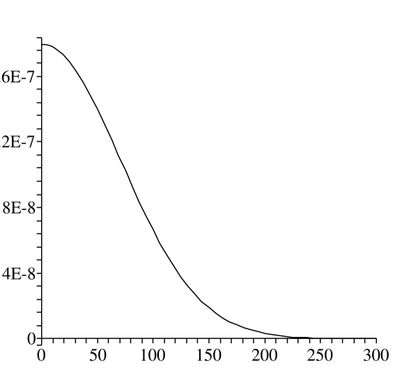
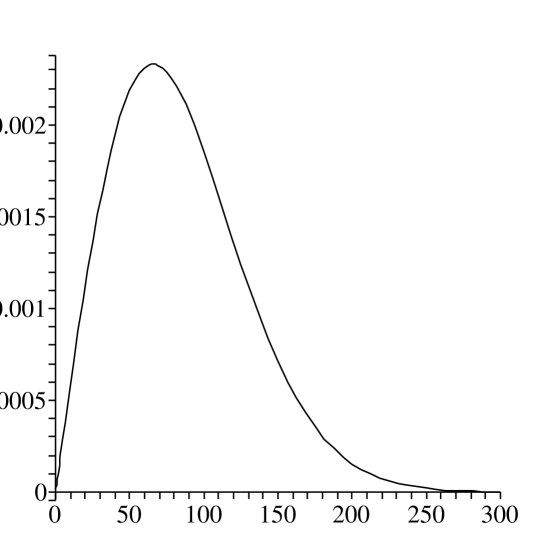
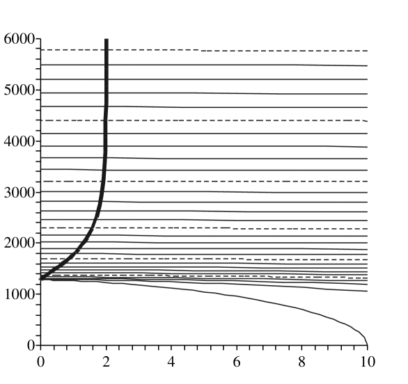
Figure 2: Collapse of a dust ball

We begin with the example of a non-uniform dust ball collapsing to form a black hole. The initial density distribution is taken to be radially Gaussian so that

$$\rho_{o}=\frac{m_{o}}{\pi^{3/2}r_{o}^{3}}e^{-r^{2}/r_{o}^{2}}\,.$$ (37)

In this expression $m_{o}$ is the total mass of the cloud as read from the corresponding mass function $m(r)$ (equation 14) and also corresponds to its ADM mass. The parameter $r_{o}$ determines how much the cloud is initially “spread out”. Such a distribution is pictured in figure 2a), where we have taken $r_{o}=100\,m_{o}$. $\rho$ is plotted in units of $m_{o}^{-2}$ and $r$ in units of $m_{o}$.

For this choice of parameters $r-2m(r)>0$ everywhere and so there are no marginally trapped surfaces in the initial time slice. Further, for any distribution of this kind condition (30) is met and therefore there are no shell crossings. In this case,

$$\tau_{c}(0)=\frac{\pi^{5/4}\sqrt{3}}{4\sqrt{2}}\sqrt{\frac{r_{o}^{3}}{m_{o}}}\approx 1281\,m_{o}\,,$$ (38)

and the first $r=\mbox{constant}$ shells collapse to zero area at that time. As this happens, the central density $\rho(\tau_{c},0)$ diverges to infinity (equation 20). Referring to 2c) we see that an MTT is born out of this divergence, while 2b) shows that it is everywhere spacelike and so is a dynamical horizon.

Note that in figure 2c) (as well as in future evolution graphs), the MTT is shown as the thick black line. The rest of the lines are $r=\mbox{constant}$ surfaces and correspond to the timelike geodesics that trace the evolution of individual dust shells. In this figure, most of them are very nearly horizontal as they have fallen in from a long way out and are moving very quickly (relative to the constant $\tau$ foliation) by the time that they approach the horizon.

Returning to the evolution graph 2c) we note that as $\tau\rightarrow\infty$, $R\rightarrow 2m_{o}$ and $C\rightarrow 0$ as the last bits of matter fall through the horizon and it asymptotes towards a null and isolated state.

Figure 3: Penrose-Carter diagram for dust-ball collapse. To obtain the full spacetime diagram, including the corresponding white hole and $\mathscr{I}^{-}$, reflect this diagram through the $\tau=\eta=0$ instant of time symmetry. Note that $r=0$ starts as a regular timelike geodesic in the centre of the ball and then changes into a spacelike singularity at $\tau=\tau_{c}(0)$ as the central density goes to infinity.

Many of these features of the evolution may also be seen in the Penrose-Carter diagram for the spacetime which is given in figure 3. Thus, we again see the MTT created out of the central spacelike singularity, evolving in a spacelike fashion, and finishing its evolution by asymptoting to the null event horizon. Note that for simplicity of presentation, this diagram shows a sharp cut-off of the dust distribution at some finite $r$. In our example this does not occur and instead the density asymptotes to zero. Thus, properly one should view the cut-off as as marking, say, the $r$ which contains $99.9\%$ of the mass. This diagram also nicely shows that while the MTT appears at the same time as the singularity, nothing in particular is happening at $r=0$ when the event horizon “appears”.

III.3.2 Smooth versions of Oppenheimer-Snyder collapse

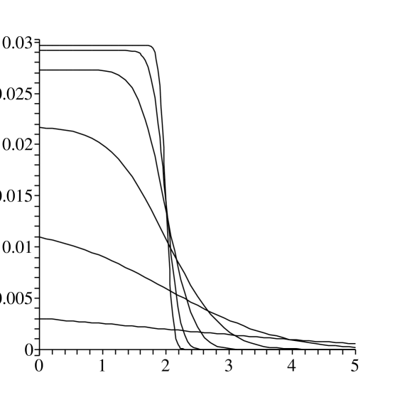
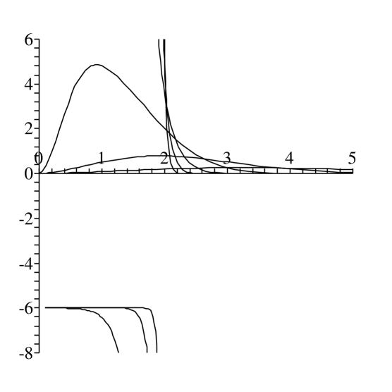
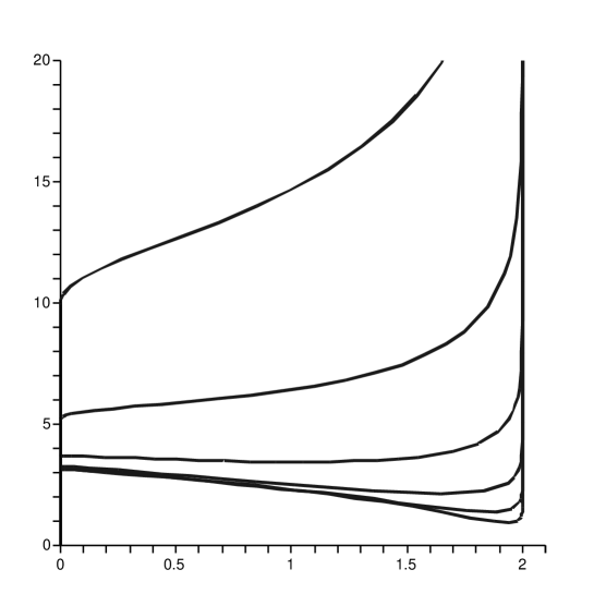
Figure 4: Approach to Oppenheimer-Snyder collapse

We now consider a family of spacetimes parametrized by a real number $\sigma$ where the initial density profiles are also not homogeneous but uniformly converge to a step function as $\sigma\rightarrow\infty$. These may then be viewed as interpolating between the collapse of a highly non-homogeneous dust ball like in the previous example, and Oppenheimer-Snyder collapse. As one would expect, in these examples we will encounter marginally trapped tubes that are partially spacelike and partially timelike.

In particular, consider initial densities of the form

$$\rho_{o}=\frac{m_{o}F(\sigma)}{r_{o}^{3}}\left(1-\mbox{erf}\left[\sigma\left(\frac{r}{r_{o}}-1\right)\right]\right)$$ (39)

where $F(\sigma)$ is a complicated function chosen so that $m_{o}=\lim_{r\rightarrow\infty}m(r)$ is the total dust mass, $r_{o}$ is the location on the “step” where $-d\rho/dr$ is a maximum, $\sigma$ characterizes the steepness of that step, and $\mbox{erf}(x)$ is the usual error function.

In the examples of Figure 4 we take $m_{o}$ as our length scale, choose $r_{o}=2m_{o}$, and consider a variety of values of $\sigma$. Then graph a) shows how the initial densities converge towards a step function with increasing $\sigma$. In the meantime graph b) shows that for smaller values of $\sigma$ the expansion parameter $C$ is always positive, while for the larger values it starts out negative with $C\approx-6$ while the density is approximately constant. This corresponds to the expected value of $C$ in the corresponding OS spacetime. It then diverges to $-\infty$, switches to being positive around $r=2m_{o}$ (when the main part of the step has fallen through), and then asymptotes to $0$ as the density of dust falling through the horizon also goes to zero. As expected, the switch in sign corresponds to the corresponding switch of ${\cal L}_{n}\theta_{(\ell)}$ — that is when the MTT becomes instantaneously tangent to $n^{a}$.

In c) we also see that in all cases a dynamical horizon asymptotes to $R=2m_{o}$ as the last bits of dust fall through it. However, the MTT behaviour before that time varies greatly. For small values of $\sigma$ it continuously increases in area. For large values, we see that there are both increasing and decreasing regions. Somewhat confusingly it appears that for $\sigma=2$ there are both increasing and decreasing regions as well, even though b) shows that $C>0$ everywhere. We will return to examples such as this in section III.5.1, but for now we just keep in mind that spacelike surfaces can intersect in non-trivial ways. Here the dynamical horizon is demonstrating this as it intersects some of the $\tau=\mbox{constant}$ surfaces twice. The possibility of such foliation effects was also noted in ams05 .

Note that the timelike membranes in this example all go to zero areal radius around $\tau=\pi m_{o}$. This is not surprising as for large values of $\sigma$, $\tau_{c}\approx\pi m_{o}$ (eq. (31)). Thus, the membranes vanish as the first dust shells also collapse to zero areal radius — that is they disappear into the density singularity.

Finally, note that the spacetime diagrams for these spacetimes would be very similar to that shown in figure 3. The only significant difference would be that for the spacetimes with timelike membranes, the MTT would emerge from/vanish into the singularity as a timelike rather than spacelike surface – the slope of the MTT would be greater than $45^{\circ}$.

III.4 Accretion onto a pre-existing hole

The next two examples study the accretion of dust shells onto a pre-existing black hole. In the first example a black hole will substantially increase its mass while the MTT remains null or spacelike everywhere through the evolution. In the second example we study a very large matter shell falling into a black hole; here we will again see timelike membranes.

III.4.1 Small dust shell falls into black hole

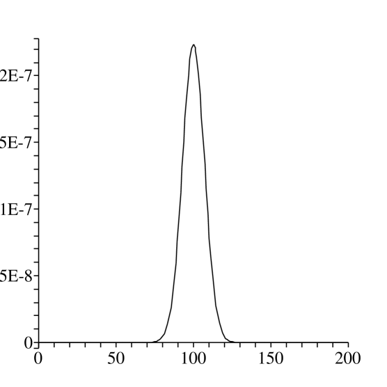
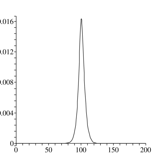
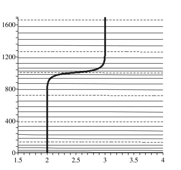
Figure 5: Small dust shell

We begin with a dust shell of the form

$$\rho_{o}=\frac{m_{o}e^{-\left(\frac{r}{r_{o}}-\alpha\right)^{2}}}{2\pi^{3/2}(1+2\alpha^{2})r_{o}^{3}}\,,$$ (40)

where $m_{o}$ measures the total mass of the shell (ie. the asymptotic behaviour of the associated mass function), $r_{o}$ characterizes its “thickness”, and $\alpha$ gives its initial position in terms of $r_{o}$. Again this distribution is Gaussian, but this time it is a shell with peak density at $\alpha r_{o}$. We wish to study the accretion of such a shell onto a pre-existing black hole and so excise a small region in the interior of the shell spacetime and replace it by a Schwarzschild geometry with mass parameter $M$, putting the junction at some $r=\hat{r}>2M$. From the discussion in subsection III.1, for $r>\hat{r}$ the mass function must then be $m(r)=M+4\pi\int_{\hat{r}}^{r}\rho_{o}(\bar{r})\bar{r}^{2}d\bar{r}$.

An example of such a spacetime is shown in Figure 5, where we have chosen $\hat{r}=2.5\,M$, $m_{o}=M/2$, $\alpha=10$, and $r_{o}=10\,M$. Note that the parameters cannot be chosen arbitrarily in this case as shell crossings can easily develop. In fact, a small increase of the mass parameter so that $m_{o}\approx 0.7\,M$ will be sufficient to cause these. That said, for the parameters that we have chosen this does not occur, and we see that the horizon is initially quiescent and begins to expand as the dust falls through it. The expansion is spacelike (from figureIIIb), $C>0$), peaks as the largest density of matter crosses the horizon, and then tails off along with the infalling dust. Asymptotically the horizon becomes null again with areal radius $R=3\,M$, so that the mass function tends to $m=\frac{3}{2}M$.

Figure 6: Partial Penrose-Carter diagram showing the accretion of a small dust shell onto a pre-existing black hole. To get the full diagram this one should be : 1) continued on its left side with the Schwarzschild solution corresponding the the initial mass and 2) reflected through the instant of time symmetry.

Figure 6 shows the corresponding spacetime diagram. From the spacetime surgery, inside the dust shell the spacetime is Schwarzschild with mass $M$. However, as the dust reaches and crosses the MTT, it begins to expand in a spacelike manner and continues to do so as long as the dust continues to fall in. Ultimately as that density goes to zero the MTT asymptotes to the null event horizon. As in figure 3 the MTT clearly reacts to physical events while the event horizon, being teleologically defined, does not. Note too that as in that earlier diagram, the dust distribution is again, for simplicity, shown with an edge.

III.4.2 Large shell of approximately constant density falls into black hole

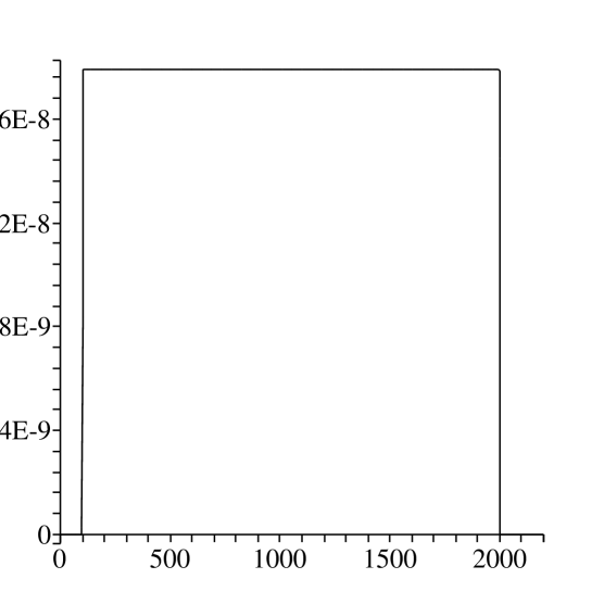
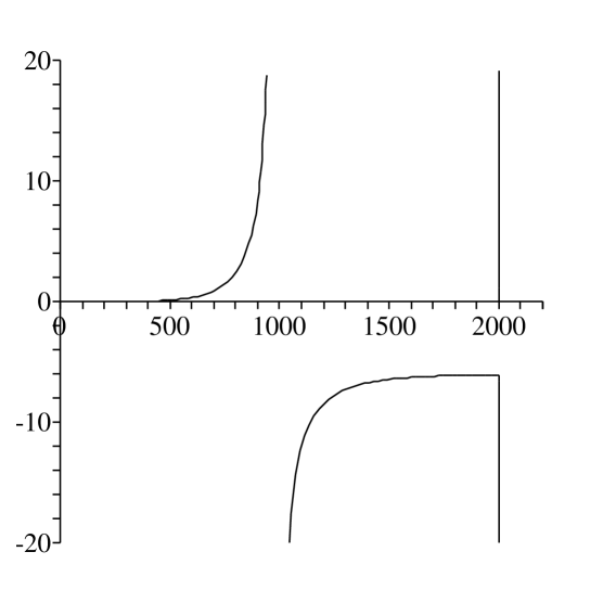
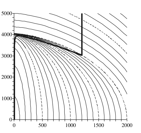
Figure 7: Large shell of constant density

In the previous example, the expansion was everywhere spacelike. It described a fairly dramatic situation, a significant expansion of a pre-existing black hole, however there was no sign of timelike membranes and the MTTs were isolated or dynamical horizons. We will now construct an example with timelike membranes. This will essentially be a smooth version of one of the more complicated Oppenheimer-Snyder examples presented in bendov04a . Thus, we build a spacetime in which a large amount of (initially) constant density dust falls into a black hole. The initial density is given by

$$\rho_{o}=\frac{3m_{o}\left(\mbox{erf}(\frac{r-r_{1}}{M})-\mbox{erf}(\frac{r-r_{2}}{M})\right)}{4\pi(r_{2}-r_{1})(2r_{1}^{2}+2r_{1}r_{2}+2r_{2}^{2}+3M^{2})}\,,$$ (41)

where $r_{1}$ and $r_{2}$ mark the (approximate) start and end of the shell, $m_{o}$ is the total mass of the shell as read from the mass function. Excision is performed and the interior is replaced by a black hole with mass $M$, which joins onto the dust exterior at some $r=\hat{r}>2M$. The full mass function for $r>\hat{r}$ will then be $m(r)=M+4\pi\int_{\hat{r}}^{r}\rho_{o}(\bar{r})\bar{r}^{2}d\bar{r}$.

For this example we choose $r_{1}=100\,M$, $r_{2}=2000\,M$, and $m_{o}=600\,M$. Thus, the mass of the hole will increase dramatically during the evolution from $m=M$ to $m=601\,M$. This evolution is shown in figure 7. Note that despite the appearance of the density function, it is actually smooth for $r>\hat{r}$ since the error functions themselves are smooth. Further, the density function will “spread” as it falls towards the hole and so the dust will not be of constant density as it crosses the horizon.

That said, we see that the horizon begins to expand in the usual way as the initial matter falls into it. Then however, something different happens. Considering evolution with respect to $\tau$ we see that around $\tau=3000\,M$, a new marginally trapped surface appears at $R=1202\,M$ and bifurcates into a dynamical horizon and a timelike membrane. The dynamical horizon quickly asymptotes to an isolated horizon while the timelike membrane contracts and eventually annihilates with the dynamical horizon that grows out to meet it.

Alternatively if we consider evolution with respect to the initial areal radius $r$, the MTT starts off almost-isolated, becomes dynamical as the first mass falls in, then goes null (with $-n^{a}$ as a tangent) and becomes a timelike membrane that continues to expand as it travels backwards in time. Finally, as the last dust falls through, it again goes null (with $-n^{a}$ as a tangent), dynamical, and then asymptotes back towards isolation.

The spacetime diagram for this evolution would be very similar to that shown in figure 6. The only difference would be that, during its active phase, the MTT would sometimes be timelike and so have a slope greater than $45^{\circ}$.

III.5 More complicated collapse

The previous examples display the basic behaviours of marginally trapped tubes — spacelike expansions, creation from singularities, and timelike contractions/backwards-in-time-expansions (depending how one views the evolution). In this section, to get a feel for the possible range of evolutions, we will consider examples generated from more complicated initial conditions that combine several of these behaviours.

III.5.1 Spacelike expansion/multiple horizons

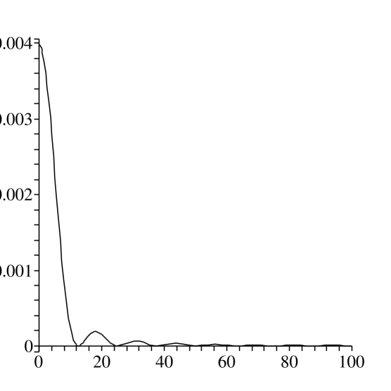
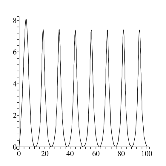
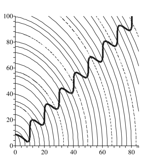
Figure 8: Multiple dust shells fall into a black hole

This example elaborates on a behaviour that we noted in section III.3.2. Namely it shows that the appearance of multiple horizons in a given leaf of a spacetime foliation does not always signal the existence of timelike membrane sections of the MTT. That is, a dynamical horizon as a spacelike surface can interweave with a foliation (of other spacelike surfaces) in highly non-trivial ways.

We will consider matter distributions of the form

$$\rho_{o}=\frac{\alpha\mu}{2\pi^{2}r_{o}r^{2}}\sin^{2}\left(\alpha\frac{r}{r_{o}}\right)\,,$$ (42)

where $r_{o}$ is an arbitrary reference length scale. When this is integrated to a mass function, we see that for any positive integer $N$ there is an amount of mass $\mu$ between $r=N\pi r_{o}/\alpha$ and $r=(N+1)\pi r_{o}/\alpha$. Thus, physically this corresponds to a series of shells each with the same mass (though decreasing density). Again one has to choose parameters with care to avoid shell crossings and/or initial black holes. A particular choice that meets these criteria is $\mu=(8\pi/5)\,r_{o}$ and $\alpha=1/4$. This is the distribution whose initial configuration and evolution is shown in figure 8.

Then, from Figure 8c), it is clear that $\tau=\mbox{constant}$ surfaces in this spacetime will contain either one or three marginally trapped surfaces (except at turning points of the MTT, where they contain two). Further, these will expand and contract in apparently the same kinds of ways that we have seen previous example which include timelike membranes. However, an examination of Figure 8b), shows that despite this behaviour, the expansion parameter $C$ is always greater than zero and so the MTT is everywhere either spacelike or null/isolated. Then the apparent contractions/expansions arise simply because the MTT intersects the foliation in non-trivial ways.

In Figure 8c), the horizon goes vertical/null at intervals of $R=2\mu\approx 10\,r_{o}$. Each of these corresponds to the density going to zero between each shell of mass $\mu=(8\pi/5)\,r_{o}\approx 5\,r_{o}$ and so the horizon becoming instantaneously isolated. Finally, note that with a careful choice of the parameters, the newly created MTT can absorb shells of this type for arbitrarily long periods of time, always alternating between being dynamical and isolated. Thus, a horizon can absorb an arbitrarily large amount of mass without ever going timelike. It is the rate of absorption, not the total amount that is significant in this regard.

III.5.2 Multiple timelike membranes

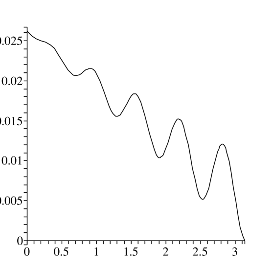
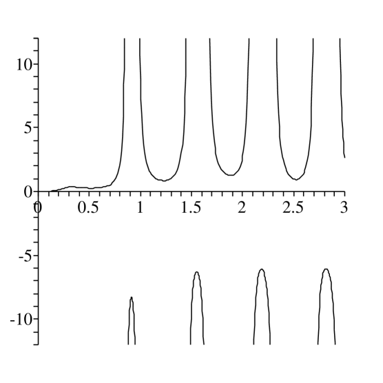
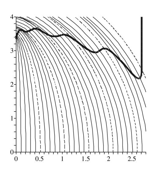
Figure 9: A more complicated dust collapse.

Our final example will demonstrate a spacetime that contains a MTT made up of multiple dynamical horizon and timelike membrane regions. The dust density will take the form:

$$\rho_{0}=\left\{\begin{array}[]{ll}\frac{\alpha}{r_{o}^{2}}\left[\pi-\frac{1}{5}\frac{r}{r_{o}}\left(3+2\cos^{2}\left(5\frac{r}{r_{o}}\right)\right)\right]&0\leq r\leq\pi r_{o}\\ \\ 0&r>\pi r_{o}\end{array}\right.$$ (43)

where $\alpha$ is a dimensionless constant. The exterior of $\pi r_{o}$ was excised to avoid negative density dust and so violations of the energy conditions. Thus, outside of that radius, the geometry will be Schwarzschild with mass $M=m(\pi r_{o})$.

Taking $\alpha=1/120$ there are neither shell-crossings nor initial black holes in this spacetime. The evolution is then shown in the graphs of figure 9. The initial density is irregular and gives rise to an MTT which, if we think of evolution as parameterized by $r$, starts out as a dynamical horizon and then alternates back and forth between being timelike and spacelike with (non-isolated) null cross-sections separating these regions. From the point of view of evolution with respect to $\tau$, spacelike slices have anywhere between one and five marginally trapped surfaces in this example. However, all of these intricacies are contained within the outermost isolated horizon (and here it really is isolated since we cut the density distribution at $r=\pi r_{o})$ and would not be visible to outside observers.

IV Scalar fields

In the previous section we have seen that the potential MTT behaviours suggested by (7) and (8) are all achieved by the dust spacetimes. Thus, depending on the initial configuration, the MTT can be any of spacelike, null, or timelike. In this section we will attempt the same demonstration for the scalar fields. Thus, we will consider initial configurations of scalar fields, evolve them in time, and examine the behaviour of any MTT that forms with the help of the expansion parameter $C$.

Given that scalar fields are significantly more complicated than dust we will necessarily take a numerical rather than an analytic approach. Section IV.1 will introduce the numerical model and the subsequent sections will present the results for two different scalar fields configurations. These will be analogous to configurations considered in the last section. The first, in section IV.2, examines the evolution of a initially smooth step-like configuration that collapses to form a black hole. The second, in section IV.3, studies a shell of scalar field which falls into an existing black hole. Due to numerical complexities, these results will be less complete than those considered in the last section, but will still demonstrate some interesting and complementary behaviours.

IV.1 Numerical approach

We will be interested in the scalar fields briefly considered in section II.2.3. The equations governing spacetimes containing these fields are generated by the Lagrangian:

$${\cal L}=\sqrt{-g}\left[\frac{1}{16\pi}R-\frac{1}{2}\nabla_{\alpha}\phi\nabla^{\alpha}\phi-V(\phi)\right]\;.$$ (44)

This class of models includes the massive Klein-Gordon field with $V=m_{0}\phi^{2}/2$ and in the following we will restrict ourselves to this case.

To solve the resulting coupled Einstein-Klein-Gordon equations we work with the standard 3+1 approach based on the ADM equations ADM and in particular adopt the techniques introduced in Regular to perform the evolutions. Restricting to spherical symmetry, we can then study the general evolutions by considering the dynamics of spacetimes with metrics of the form

$$ds^{2}=-\alpha^{2}(r,t)dt^{2}+A(t,r)dr^{2}+r^{2}B(r,t)\left(d\theta^{2}+\sin^{2}\theta d\varphi^{2}\right)\;.$$ (45)

The spherical symmetry implies that all dynamical functions depend only on $r$ and $t$. $\alpha$ is the usual lapse function and for simplicity we impose a vanishing-shift gauge condition; equivalently the “time-evolution” vector, $\partial/\partial t$ is everywhere orthogonal to the $t=\mbox{constant}$ “instantaneous” three-surfaces.

Focusing on this natural foliation with respect to $t$, we note that these hypersurfaces have intrinsic three-metric and extrinsic curvature :

$$h_{ab} = A[dr]_{a}[dr]_{b}+Br^{2}\Omega_{ab}\;\;\mbox{and}$$ (46)

$$K_{ab} = \frac{1}{2\alpha}\left(\frac{\partial A}{\partial t}\right)[dr]_{a}[dr]_{b}+\frac{1}{2\alpha}\left(\frac{\partial B}{\partial t}\right)\Omega_{ab}\,,$$ (47)

respectively, where $\Omega_{ab}$ was defined following equation (17). These, together with the value of the scalar field, are the variables whose evolution we will study.

Then, in the usual way we can rewrite the Einstein-Klein-Gordon equations in terms of the Hamiltonian and momentum constraints which restrict initial values of these quantities, in addition to evolution equations (which preserve the constraints). The actual implementation consists of picking an initial configuration for the scalar field, solving the constraints for $h_{ab}$ and $K_{ab}$ and finally using the evolution equation to obtain the dynamics of the corresponding spacetime. For brevity we will not include all of the details here; the interested reader is directed to Regular for a more detailed discussion.

Once we have a spacetime evolution, the next step is to search for an MTT. In this case it is natural to search for apparent horizons/marginally trapped surfaces within the $t=\mbox{constant}$ slices and this is what we will do. Since we are in spherical symmetry we need only consider the null expansions of the $r=\mbox{constant}$ two-surfaces. Then, with

$$u_{a}=-\alpha[dt]_{a}\;\;\mbox{ and }\;\;s_{a}=\sqrt{A}[dr]_{a}\,,$$ (48)

as the forward-in-time and towards-infinity pointing unit normals to the two-surfaces, we define

$$\ell_{a}=u_{a}+s_{a}\;\;\mbox{ and }\;\;n_{a}=\frac{1}{2}(u_{a}-s_{a})$$ (49)

as the outward and inward forward-in-time pointing null normals to those same surfaces. As in the dust examples, the exact “normalization” is irrelevant as we are only interested in the signs of the ensuing quantities, not their magnitudes. Thus, we can make this specific, convenient, choice. Then, it is straightforward to see that:

$$\theta_{(\ell)} = {\cal D}_{a}s^{a}+K-K_{ab}s^{a}s^{b}=\frac{\partial_{t}B}{\alpha B}+\frac{1}{A^{1/2}}\left(\frac{2}{r}+\frac{\partial_{r}B}{B}\right)$$ (50)

$$\theta_{(n)} = -\frac{1}{2}({\cal D}_{a}s^{a}-K+K_{ab}s^{a}s^{b})=\frac{\partial_{t}B}{2\alpha B}-\frac{1}{2A^{1/2}}\left(\frac{2}{r}+\frac{\partial_{r}B}{B}\right)\,,$$ (51)

where ${\cal D}_{a}$ is the covariant derivative compatible with $h_{ab}$ and $K=h^{ab}K_{ab}$ (as a quick check that these expressions are reasonable, note that for Minkowski space where $A=B=1$, $\theta_{(\ell)}=2/r>0$ and $\theta_{(n)}=-1/r<0$). In the code we evaluate these expressions over the whole numerical grid and look for places where $\theta_{(\ell)}$ changes signs and $\theta_{(n)}<0$. The corresponding two-spheres are then identified as the marginally trapped two-spheres which foliate the MTTs, and their area is

$$A_{AH}=4\pi r_{AH}^{2}B_{AH}\;$$ (52)

where $B_{AH}$ is the metric function $B$ evaluated at $r=r_{AH}$, the coordinate radius of these two-spheres.

Finally, the expansion parameter $C$ for this surface can be calculated using (13).

IV.2 Scalar field “step” collapses to form a black hole

Our first example will be analogous to the dust ball collapses considered in section III.3. As for those dust examples, our initial slice will be a moment of time symmetry ($K_{ab}=0$) and further we will choose our coordinates so that the coordinate radius $r$ will also be the areal radius $R$ on that slice (thus $B=1$ initially). Then, we specify a step-like configuration of the scalar field as shown in figure 10a).

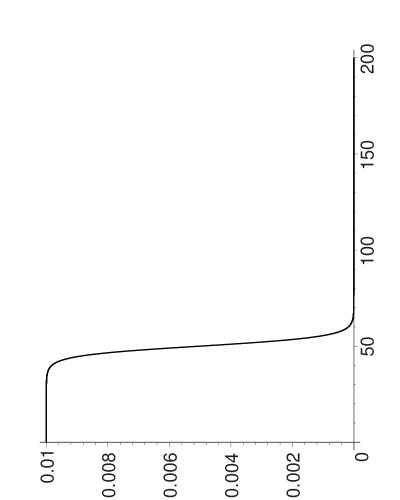
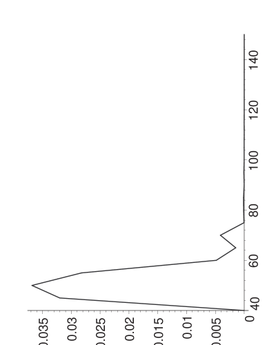
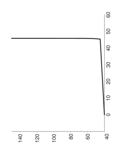
Figure 10: Scalar field “step”

Solving the constraint equations to find the initial form of $A$, we can then integrate the data as discussed above to find how the geometry and fields evolve in time. The results are shown in figures 10b) and 10c). The first thing to note is that throughout this collapse $C>0$ and so the MTT is a dynamical horizon. Secondly, as in the earlier examples it asymptotes to null as the spacetime settles down to become Schwarzschild. Note from figure 10c) that initially the hypersurfaces do not contain an apparent horizon. However, during the collapse an apparent horizon appears and then keeps growing until it reaches a constant size.

IV.3 Scalar field “shell” accretes onto existing black hole

Our second scalar field example is analogous to the dust shell examples of section III.4. Thus we will consider an initial “shell” of scalar field that accretes onto an existing black hole of mass $M$. After surgically inserting the black hole we again start out on a slice of time symmetry, though in this case for technical reasons do not start with $r$ as the areal radius. Instead, on the initial slice $\tilde{B}=1$, where $B=\left(1+\frac{M}{2r}\right)^{4}\tilde{B}$.

Then, as our initial scalar field conditions we consider a $\phi(0,r)$ of the form shown in figure 11a). The corresponding initial intrinsic geometry (essentially only $A$ remains unknown) is then found by solving the constraint equations. The results for the corresponding evolution are then shown in figures 11b) and 11c). On those graphs we again see that $C$ remains everywhere non-negative and asymptotes to zero at late times. Note too the apparent horizon on the initial hypersurface which grows as the scalar field falls into the hole.

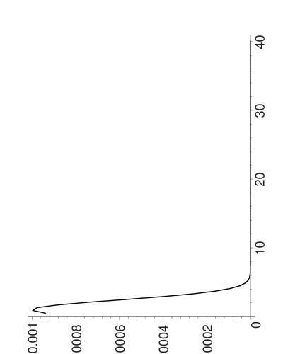
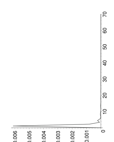
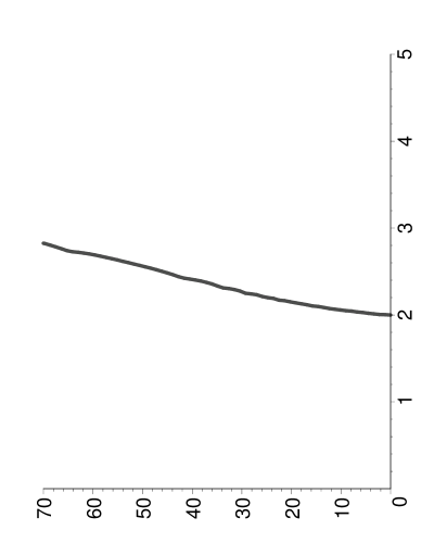
Figure 11: Scalar field accretion

IV.4 Outlook for scalar fields

Neither of the preceding examples included timelike membrane regions of the MTT. We believe that this is a reflection of the examples that our code has been able to integrate rather than a fundamental result. From (13) it is clear that a timelike membrane will only appear in situations where there is a sufficiently large concentration of the scalar field relative to the (inverse) area of the horizon. Our code had difficulty evolving such examples and so the lack of timelike membranes is not especially surprising. Physically, one would also expect it to be more difficult to obtain such examples for a massive scalar field which, in contrast to pressureless dust, resists compression. We expect that future investigations will find the appropriate combination of initial conditions needed to generate examples of timelike membranes in scalar field spacetimes. For now though, we simply note that our examples show timelike evolutions are not the rule for scalar field spacetimes.

V Conclusions and Speculations

In this paper we have seen that dynamical horizons and timelike membranes characterize two possible modes of black hole expansion. In the first a black hole/MTT smoothly expands as matter falls into it. By contrast, the second occurs when matter densities are high enough to force the formation of a new horizon of non-zero area that encloses any already existing MTTs.

Further insight into these two possibilities can be gained by considering the magnitudes of the quantities involved. As seen in the discussion of II, assuming that the null energy condition holds, the signature of an MTT is determined by the relative magnitudes of $1/A$ and $2T_{ab}\ell^{a}n^{b}$, or, specializing to (pressureless) dust, $1/A$ and $\rho$. Converting into physical units, it is straightforward to see that for a Schwarzschild black hole of mass $M=\mu M_{\odot}$, the inverse horizon area corresponds to a density

$$\rho_{A}=\frac{c^{6}}{16\pi G^{3}M_{\odot}^{2}}\frac{1}{\mu^{2}}\,,$$ (53)

where $M_{\odot}=2\times 10^{33}$ g is the approximate mass of the Sun and $c$ and $G$ are respectively the speed of light and the gravitational constant. Then, for a solar mass black hole, $\rho_{A}\approx 10^{16}\,\,\mbox{g}/\mbox{cm}^{3}$ which is about an order of magnitude higher than the density of a neutron star. By contrast, for a supermassive black hole of mass $10^{8}\,M_{\odot}$, one has $\rho_{A}\approx 1\,\,\mbox{g}/\mbox{cm}^{3}$, the density of water.

Though strictly speaking these results only apply in situations of spherical symmetry, it seems fairly safe to use them to draw some more general conclusions. Specifically, it is likely that both modes of expansion are not only mathematically possible as we have seen in this paper, but also both occur in physical situations. For small black holes, even if the lack of spherical symmetry changes these estimates by several orders of magnitude, it appears that dynamical horizon spacelike expansions are probably the dominant mode in all but the most extreme situations, such as black hole and/or neutron star collisions. Numerical studies support this contention as in such extreme situations the occurrence of multiple horizons appears to be generic num3 ; badridavid (though also relatively unstudied in a systematic way, since in most studies it is the exterior spacetime that is of interest and so the interior of the outermost apparent horizon is excised and thrown away). By contrast for supermassive black holes, it is likely that horizon jumps/TLMs are much more common.

These examples also suggest other (possible) properties of MTTs. First, dynamical horizons appear to only originate either out of singularities (the density singularities of III.3) or as part of a dynamical horizon/TLM pair (as in III.5.2). Equivalently, in all of our examples there is just one MTT associated with each black hole. This originates in a singularity and then weaves backwards and forwards in time, always expanding in area (relative to a foliation parameter that monotonically increases as one moves away from the singularity). This suggests that a similar result may be true away from spherical symmetry — the multiple horizons/jumps seen in numerical studies of black hole collisions may actually all be part of a single MTT that weaves backwards and forwards in time.

In our examples it is also true that TLMs and dynamical horizons always occur in such a way that a causal signal originating from the MTT would never be detectable by sufficiently far-away observers. This is consistent with a gravitational confinement theorem due to Israel israel1 ; israel2 which states that if the weak energy condition holds (as is the case in all our examples), a trapped two-sphere can be extended to a spacelike three-cylinder foliated by trapped two-spheres of constant area. Assuming reasonably regular spacetimes, this three-cylinder will act as a permanent one-way membrane for causal effects. Even though an observer “inside” an MTT can escape that trapped region, he will not be able to send signals beyond the areal radius of the two-sphere on which the MTT was first crossed. We note that Israel’s confinement theorem is quite general; it does not assume spherical symmetry or even asymptotic flatness. Moreover, in appropriate asymptotically flat spacetimes, trapped surfaces must necessarily be contained within event horizons and so unable to send causal signals to null infinity hawkingellis72 ; wald . Our asymptotically flat examples are also consistent with the latter: the outermost parts of MTTs are dynamical horizons which asymptote to a null surface with some finite area. Consequently, in physically realistic spacetimes, any TLMs that may be present will be hidden from observers far from a black hole, also in the absence of spherical symmetry.

In summary, even though the examples and (dust) calculations that we have seen in this paper are quite simple we believe that they are extremely useful in forming a correct intuition about the behaviour of MTTs during general black hole evolution. In particular they provide a convenient testing ground for ideas about these evolutions which is much simpler than full numerical simulations of black hole collisions and yet still significantly richer (and more realistic) than the heretofore studied analytical examples (Vaidya and Oppenheimer-Snyder). As such they should be useful in, among other things, suggesting possible extensions of the recent mathematical investigations abhaygreg ; ams05 of MTT properties.

References

- (1) S.W. Hawking and G.F.R. Ellis, The large scale structure of space-time (Cambridge University Press, Cambridge, 1972)
- (2) R.W. Wald, General Relativity (University of Chicago Press, Chicago, 1984)
- (3) W. Collins, Mechanics of apparent horizons, Phys. Rev. D45 495-498, 1992
- (4) S.A. Hayward, General laws of black-hole dynamics, Phys. Rev. D49 6467–6474, 1994
- (5) S.A. Hayward, Gravitational waves from quasispherical black holes, Phys.Rev. D61 101503, 2000
- (6) S.A. Hayward, Gravitational radiation from dynamical black holes, gr-qc/0505050, 2005
-
(7)
A. Ashtekar, C. Beetle and S. Fairhurst,
Isolated horizons: a generalization of black hole mechanics,
Class. Quantum Grav. 16 L1–L7, 1999;
A. Ashtekar, A. Corichi and K. Krasnov, Isolated horizons: the classical phase space, Adv. Theor. Math. Phys. 3 419–478, 2000;
A. Ashtekar, C. Beetle and S. Fairhurst, Mechanics of isolated horizons, Class. Quantum Grav. 17 253–298, 2000;
A. Ashtekar, A. Corichi, Laws governing isolated horizons: inclusion of dilatonic couplings, Class. Quantum Grav. 17 1317–1332, 2000;
A. Ashtekar, S. Fairhurst and B. Krishnan, Isolated horizons: Hamiltonian evolution and the first law, Phys. Rev. D62 104025, 2000;
A. Ashtekar, C. Beetle, O. Dreyer, S. Fairhurst, B. Krishnan, J. Lewandowski and J. Wiśniewski, Generic isolated horizons and their applications, Phys. Rev. Lett. 85 3564–3567, 2000;
A. Ashtekar, C. Beetle and J. Lewandowski, Mechanics of rotating isolated horizons, Phys. Rev. D64 044016, 2001 - (8) A. Ashtekar, C. Beetle and J. Lewandowski, Geometry of generic isolated horizons, Class. Quantum Grav. 19 1195–1225, 2002
-
(9)
A. Ashtekar, J. Baez and K. Krasnov, Quantum geometry of isolated
horizons and black hole entropy, Adv. Theor. Math. Phys.
4 1–94, 2000;
A. Ashtekar, J. Engle and C. Van Den Broeck, Quantum horizons and black hole entropy: Inclusion of distortion and rotation, Class. Quantum Grav. 22 L27–L34, 2005 - (10) A. Ashtekar and B. Krishnan, Dynamical horizons: energy, angular momentum, fluxes and balance laws, Phys. Rev. Lett. 89 261101, 2002
- (11) A. Ashtekar and B. Krishnan, Dynamical horizons and their properties, Phys. Rev. D68 104030, 2003
-
(12)
S.A. Hayward,
Energy conservation for dynamical black holes,
Phys. Rev. Lett. 93 251101, 2004;
S.A. Hayward, Energy and entropy conservation for dynamical black holes, Phys. Rev. D70 104027, 2004 - (13) I. Booth and S. Fairhurst, Horizon energy and angular momentum from a Hamiltonian perspective, Class. Quantum Grav 22 4515-4550, 2005
- (14) H. Shinkai and S. Hayward, Quasi-spherical approximation for rotating black holes, Phys.Rev. D64 044002, 2001
- (15) I. Booth and S. Fairhurst, The first law for slowly evolving horizons, Phys. Rev. Lett. 92 011102, 2004
-
(16)
A. Ashtekar, J. Engle, T. Pawlowski and
C. Van Den Broeck,
Multipole moments of isolated horizons,
Class. Quantum Grav. 21 2549–2570, 2004;
C. Van Den Broeck, Ph.D. thesis, Penn State University, 2005 - (17) A. Ashtekar and G.J. Galloway, Some uniqueness results for dynamical horizons, Preprint gr-qc/0503109, 2005 (to appear in Advances in Theoretical and Mathematical Physics)
- (18) L. Andersson, M. Mars, and W. Simon, Local existence of dynamical and trapping horizons, Phys. Rev. Lett. 95 111102, 2005
- (19) O. Dreyer, B. Krishnan, E. Schnetter and D. Shoemaker, Introduction of isolated horizons in numerical relativity, Phys.Rev. D67 024018, 2003
- (20) L. Baiotti, I. Hawke, P.J. Montero, F. Löffler, L. Rezzolla, N. Stergioulas, J.A. Font, and E. Seidel, Three-dimensional relativistic simulations of rotating neutron star collapse to a black hole, Phys.Rev. D71 024035, 2005
- (21) E. Schnetter, F. Hermann, and D. Poulney, Horizon pretracking, Phys. Rev. D71 044033, 2005
- (22) S.A. Hayward, Black holes: new horizons, gr-qc/0008071, 2000
- (23) I. Ben-Dov, The Penrose inequality and apparent horizons, Phys. Rev. D70 124031, 2004
- (24) J.M.M. Senovilla, On the existence of horizons in spacetimes with vanishing curvature invariants, JHEP 0331 046, 2003
- (25) J.R. Oppenheimer and H. Snyder, On continued gravitational contraction, Phys. Rev. 56 455–459, 1939
- (26) J. Stewart, Advanced General Relativity (Cambridge University Press, Cambridge, 2003)
- (27) S. Chandrasekhar, The Mathematical Theory of Black Holes (Clarendon Press, Oxford, 2000)
- (28) J.M.M. Senovilla, Singularity theorems and their consequences, Gen. Rel. Grav. 30 701–848, 1998
- (29) W. Israel, The formation of black holes in nonspherical collapse and cosmic censorship, Can. J. Phys. 64 120–127, 1986
- (30) S.M.C.V. Gonçalves, Shell crossing in generalized Tolman-Bondi spacetimes, Phys.Rev. D63 124017, 2001
- (31) I. Booth, Black hole boundaries, gr-qc/0508107, 2005 (to appear in Can. J. Phys.)
- (32) V. Husain, E.A. Martinez, D. Nunez, Exact solution for scalar field collapse, Phys. Rev. D50 3783–3786, 1994
-
(33)
R. Arnowitt, S. Deser and C. W. Misner,
Gravitation: an introduction to current research,
in The dynamics of general relativity,
John Wiley and Sons, San Francisco, 1962;
J. York, Kinematics and dynamics of general relativity, Sources of Gravitational Radiation (Cambridge University Press, Cambridge, 1979) -
(34)
M. Alcubierre and J.A. Gonzalez,
Regularization of spherically symmetric evolution codes in numerical
relativity,
Comp. Phys. Comm. 167 76–84, 2005;
M. Alcubierre, J.A. Gonzalez and M.Salgado, Dynamical evolution of unstable self-gravitating scalar solitons, Phys. Rev. D70 064016, 2004 -
(35)
Private communication, Badri Krishan (2005).
Private communication, David Hobill (2005). - (36) W. Israel, Must nonspherical collapse produce black holes? A gravitational confinement theorem, Phys. Rev. Lett. 56 789–791, 1986