Wide parameter search for isolated pulsars using the Hough transform

Abstract

We use the Hough transform to analyze data from the second science run of the LIGO interferometers, to look for gravitational waves from isolated pulsars. We search over the whole sky and over a large range of frequencies and spin-down parameters. Our search method is based on the Hough transform, which is a semi-coherent, computationally efficient, and robust pattern recognition technique. We also present a validation of the search pipeline using hardware signal injections.

1 Introduction

This paper presents some partial results for a wide parameter space search for periodic gravitational waves using data from the LIGO detectors. The most promising sources for such waves are isolated pulsars. Previous searches for gravitational waves from pulsars have been of two kinds. The first is a search targeting pulsars whose parameters are known through radio observations. These searches typically use matched filtering techniques and are not very computationally expensive. An example of such a search is [1] which targets PSR J1939+2134 using data from the first science runs of the LIGO and GEO detectors. The end result is an upper limit on the strength of the gravitational wave emitted by this pulsar and therefore on its ellipticity. See also [2] which applies some of the techniques presented in [1] to a large number of known pulsars using data from the second science run of the LIGO detectors. The second kind of searches look for pulsars which have not yet been observed by radio telescopes. This involves searching over large parameter space volumes and turns out to be computationally limited. This is because looking for weak continuous wave signals requires large observation times to build up signal to noise ratio and to claim a detection with some degree of confidence; on the other hand, the number of templates that must be searched over, and therefore the computational requirements, increase rapidly with the observation time. An example of such a search is [3] where a 2-day long data stretch from the Explorer bar detector is used to perform an all sky search in a narrow frequency band around the resonant frequency of the detector.

All the searches mentioned above rely on a coherent integration over the full observation time; it is well known that this is the optimal method. However, a full coherent integration is computationally expensive and it is therefore also useful to consider methods which are less sensitive but computationally inexpensive. Such methods typically involve semi-coherent combinations of the signal power in short stretches of data. The Hough transform is an example of such a method [4]. Using this method, we perform an all-sky search over a large frequency range using two months of data from the LIGO detectors. As in all the searches mentioned above, we assume that the pulsar does not glitch during the full observation time considered.

Section 2 briefly describes the waveforms that we are looking for. Section 3 describes our search method, the Hough transform. The search pipeline and the parameter space we search over is given in section 4. The search results are given in section 5. Section 6 presents a validation of our search method using hardware injected signals and finally section 7 concludes with a summary of our results and plans for further work.

2 The expected waveform

The form of the gravitational wave emitted by an isolated pulsar, as seen by a gravitational wave detector is [5]:

$$h(t)=F_{+}(t,\psi)h_{+}(t)+F_{\times}(t,\psi)h_{\times}(t)$$ (1)

where $t$ is time in the detector frame, $\psi$ is the polarization angle of the wave, $F_{+,\times}$ are the detector antenna pattern functions for the two polarizations. If we assume the emission mechanism is due to deviations of the pulsar’s shape from perfect axial symmetry, then the gravitational waves are emitted at a frequency which is twice the rotational rate $f_{r}$ of the pulsar. Under this assumption, the waveforms for the two polarizations $h_{+,\times}$ are given by:

$$h_{+}=h_{0}\frac{1+\cos^{2}\iota}{2}\cos\Phi(t)\,,\qquad h_{\times}=h_{0}\cos\iota\sin\Phi(t)\,,$$ (2)

where $\iota$ is the angle between the pulsar’s spin axis and the direction of propagation of the waves, and $h_{0}$ is the amplitude:

$$h_{0}=\frac{16\pi^{2}G}{c^{4}}\frac{I_{zz}\epsilon f_{r}^{2}}{d}\,.$$ (3)

Here $d$ is the distance of the star from Earth, $I_{zz}$ is the $z$-$z$ component of the star’s moment of inertia with the $z$-axis being its spin axis, and $\epsilon$ is the equatorial ellipticity of the star. The phase $\Phi(t)$ takes its simplest form in the Solar System Barycenter (SSB) frame where it can be expanded in a Taylor series. Up to second order:

$$\Phi(t)=\Phi_{0}+2\pi\left(f_{0}(T-T_{0})+\frac{1}{2}\dot{f}(T-T_{0})^{2}\right)\,.$$ (4)

Here $T$ is time in the SSB frame and $T_{0}$ is a fiducial start time. The frequency $f_{0}$ and the spin-down parameter $\dot{f}$ are defined at this fiducial start time. In this paper, we include only one spin-down parameter in our search, i.e. we ignore the higher order terms in Eq. (4). This is reasonable because, as we shall see below in section 4, our frequency resolution is too coarse for the higher spindowns to have any effect for reasonable values of the pulsar spindown age.

Neglecting relativistic effects which do not affect us significantly in this case (again because of the coarseness of our frequency resolution), the instantaneous frequency $f(t)$ of the wave as observed by the detector is given, to a very good approximation, by the familiar non-relativistic Doppler formula:

$$f(t)-\hat{f}(t)=\hat{f}(t)\frac{{\bf v}(t)\cdot\bf{n}}{c}$$ (5)

where $t$ is time in the detector frame, ${\bf v}(t)$ is the velocity of the detector at time $t$, $\bf{n}$ is the direction to the pulsar, $\hat{f}(t)$ is the instantaneous signal frequency at time $t$ and is given by

$$\hat{f}(t)=f_{0}+\dot{f}\left(t-t_{0}\right)\,.$$ (6)

Equations (5) and (6) describe the time-frequency pattern produced by a signal, and this is the pattern that the Hough transform is used to look for.

3 The Hough transform

The Hough transform was invented by Paul Hough in 1959 as a method for finding patterns in bubble chamber pictures from CERN [6] and it was later patented by IBM [7]. The Hough transform is also well known in the literature on pattern recognition to be a robust method for detecting straight lines, circles etc. in digital images; see e.g. [8] for a review in this field. A detailed discussion of the Hough transform as applied to the search for continuous gravitational waves can be found in [4]. A closely related semi-coherent method is the stack-slide algorithm described in [9].

The idea of the Hough transform can be illustrated by the following simple example. Consider the problem of trying to detect straight lines in a noisy two-dimensional digital image. The digital image is assumed to be made up of pixels which can be in one of only two possible states, namely “on” or “off”. Let $(x,y)$ be the coordinates of the center of a typical pixel. We are looking for a pattern which is parameterized by two numbers $(m,c)$ such that

$$y=mx+c\,.$$ (7)

The parameter space $(m,c)$ is assumed to be suitably digitized so that it is also made up of pixels. To find the most likely value of $(m,c)$, we proceed as follows. For each pixel $(\hat{x},\hat{y})$ which is “on”, we mark all the possible values of $(m,c)$ which are consistent with it, i.e. we mark all pixels in the $(m,c)$ plane lying on the straight line $\hat{y}=m\hat{x}+c$ with a “+1”. This is repeated for every pixel which is “on”. The end result is an integer, the number count, for every pixel in the $(m,c)$ plane. In the case when the digital image is too noisy and no straight lines can be detected, the number counts would be uniformly distributed in the $(m,c)$ place. The presence of a sufficiently strong signal would lead to a large number count in at least one of the $(m,c)$ pixels, and the largest number count would indicate the most likely parameter space values.

This method enables us to mark all the possible templates consistent with a given observation without stepping through the parameter space point-by-point. This leads to a significant gain in computational speed. Furthermore, each observation, no matter how noisy, only adds at the most $+1$ to the final number count. These two features are the chief virtues of the Hough transform method: computational speed and robustness. On the other hand, the Hough search is likely to be less sensitive than the stack-slide search considered in [9]. The tradeoffs between sensitivity versus efficiency and robustness are yet to be studied in detail and will be important in the context of a hierarchical search [9, 10].

In our case, the Hough transform is used to find a signal whose frequency evolution fits the pattern produced by the Doppler shift (5) and the spin-down (6) in the time-frequency plane. The parameters which determine this pattern are $(f_{0},\dot{f},\mathbf{n})$; a point in this four dimensional parameter space will be denoted by $\vec{\xi}$. This parameter space is covered by a discrete cubic grid whose resolution is described in section 4. The result of the Hough transform is a histogram, i.e. an integer (the number count) for each point of this grid. The starting point for the Hough transform are $N$ short stretches of Fourier transformed data; each short stretch will be called an SFT (Short Fourier Transform). Each of these SFTs is “digitized” by setting a threshold $\rho_{\textrm{\mbox{\tiny{th}}}}$ on the normalized power $\rho_{k}$ in the $k^{th}$ frequency bin:.

$$\rho_{k}=\frac{2|\tilde{x}_{k}|^{2}}{T_{\textrm{\mbox{\tiny{coh}}}}S_{n}(f_{k})}\,.$$ (8)

Here $\tilde{x}_{k}$ is the value of the Fourier transform in the $k^{th}$ frequency bin corresponding to a frequency $f_{k}$, $T_{\textrm{\mbox{\tiny{coh}}}}$ is the time baseline of the SFT, and $S_{n}(f_{k})$ is the single-sided power spectral density of the detector noise at the frequency $f_{k}$. We require that $T_{\textrm{\mbox{\tiny{coh}}}}$ is small enough so that the signal does not shift by more than, say, half a frequency bin within this time duration. For frequencies of $\sim 300$Hz, this restricts $T_{\textrm{\mbox{\tiny{coh}}}}$ to be lesser than $\sim 60$min [4]. In this paper, we work with SFTs for which $T_{\textrm{\mbox{\tiny{coh}}}}=1800$s. In principle, we could choose $T_{\textrm{\mbox{\tiny{coh}}}}$ to be greater, but we are restricted by the duty cycle of the interferometers in that we should be able to find suitably long time periods during which the detector is in lock. Furthermore, the data should be stationary over the chosen time period. The choice of $1800$s is a suitable compromise for all the three interferometers during the S2 run.

This thresholding produces a set of zeros and ones (called a “peakgram”) from each SFT. This set of peakgrams is the analog of the digitized two-dimensional image described earlier. The Hough transform is used to calculate the number count $n$ at each parameter space point starting from this collection of peakgrams. Let $p(n)$ be the probability distribution of $n$ in the absence of a signal, and $p(n|h)$ the distribution in the presence of a signal $h(t)$. It is clear that $0\leq n\leq N$, where $N$ is the number of SFTs, and it can be shown that for stationary Gaussian noise, $p(n)$ is a binomial distribution with mean $Nq$ where $q=e^{-\rho_{\textrm{\mbox{\tiny{th}}}}}$ is the probability that any frequency bin is selected:

$$p(n)=\left(\begin{array}[]{c}N\\ n\end{array}\right)q^{n}(1-q)^{N-n}\,.$$ (9)

In the presence of a signal, the distribution is ideally also a binomial but with a slightly larger mean $N\eta$ where, for weak signals, $\eta$ is given by

$$\eta=q\left\{1+\frac{\rho_{\textrm{\mbox{\tiny{th}}}}}{2}\lambda+\mathcal{O}(\lambda^{2})\right\}\,.$$ (10)

$\lambda$ is the signal to noise ratio within a single SFT, and for the case when there is no mismatch between the signal and the template:

$$\lambda=\frac{4|\tilde{h}(f_{k})|^{2}}{T_{\textrm{\mbox{\tiny{coh}}}}S_{n}(f_{k})}$$ (11)

with $\tilde{h}(f)$ being the Fourier transform of the signal $h(t)$ (see [4] for details). The approximation that the distribution in the presence of a signal is binomial breaks down for reasonably strong signals. This happens mainly due to two reasons: i) the random mismatch between the signal and the template used to calculate the number count and ii) the amplitude modulation of the signal which causes $\eta$ to vary from one SFT to another and for different sky locations. The result of these two effects is to “smear” out the binomial distribution in the presence of a signal.

Candidates in parameter space are selected by setting a threshold $n_{\textrm{\mbox{\tiny{th}}}}$ on the number count. The false alarm and false dismissal rates for this threshold are defined respectively in the usual way:

$$\alpha=\sum_{n=n_{\textrm{\mbox{\tiny{th}}}}}^{N}p(n)\,,\qquad\beta=\sum_{n=0}^{n_{\textrm{\mbox{\tiny{th}}}}-1}p(n|h)\,.$$ (12)

We choose the thresholds $(n_{\textrm{\mbox{\tiny{th}}}},\rho_{\textrm{\mbox{\tiny{th}}}})$ based on the Neyman-Pearson criterion of minimizing $\beta$ for a given value of $\alpha$. It can be shown [4] that this criterion leads, in the case of weak signals (i.e. $\lambda<<1$), large $N$, and Gaussian stationary noise, to $\rho_{\textrm{\mbox{\tiny{th}}}}\approx 1.6$. This corresponds $q=e^{-\rho_{\textrm{\mbox{\tiny{th}}}}}\approx 0.20$, i.e. we select about $20\%$ of the frequency bins from each SFT; for weak signals, this turns out to be independent of the choice of $\alpha$ and signal strength. Furthermore, $n_{\textrm{\mbox{\tiny{th}}}}$ is also independent of the signal strength and is given by:

$$n_{\textrm{\mbox{\tiny{th}}}}=Nq+\sqrt{2Nq(1-q)}\,\textrm{erfc}^{-1}(2\alpha)$$ (13)

where, as before, $q=e^{-\rho_{\textrm{\mbox{\tiny{th}}}}}$ and $\textrm{erfc}^{-1}$ is the inverse of the complementary error function. These values of the thresholds lead to a certain value of the false dismissal rate $\beta$ which is given in [4]. The value of $\beta$ of course depends on the signal strength, and it turns out that the weakest signal which will cross the above thresholds at a false alarm rate of $1\%$ and a false dismissal rate of $10\%$ is given by

$$h_{0}=\frac{8.54}{N^{1/4}}\sqrt{\frac{S_{n}(f_{0})}{T_{\textrm{\mbox{\tiny{coh}}}}}}$$ (14)

Equation (14) gives the smallest signal which can be detected by the search, and is therefore a measure of the sensitivity of the search.

The data analyzed in this paper correspond to LIGO’s second Science Run (S2) that was held for 59 days, from February 14 to April 14, 2003. The GEO detector was not running at that time, but all three LIGO detectors were operating with a significantly better sensitivity than during the first science run. The LIGO detectors comprise one 4 km facility in Livingston, Louisiana, (L1) and two, 4 km and 2 km respectively in Hanford, Washington (H1 and H2); see eg. [11]. For our purposes, we note that the duty cycles of the detectors during the S2 run were $37\%$ for L1, $74\%$ for H1 and $58\%$ for H2. The number $N$ of $30$min SFTs available for L1 data were 687, 1761 for H1 and 1384 for H2.

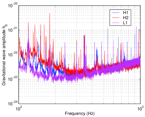
Figure 1: Typical sensitivities of the three LIGO detectors during the S2 run with a 1% false alarm rate and 10% false dismissal rate.

Figure 1 shows the expected sensitivity for the Hough search by the three LIGO interferometers during the S2 run. Those $h_{0}$ values correspond to the amplitudes detectable from a generic source with a 1% false alarm rate and 10% false dismissal rate, as given by Eq. (14). It should be kept in mind that Eq. (14) significantly over-estimates the sensitivity of the search for unknown pulsars because it does not include the mismatch between the signal and the template. Furthermore, due to the large number of templates involved in the search, a false alarm rate of $1\%$ is too large in practice, and it would result in too many potential candidates. A false alarm rate of $\sim 10^{-13}$ would be more realistic since this would lead, in the ideal case, to less than one candidate over the parameter space points considered in this search.

Assuming that the gravitational wave emission mechanism is due to deviations of the pulsar’s shape from perfect axial symmetry, from Eq. (3). (Eq. (2.9) in [4]) and Eq. (14), we can estimate the nominal astrophysical reach of the search for the three detectors:

$$d=\frac{16\pi^{2}GN^{1/4}I_{zz}\epsilon f_{r}^{2}}{8.54c^{4}}\sqrt{\frac{T_{\textrm{\mbox{\tiny{coh}}}}}{S_{n}(2f_{r})}}\,.$$ (15)

For a value of $I_{zz}=10^{45}\,\textrm{g-cm}^{2}$, $\epsilon=10^{-5}$, and for typical parameters of the S2 run, this corresponds to a distance of about $20$-$30$ parsecs. It should be kept in mind that this is not a realistic figure for the astrophysical reach of the search; it does not consider the mismatch between the template and signal, and it does not use the more realistic false alarm rate mentioned above. Due to these effects, it turns out that Eq. (15) overestimates the astrophysical reach by a factor of about $2$-$3$.

4 The search pipeline

Data from each of the three LIGO interferometers are used to analyze the same parameter space region. This section describes the portion of the parameter space $(f_{0},\dot{f},\mathbf{n})$ that we search over, and the resolution of our grid in this portion of the parameter space.

The total observation time is approximately $T_{\textrm{\mbox{\tiny{obs}}}}\approx 5.2\times 10^{6}$sec corresponding to the S2 science run. We search for pulsar signals in the frequency range $200$-$400$Hz with a frequency resolution: $\delta f={T_{\textrm{\mbox{\tiny{coh}}}}}^{-1}=5.556\times 10^{-4}\textrm{Hz}$. The resolution $\delta\dot{f}$ in the space of first spindown parameters is given by the smallest value of $\dot{f}$ for which the intrinsic signal frequency does not drift by more than a single frequency bin during the total observation time: $\delta\dot{f}={\delta f}\cdot T_{\textrm{\mbox{\tiny{obs}}}}^{-1}\sim 1.1\times 10^{-10}\textrm{Hz/s}$. We choose the range of values $-\dot{f}_{\textrm{\mbox{\tiny{max}}}}<\dot{f}\leq 0$, where $\dot{f}_{\textrm{\mbox{\tiny{max}}}}=1.1\times 10^{-9}\textrm{Hz/s}$. This yields eleven spin-down values. All known pulsars (except for a few supernova remnants) have spindown parameters less than this value. This value of $\dot{f}_{\textrm{\mbox{\tiny{max}}}}$ is equivalent to looking for pulsars whose spindown age $\tau=\hat{f}/\dot{f}$ is at least $1.15\times 10^{4}$ yr. This also shows that the approximation to drop higher spindown terms in Eq. (4) is reasonable; with a spindown age of $1.15\times 10^{4}$ yr as above, we would need a total observation time of $\sim 10$ yr for the second spindown to cause a frequency drift of half a frequency bin.

The resolution $\delta\theta$ in sky positions is frequency dependent, with the number of templates increasing with frequency and is given by $\delta\theta=\frac{1}{2}(\delta\theta)_{\textrm{\mbox{\tiny{min}}}}$, where $(\delta\theta)_{\textrm{\mbox{\tiny{min}}}}$ is given in Eq. (4.14) of [4]. This yields a resolution of about $9.3\times 10^{-3}$rad at $300$Hz. This resolution corresponds to $\sim 1.5\times 10^{5}$ sky locations for the whole sky.

Figure 2: Pipeline for the semi-coherent Hough search for a single interferometer.

The pipeline used to search over this parameter space is described in figure 2. The figure is divided into four distinct blocks. The top-left block is the preparation of the SFTs: the data stream is broken up into segments, calibrated, and a discrete Fourier transform is applied to each segment. The calibration connects the error-signal from the interferometer to the actual value of the strain, and this is calculated in the frequency domain. These SFTs are passed onto an optional conditioning step. This is meant to remove any known spectral disturbances from the SFTs. In the present paper, we only present results for which no data conditioning is applied to the SFTs. Finally, data from the three interferometers are analysed separately.

The rest of the pipeline consists of two conceptually distinct parts: the actual Hough search and the process of setting upper limits. The Hough search has been described earlier; a threshold is set on the normalized power of each SFT, replacing thereby the SFTs by a set of peakgrams. In this paper, we only present partial results from this Hough search and not the process of setting upper limits in any detail, except to say that this is the conventional frequentist upper limit based using Monte-Carlo simulations. We set upper limits in each 1Hz frequency band, based on the loudest event observed in that band. This will be presented elsewhere.

5 Partial results from the search code

As described earlier, the first step in this semi-coherent Hough search is to select frequency bins from the SFTs by setting a threshold on the normalized power defined in Eq. (8). This requires a reliable estimate of the power spectral density $S_{n}$ for each SFT, for which we employ a running median applied to the periodogram of each individual SFT. The running median is a robust method to estimate the noise floor [12] which has the virtue of discarding outliers which appear in a small number of bins, thereby providing an accurate estimate of the noise floor in the presence of spectral disturbances and possible signals.

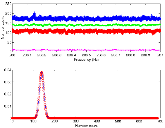
Figure 3: Top: maximum, mean, minimum and standard deviation of the number count of all the Hough maps in the frequency band 206-207 Hz. The data corresponds to L1 for the entire S2 run using 687 SFTs with a time baseline of 30 minutes. Bottom: the solid line corresponds to the L1 number-count distribution obtained in that band, and in red circles the theoretical expected binomial distribution for 687 SFTs and a peak selection probability of $20\%$.

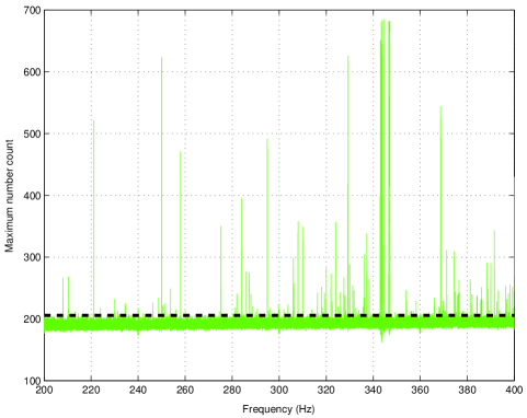
Figure 4: Graph of the L1 maximum number count per frequency analyzed, maximized over all spin-down values and sky locations. The dash-dotted line is the corresponding threshold $n_{\textrm{\mbox{\tiny{th}}}}$ for a false alarm $\alpha$ of $10^{-10}$.

As an illustrative example, some results of the Hough search in a 1 Hz frequency band are shown in figure 3. The first panel of this figure shows, for every frequency bin, the maximum, minimum, mean and standard deviation of the number counts for all sky-locations and all spindown values. As expected, the mean is approximately $Nq=0.2\times 687\approx 137$. Similarly, as expected, the standard deviation is $\sqrt{q(1-q)N}\approx 10$. The second panel of figure 3 shows the distribution of number counts in this band and compares it with the expected binomial distribution in the absence of any signal. We find excellent agreement with the expected binomial distribution, and this is true in all frequency bands which are relatively free of spectral disturbances.

Figure 4 shows the largest number count obtained for every frequency bin (i.e. the maximum number count over all sky-locations and spindown values for a given frequency value). As this figure shows, several environmental and instrumental noise sources are present. The sources of these disturbances are mostly understood. They consist of broad $60$Hz power lines, multiples of $16$Hz due to the data acquisition system, and the violin modes of the mirror suspensions in a neighborhood of $345$Hz. The 60Hz lines are rather broad, with a width of about $\pm 0.5$Hz, while the 16Hz data acquisition lines are confined to a single frequency bin. In addition to the above disturbances, we also observe a large number of multiples of $0.25$Hz. While these lines are known to be instrumental, their exact physical origin is yet to be determined.

6 Pipeline validation with hardware signal injections

Two artificial pulsar signals were injected for a duration of 12 hours at the end of the S2 run into all three LIGO interferometers. These injections were designed to give an end-to-end validation of the search pipeline starting from as far up the observing chain as possible.

The two artificial signals were injected at frequencies of 1279.123 Hz (P1) and 1288.901 Hz (P2) with spindown rates of zero and $-10^{-8}$ Hz s^-1 respectively, and amplitudes $h_{0}$ of $2\times 10^{-21}$. The signals were modulated and Doppler shifted to simulate sources at fixed positions on the sky with $\psi=0$, $\cos\iota=0$ and $\phi=0$. P1 was injected at a right acsension of 5.147 rad and a declination of 0.3767 rad, while P2 had a right ascension of 2.3457 rad and a declination of 1.2346 rad.

The resolution in the space of sky positions and frequencies are the same as in section 4, but the spin-down resolution depends on the total observation time, and this now turns out to be $-2.28624\times 10^{-8}$ Hz s^-1 for L1, $-1.77024\times 10^{-8}$ Hz s^-1 for H1, and $-1.93533\times 10^{-8}$ Hz s^-1 for H2. As before, for each intrinsic frequency we analyze 10 different spin-down values. The portion of the sky analyzed has a width of $0.5$ radians $\times$ $0.5$ radians centered around the location of the injected signals.

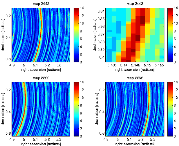
Figure 5: Hough maps for the hardware injected signal P1 in L1. Map 2442 (top-left) corresponds to 1279.123333 Hz, and contains the template which is closest to the signal. The top-right panel is a zoom of this map, showing the signal more clearly. Maps 2222 and 2662 (bottom-left and bottom-right) have a larger mismatch in frequency; they correspond to 1279.112222 Hz and 1279.134444 Hz respectively. The signal is detected in these maps also, but with a mismatched sky-location. P1 was injected at a right acsension and declination of 5.147 rad 0.3767 rad respectively. This sky-location corresponds roughly to the center of the skypatches shown in these figures.

Figure 5 shows some results for pulsar P1 using L1 data. There were 14 SFTs available in the duration when the pulsar was injected. The top left and top right panels of figure 5 shows Hough maps corresponding to the frequency and spin-down values nearest to the injected signal. Although the presence of the signal is clearly visible, 12 hours of observation time is not enough to identify the location of the source in the sky. In particular, while the signal is identified with a high number count in these hough maps, one can still identify the signal in Hough maps corresponding to different frequencies and spindowns with high number-counts, but with a mismatch in the sky location. This is shown in the bottom left and bottom right panels of 5. Similar results were found for pulsar P2 and the other detectors, thus providing an important validation of this search pipeline.

7 Conclusions

In this paper, we have described the idea of the Hough search and the search pipeline used to analyze data from the second science run of the LIGO interferometers. We have shown some outputs of the Hough search pipeline in the frequency range $200$-$400$Hz, over the whole sky, and the first spindown parameter. We have also validated the search pipeline by showing that the search can detect hardware injected pulsar signals. Work is in progress to compute astrophysical upper limits using the search pipeline presented in this paper.

The eventual role of the Hough transform is in a hierarchical scheme [9, 10]. The Hough transform could be used as a computationally inexpensive and robust method for quickly scanning large parameter space volumes and producing significant candidates for a follow-up search using a more sensitive method.

8 Acknowledgments

The authors gratefully acknowledge the support of the United States National Science Foundation for the construction and operation of the LIGO Laboratory and the Particle Physics and Astronomy Research Council of the United Kingdom, the Max-Planck-Society and the State of Niedersachsen/Germany for support of the construction and operation of the GEO600 detector. The authors also gratefully acknowledge the support of the research by these agencies and by the Australian Research Council, the Natural Sciences and Engineering Research Council of Canada, the Council of Scientific and Industrial Research of India, the Department of Science and Technology of India, the Spanish Ministerio de Educación y Ciencia, the John Simon Guggenheim Foundation, the David and Lucile Packard Foundation, the Research Corporation, and the Alfred P. Sloan Foundation.

Bibliography

Bibliography

- [1] Abbott B et al(The LIGO Scientific Collaboration) 2004 Phys. Rev. D 69 082004
- [2] —–2005 Phys. Rev. Lett. 94 181103
- [3] Astone P et al2002 Phys. Rev. D 65 042003
- [4] Krishnan B et al2004 Phys.Rev. D 70 082001
- [5] Jaranowski P, Królak A, and Schutz B F 1998 Phys. Rev. D 58 063001
- [6] Hough P V C 1959 In International Conference on High Energy Accelerators and Instrumentation CERN
- [7] —–1962 U.S. Patent 3,069,654
- [8] Illingworth J and Kittler J 1988 Computer Vision, Graphics, and Image Processing 44 87-116
- [9] Brady P R and Creighton T 2000 Phys. Rev. D 61 082001
- [10] Cutler C, Gholami I, and Krishnan B, gr-qc/0505082
- [11] Abbott B et al2004 Nucl. Instrum. Meth. A 517 154-179
- [12] Mohanty S D 2002 Class. Quantum Grav. 19 1513