Intrinsic definitions of “relative velocity” in general relativity

Abstract

Given two observers, we define the “relative velocity” of one observer with respect to the other in four different ways. All four definitions are given intrinsically, i.e. independently of any coordinate system. Two of them are given in the framework of spacelike simultaneity and, analogously, the other two are given in the framework of observed (lightlike) simultaneity. Properties and physical interpretations are discussed. Finally, we study relations between them in special relativity, and we give some examples in Schwarzschild and Robertson-Walker spacetimes.

1 Introduction

The need for a strict definition of “radial velocity” was treated at the General Assembly of the International Astronomical Union (IAU), held in 2000 (see [1], [2]), due to the ambiguity of the classic concepts in general relativity. As result, they obtained three different concepts of radial velocity: kinematic (which corresponds most closely to the line-of-sight component of space velocity), astrometric (which can be derived from astrometric observations) and spectroscopic (also called barycentric, which can be derived from spectroscopic measurements). The kinematic and astrometric radial velocities were defined using a particular reference system, called Barycentric Celestial Reference System (BCRS). The BCRS is suitable for accurate modelling of motions and events within the solar system, but it has not into account the effects produced by gravitational fields outside the solar system, since it describes an asymptotically flat metric at large distances from the Sun. Moreover, from a more theoretical point of view, these concepts can not be defined in an arbitrary spacetime since they are not intrinsic, i.e. they only have sense in the framework of the BCRS. So, in this work we are going to define them intrinsically. In fact, we obtain in a natural way four intrinsic definitions of relative velocity (and consequently, radial velocity) of one observer $\beta^{\prime}$ with respect to another observer $\beta$, following the original ideas of the IAU.

This paper has two big parts:

• The first one is formed by Sections 3 and 4, where all the concepts are defined, trying to make the paper as self-contained as possible. In Section 3, we define the kinematic and Fermi relative velocities in the framework of spacelike simultaneity (also called Fermi simultaneity), obtaining some general properties and interpretations. The kinematic relative velocity generalizes the usual concept of relative velocity when the two observers $\beta$, $\beta^{\prime}$ are at the same event. On the other hand, the Fermi relative velocity does not generalize this concept, but it is physically interpreted as the variation of the relative position of $\beta^{\prime}$ with respect to $\beta$ along the world line of $\beta$. Analogously, in Section 4, we define and study the spectroscopic and astrometric relative velocities in the framework of observed (lightlike) simultaneity.

• In the second one (Sections 5 and 6) we give some relations between these concepts in special and general relativity. In Section 5 we find general expressions, in special relativity, for the relation between kinematic and Fermi relative velocities, and between spectroscopic and astrometric relative velocities. Finally, in Section 6 we show some fundamental examples in Schwarzschild and Robertson-Walker spacetimes.

2 Preliminaries

We work in a 4-dimensional lorentzian spacetime manifold $\left(\mathcal{M},g\right)$, with $c=1$ and $\nabla$ the Levi-Civita connection, using the Landau-Lifshitz Spacelike Convention (LLSC). We suppose that $\mathcal{M}$ is a convex normal neighborhood [3]. Thus, given two events $p$ and $q$ in $\mathcal{M}$, there exists a unique geodesic joining $p$ and $q$ and there are not caustics. The parallel transport from $p$ to $q$ along this geodesic will be denoted by $\tau_{pq}$. If $\beta:I\rightarrow\mathcal{M}$ is a curve with $I\subset\mathbb{R}$ a real interval, we will identify $\beta$ with the image $\beta I$ (that is a subset in $\mathcal{M}$), in order to simplify the notation. If $u$ is a vector, then $u^{\bot}$ denotes the orthogonal space of $u$. The projection of a vector $v$ onto $u^{\bot}$ is the projection parallel to $u$. Moreover, if $x$ is a spacelike vector, then $\|x\|$ denotes the modulus of $x$. Given a pair of vectors $u,v$, we use $g\left(u,v\right)$ instead of $u^{\alpha}v_{\alpha}$. If $X$ is a vector field (typically, vector fields will be denoted by uppercase letters), $X_{p}$ denotes the unique vector of $X$ in $T_{p}\mathcal{M}$.

In general, we will say that a timelike world line $\beta$ is an observer (or a test particle). Nevertheless, we will say that a future-pointing timelike unit vector $u$ in $T_{p}\mathcal{M}$ is an observer at $p$, identifying it with its 4-velocity.

The relative velocity of an observer (or a test particle) with respect to another observer is completely well defined only when these observers are at the same event: given two observers $u$ and $u^{\prime}$ at the same event $p$, there exists a unique vector $v\in u^{\bot}$ and a unique positive real number $\gamma$ such that

$$u^{\prime}=\gamma\left(u+v\right).$$ (1)

As consequences, we have $0\leq\|v\|<1$ and $\gamma:=-g\left(u^{\prime},u\right)=\frac{1}{\sqrt{1-\|v\|^{2}}}$. We will say that $v$ is the relative velocity of $u^{\prime}$ observed by $u$, and $\gamma$ is the gamma factor corresponding to the velocity $\|v\|$. From (1), we have

$$v=\frac{1}{-g\left(u^{\prime},u\right)}u^{\prime}-u.$$ (2)

We will extend this definition of relative velocity in two different ways (kinematic and spectroscopic) for observers at different events. Moreover, we will define another two concepts of relative velocity (Fermi and astrometric) that do not extend (2) in general, but they have clear physical sense as the variation of the relative position.

A light ray is given by a lightlike geodesic $\lambda$ and a future-pointing lightlike vector field $F$ defined in $\lambda$, tangent to $\lambda$ and parallelly transported along $\lambda$ (i.e. $\nabla_{F}F=0$), called frequency (or wave) vector field of $\lambda$. Given $p\in\lambda$ and $u$ an observer at $p$, there exists a unique vector $w\in u^{\bot}$ and a unique positive real number $\nu$ such that

$$F_{p}=\nu\left(u+w\right).$$ (3)

As consequences, we have $\|w\|=1$ and $\nu=-g\left(F_{p},u\right)$. We will say that $w$ is the relative velocity of $\lambda$  observed by $u$, and $\nu$ is the frequency of $\lambda$ observed by $u$. In other words, $\nu$ is the modulus of the projection of $F_{p}$ onto $u^{\perp}$. A light ray from $q$ to $p$ is a light ray $\lambda$ such that $q$, $p\in\lambda$ and $\exp_{q}^{-1}p$ is future-pointing.

3 Relative velocity in the framework of spacelike simultaneity

The spacelike simultaneity was introduced by E. Fermi (see [4]), and it was used to define the Fermi coordinates. So, some concepts given in this section are very related to the work of Fermi, as the Fermi surfaces, the Fermi derivative or the Fermi distance. The original Fermi paper and most of the modern discussions of this notion (see [5], [6]) use a coordinate language (Fermi coordinates). On the other hand, in the present work we use a coordinate-free notation that allows us to get a better understanding of the basic concepts of the Fermi work, studying them from an intrinsic point of view and, in the next section, extending them to the framework of lightlike simultaneity.

Let $u$ be an observer at $p\in\mathcal{M}$ and $\Phi:\mathcal{M}\rightarrow\mathbb{R}$ defined by $\Phi\left(q\right):=g\left(\exp_{p}^{-1}q,u\right)$. Then, it is a submersion and the set $L_{p,u}:=\Phi^{-1}\left(0\right)$ is a regular 3-dimensional submanifold, called Landau submanifold of $\left(p,u\right)$ (see [7], [8]), also known as Fermi surface. In other words, $L_{p,u}=\exp_{p}u^{\bot}$. An event $q$ is in $L_{p,u}$ if and only if $q$ is simultaneous with $p$ in the local inertial proper system of $u$.

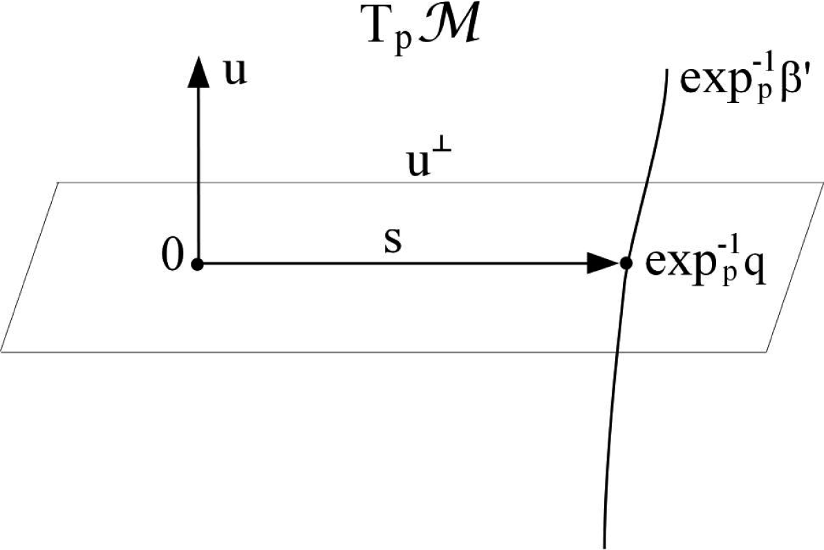
Figure 1: Scheme in $T_{p}\mathcal{M}$ of the relative position $s$ of $q$ with respect to $u$.

Definition 3.1

Given $u$ an observer at $p$, and a simultaneous event $q\in L_{p,u}$, the relative position of $q$ with respect to $u$ is $s:=\exp_{p}^{-1}q$ (see Fig. 1).

We can generalize this definition for two observers $\beta$ and $\beta^{\prime}$.

Definition 3.2

Let $\beta$, $\beta^{\prime}$ be two observers and let $U$ be the 4-velocity of $\beta$. The relative position of $\beta^{\prime}$ with respect to $\beta$ is the vector field $S$ defined on $\beta$ such that $S_{p}$ is the relative position of $q$ with respect to $U_{p}$, where $p\in\beta$ and $q$ is the unique event of $\beta^{\prime}\cap L_{p,U_{p}}$.

3.1 Kinematic relative velocity

We are going to introduce the concept of “kinematic relative velocity” of one observer $u^{\prime}$ with respect to another observer $u$ generalizing the concept of relative velocity given by (2), when the two observers are at different events.

Definition 3.3

Let $u$, $u^{\prime}$ be two observers at $p$, $q$ respectively such that $q\in L_{p,u}$. The kinematic relative velocity of $u^{\prime}$ with respect to $u$ is the unique vector $v_{\mathrm{kin}}\in u^{\bot}$ such that $\tau_{qp}u^{\prime}=\gamma\left(u+v_{\mathrm{kin}}\right)$, where $\gamma$ is the gamma factor corresponding to the velocity $\|v_{\mathrm{kin}}\|$ (see Fig. 2). So, it is given by

$$v_{\mathrm{kin}}:=\frac{1}{-g\left(\tau_{qp}u^{\prime},u\right)}\tau_{qp}u^{\prime}-u.$$ (4)

Let $s$ be the relative position of $q$ with respect to $p$, the kinematic radial velocity of $u^{\prime}$ with respect to $u$ is the component of $v_{\mathrm{kin}}$ parallel to $s$, i.e. $v_{\mathrm{kin}}^{\mathrm{rad}}:=g\left(v_{\mathrm{kin}},\frac{s}{\left\|s\right\|}\right)\frac{s}{\left\|s\right\|}$. If $s=0$ (i.e. $p=q$) then $v_{\mathrm{kin}}^{\mathrm{rad}}:=v_{\mathrm{kin}}$. On the other hand, the kinematic tangential velocity of $u^{\prime}$ with respect to $u$ is the component of $v_{\mathrm{kin}}$ orthogonal to $s$, i.e. $v_{\mathrm{kin}}^{\mathrm{tng}}:=v_{\mathrm{kin}}-v_{\mathrm{kin}}^{\mathrm{rad}}$.

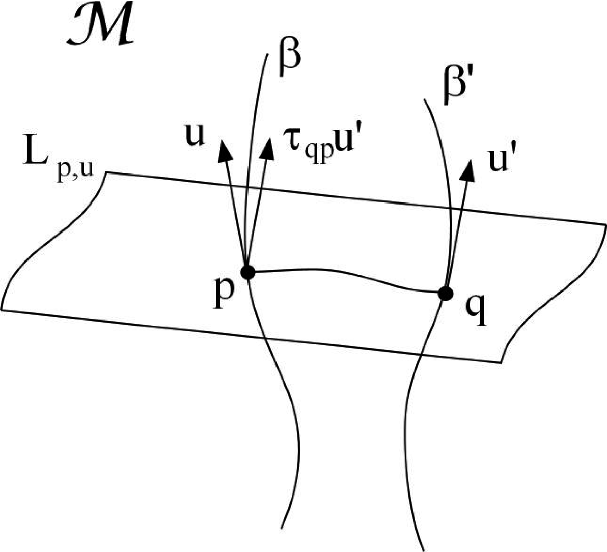
Figure 2: Scheme in $\mathcal{M}$ of the elements that involve the definition of the kinematic relative velocity of $u^{\prime}$ with respect to $u$.

So, the kinematic relative velocity of $u^{\prime}$ with respect to $u$ is the relative velocity of $\tau_{qp}u^{\prime}$ observed by $u$, in the sense of expression (2). Note that $\|v_{\mathrm{kin}}\|<1$, since the parallel transported observer $\tau_{qp}u^{\prime}$ defines an observer at $p$.

We can generalize these definitions for two observers $\beta$ and $\beta^{\prime}$.

Definition 3.4

Let $\beta$, $\beta^{\prime}$ be two observers, and let $U$, $U^{\prime}$ be the $4$-velocities of $\beta$, $\beta^{\prime}$ respectively. The kinematic relative velocity of $\beta^{\prime}$ with respect to $\beta$ is the vector field $V_{\mathrm{kin}}$ defined on $\beta$ such that $V_{\mathrm{kin}~{}p}$ is the kinematic relative velocity of $U_{q}^{\prime}$ observed by $U_{p}$ (in the sense of Definition 3.3), where $p\in\beta$ and $q$ is the unique event of $\beta^{\prime}\cap L_{p,U_{p}}$. In the same way, we define the kinematic radial velocity of $\beta^{\prime}$ with respect to $\beta$, denoted by $V_{\mathrm{kin}}^{\mathrm{rad}}$, and the kinematic tangential velocity of $\beta^{\prime}$ with respect to $\beta$, denoted by $V_{\mathrm{kin}}^{\mathrm{tng}}$.

We will say that $\beta$ is kinematically comoving with $\beta^{\prime}$ if $V_{\mathrm{kin}}=0$.

Let $V_{\mathrm{kin}}^{\prime}$ be the kinematic relative velocity of $\beta$ with respect to $\beta^{\prime}$. Then, $V_{\mathrm{kin}}=0$ if and only if $V_{\mathrm{kin}}^{\prime}=0$, i.e. the relation “to be kinematically comoving with” is symmetric and so, we can say that $\beta$ and $\beta^{\prime}$ are kinematically comoving (each one with respect to the other). Note that it is not transitive in general.

3.2 Fermi relative velocity

We are going to define the “Fermi relative velocity” as the variation of the relative position.

Definition 3.5

Let $\beta$, $\beta^{\prime}$ be two observers, let $U$ be the 4-velocity of $\beta$, and let $S$ be the relative position of $\beta^{\prime}$ with respect to $\beta$. The Fermi relative velocity of $\beta^{\prime}$ with respect to $\beta$ is the projection of $\nabla_{U}S$ onto $U^{\bot}$, i.e. it is the vector field

$$V_{\mathrm{Fermi}}:=\nabla_{U}S+g\left(\nabla_{U}S,U\right)U$$ (5)

defined on $\beta$. The right-hand side of (5) is known as the Fermi derivative. The Fermi radial velocity of $\beta^{\prime}$ with respect to $\beta$ is the component of $V_{\mathrm{Fermi}}$ parallel to $S$, i.e. $V_{\mathrm{Fermi}}^{\mathrm{rad}}:=g\left(V_{\mathrm{Fermi}},\frac{S}{\left\|S\right\|}\right)\frac{S}{\left\|S\right\|}$ if $S\neq 0$; if $S_{p}=0$ (i.e. $\beta$ and $\beta^{\prime}$ intersect at $p$) then $V_{\mathrm{Fermi}~{}p}^{\mathrm{rad}}:=V_{\mathrm{Fermi}~{}p}$. On the other hand, the Fermi tangential velocity of $\beta^{\prime}$ with respect to $\beta$ is the component of $V_{\mathrm{Fermi}}$ orthogonal to $S$, i.e. $V_{\mathrm{Fermi}}^{\mathrm{tng}}:=V_{\mathrm{Fermi}}-V_{\mathrm{Fermi}}^{\mathrm{rad}}$.

We will say that $\beta$ is Fermi-comoving with $\beta^{\prime}$ if $V_{\mathrm{Fermi}}=0$.

It is important to remark that the modulus of the vectors of $V_{\mathrm{Fermi}}$ is not necessarily smaller than one.

Since $g\left(V_{\mathrm{Fermi}},S\right)=g\left(\nabla_{U}S,S\right)$, if $S\neq 0$ we have

$$V_{\mathrm{Fermi}}^{\mathrm{rad}}=g\left(\nabla_{U}S,\frac{S}{\left\|S\right\|}\right)\frac{S}{\left\|S\right\|}.$$ (6)

The relation “to be Fermi-comoving with” is not symmetric in general.

An expression similar to (5) is given by the next proposition, that can be proved easily.

Proposition 3.1

Let $\beta$, $\beta^{\prime}$ be two observers, let $U$ be the 4-velocity of $\beta$, let $S$ be the relative position of $\beta^{\prime}$ with respect to $\beta$, and let $V_{\mathrm{Fermi}}$ be the Fermi relative velocity of $\beta^{\prime}$ with respect to $\beta$. Then $V_{\mathrm{Fermi}}=\nabla_{U}S-g\left(S,\nabla_{U}U\right)U$. Note that if $\beta$ is geodesic, then $\nabla_{U}U=0$, and hence $V_{\mathrm{Fermi}}=\nabla_{U}S$ .

If $S_{p}=0$, i.e. $\beta$ and $\beta^{\prime}$ intersect at $p$, then $V_{\mathrm{Fermi}~{}p}=\left(\nabla_{U}S\right)_{p}$. So, it does not coincide in general with the concept of relative velocity given in expression (2).

We are going to introduce a concept of distance from the concept of relative position given in Definition 3.2. This concept of distance was previously introduced by Fermi.

Definition 3.6

Let $u$ be an observer at an event $p$. Given $q$, $q^{\prime}\in L_{p,u}$, and $s$, $s^{\prime}$ the relative positions of $q$, $q^{\prime}$ with respect to $u$ respectively, the Fermi distance from $q$ to $q^{\prime}$ with respect to $u$ is the modulus of $s-s^{\prime}$, i.e. $d_{u}^{\mathrm{Fermi}}\left(q,q^{\prime}\right):=\left\|s-s^{\prime}\right\|$.

We have that $d_{u}^{\mathrm{Fermi}}$ is symmetric, positive-definite and satisfies the triangular inequality. So, it has all the properties that must verify a topological distance defined on $L_{p,u}$. As a particular case, if $q^{\prime}=p$ we have

$$d_{u}^{\mathrm{Fermi}}\left(q,p\right)=\left\|s\right\|=\left(g\left(\exp_{p}^{-1}q,\exp_{p}^{-1}q\right)\right)^{1/2}.$$ (7)

The next proposition shows that the concept of Fermi distance is the arclength parameter of a spacelike geodesic, and it can be proved taking into account the properties of the exponential map (see [3]).

Proposition 3.2

Let $u$ be an observer at an event $p$. Given $q\in L_{p,u}$ and $\alpha$ the unique geodesic from $p$ to $q$, if we parameterize $\alpha$ by its arclength such that $\alpha\left(0\right)=p$, then $\alpha\left(d_{u}^{\mathrm{Fermi}}\left(q,p\right)\right)=q$.

Definition 3.7

Let $\beta$, $\beta^{\prime}$ be two observers and let $S$ be the relative position of $\beta^{\prime}$ with respect to $\beta$. The Fermi distance from $\beta^{\prime}$ to $\beta$ with respect to $\beta$ is the scalar field $\left\|S\right\|$ defined in $\beta$.

We are going to characterize the Fermi radial velocity in terms of the Fermi distance.

Proposition 3.3

Let $\beta$, $\beta^{\prime}$ be two observers, let $S$ be the relative position of $\beta^{\prime}$ with respect to $\beta$, and let $U$ be the 4-velocity of $\beta$. If $S\neq 0$, the Fermi radial velocity of $\beta^{\prime}$ with respect to $\beta$ reads $V_{\mathrm{Fermi}}^{\mathrm{rad}}=U\left(\left\|S\right\|\right)\frac{S}{\left\|S\right\|}$.

By Definition 3.7 and Proposition 3.3, the Fermi radial velocity of $\beta^{\prime}$ with respect to $\beta$ is the rate of change of the Fermi distance from $\beta^{\prime}$ to $\beta$ with respect to $\beta$. So, if we parameterize $\beta$ by its proper time $\tau$, the Fermi radial velocity of $\beta^{\prime}$ with respect to $\beta$ at $p=\beta\left(\tau_{0}\right)$ is given by $V_{\mathrm{Fermi}~{}p}^{\mathrm{rad}}=\frac{\mathrm{d}\left(\left\|S\right\|\circ\beta\right)}{\mathrm{d}\tau}\left(\tau_{0}\right)\frac{S_{p}}{\left\|S_{p}\right\|}$, where $\left\|S\right\|\circ\beta$ is the Fermi distance as a function of $\tau$.

4 Relative velocity in the framework of lightlike simultaneity

The lightlike (or observed) simultaneity is based on “what an observer is really observing” and it provides an appropriate framework to study optical phenomena and observational cosmology (see [9]).

Let $p\in\mathcal{M}$ and $\varphi:\mathcal{M}\rightarrow\mathbb{R}$ defined by $\varphi\left(q\right):=g\left(\exp_{p}^{-1}q,\exp_{p}^{-1}q\right)$. Then, it is a submersion and the set

$$E_{p}:=\varphi^{-1}\left(0\right)-\left\{p\right\}$$ (8)

is a regular 3-dimensional submanifold, called horismos submanifold of $p$ (see [8], [10]). An event $q$ is in $E_{p}$ if and only if $q\neq p$ and there exists a lightlike geodesic joining $p$ and $q$. $E_{p}$ has two connected components, $E_{p}^{-}$ and $E_{p}^{+}$ [11]; $E_{p}^{-}$ (respectively $E_{p}^{+}$) is the past-pointing (respectively future-pointing) horismos submanifold of $p$, and it is the connected component of (8) in which, for each event $q\in E_{p}^{-}$ (respectively $q\in E_{p}^{+}$), the preimage $\exp_{p}^{-1}q$ is a past-pointing (respectively future-pointing) lightlike vector. In other words, $E_{p}^{-}=\exp_{p}C_{p}^{-}$, and $E_{p}^{+}=\exp_{p}C_{p}^{+}$, where $C_{p}^{-}$ and $C_{p}^{+}$ are the past-pointing and the future-pointing light cones of $T_{p}\mathcal{M}$ respectively.

This section is analogous to Section 3, but using $E_{p}^{-}$ instead of $L_{p,u}$.

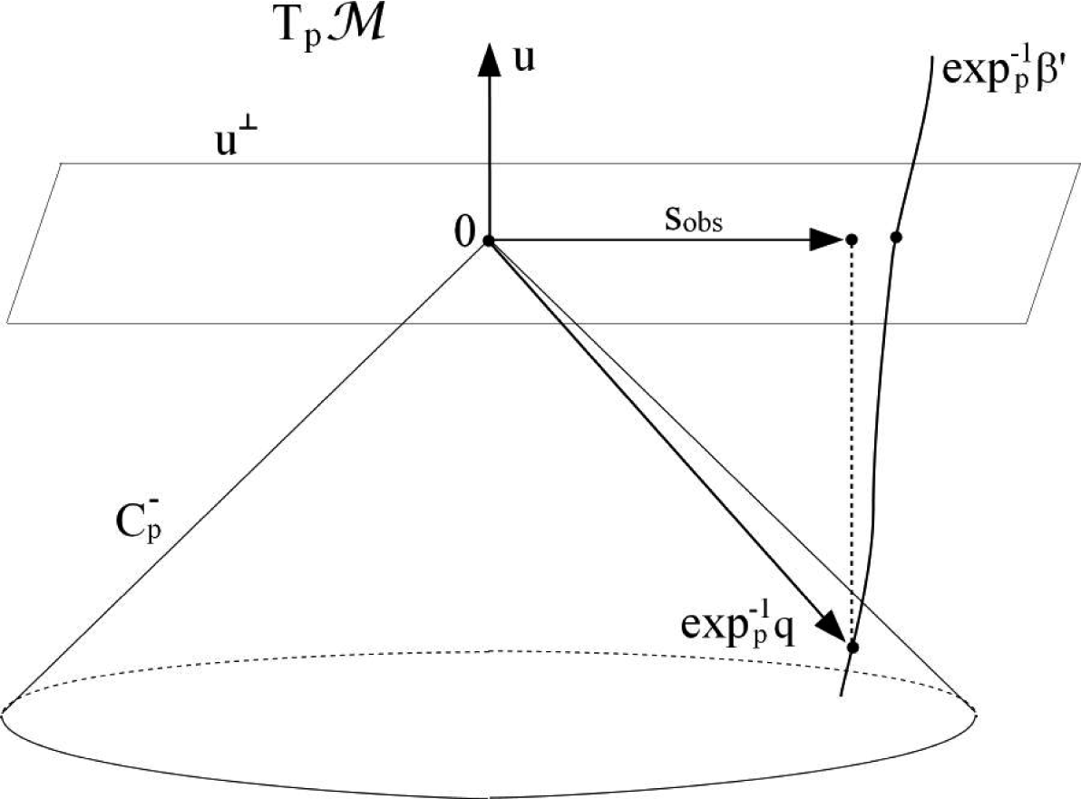
Figure 3: Scheme in $T_{p}\mathcal{M}$ of the relative position $s_{\mathrm{obs}}$ of $q$ observed by $u$.

Definition 4.1

Given $u$ an observer at $p$, and an observed event $q\in E_{p}^{-}\cup\left\{p\right\}$, the relative position of $q$ observed by $u$ (or the observed relative position of $q$ with respect to $u$) is the projection of $\exp_{p}^{-1}q$ onto $u^{\bot}$ (see Fig. 3), i.e. $s_{\mathrm{obs}}:=\exp_{p}^{-1}q+g\left(\exp_{p}^{-1}q,u\right)u$.

We can generalize this definition for two observers $\beta$ and $\beta^{\prime}$.

Definition 4.2

Let $\beta$, $\beta^{\prime}$ be two observers and let $U$ be the 4-velocity of $\beta$. The relative position of $\beta^{\prime}$ observed by $\beta$ is the vector field $S_{\mathrm{obs}}$ defined in $\beta$ such that $S_{\mathrm{obs}~{}p}$ is the relative position of $q$ observed by $U_{p}$, where $p\in\beta$ and $q$ is the unique event of $\beta^{\prime}\cap E_{p}^{-}$.

4.1 Spectroscopic relative velocity

In a previous work (see [12]), we defined a concept of relative velocity of an observer observed by another observer in the framework of lightlike simultaneity. We are going to rename this concept as “spectroscopic relative velocity”, and to review its properties in the context of this work.

Definition 4.3

Let $u$, $u^{\prime}$ be two observers at $p$, $q$ respectively such that $q\in E_{p}^{-}$ and let $\lambda$ be a light ray from $q$ to $p$. The spectroscopic relative velocity of $u^{\prime}$ observed by $u$ is the unique vector $v_{\mathrm{spec}}\in u^{\bot}$ such that $\tau_{qp}u^{\prime}=\gamma\left(u+v_{\mathrm{spec}}\right)$, where $\gamma$ is the gamma factor corresponding to the velocity $\|v_{\mathrm{spec}}\|$ (see Fig. 4). So, it is given by

$$v_{\mathrm{spec}}:=\frac{1}{-g\left(\tau_{qp}u^{\prime},u\right)}\tau_{qp}u^{\prime}-u.$$ (9)

We define the spectroscopic radial and tangential velocity of $u^{\prime}$ observed by $u$ analogously to Definition 3.3, using $s_{\mathrm{obs}}$ (see Definition 4.1) instead of $s$.

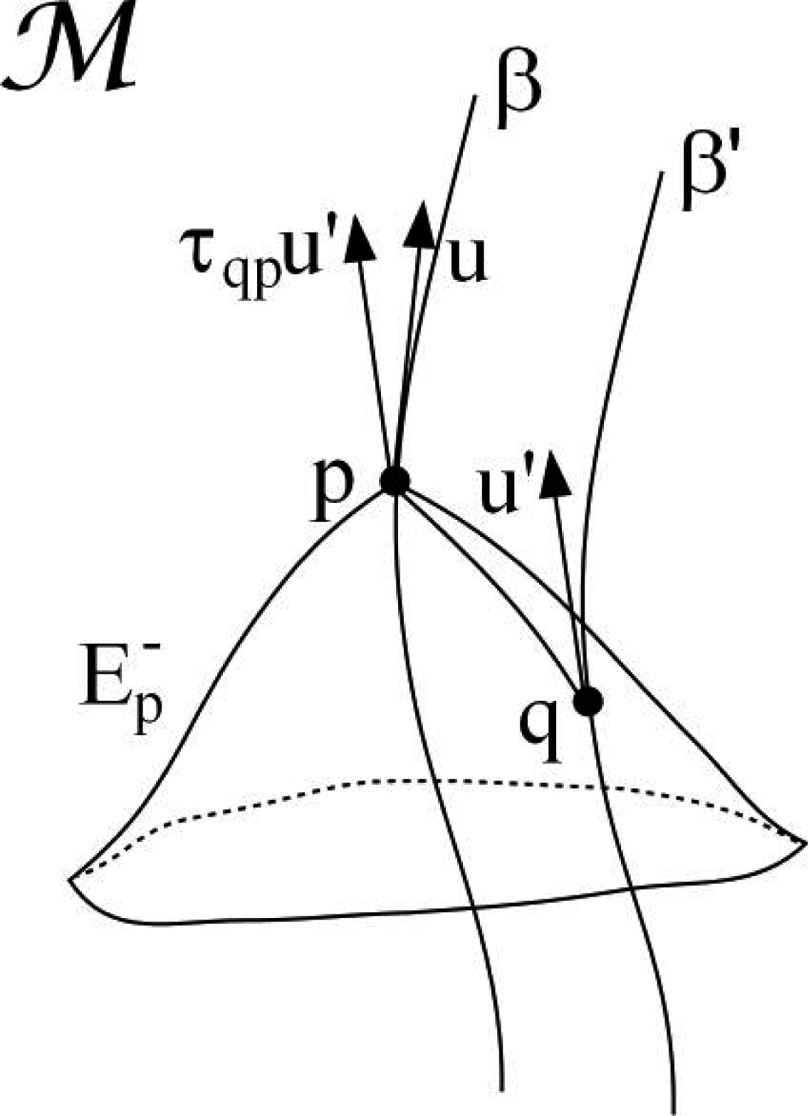
Figure 4: Scheme in $\mathcal{M}$ of the elements that involve the definition of the spectroscopic relative velocity of $u^{\prime}$ observed by $u$.

So, the spectroscopic relative velocity of $u^{\prime}$ observed by $u$ is the relative velocity of $\tau_{qp}u^{\prime}$ observed by $u$, in the sense of expression (2), and $\|v_{\mathrm{spec}}\|<1$.

Note that if $w$ is the relative velocity of $\lambda$ observed by $u$ (see (3)), then $w=-\frac{s_{\mathrm{obs}}}{\left\|s_{\mathrm{obs}}\right\|}$, and so

$$v_{\mathrm{spec}}^{\mathrm{rad}}=g\left(v_{\mathrm{spec}},w\right)w.$$ (10)

We can generalize these definitions for two observers $\beta$ and $\beta^{\prime}$.

Definition 4.4

Let $\beta$, $\beta^{\prime}$ be two observers, we define $V_{\mathrm{spec}}$ (the spectroscopic relative velocity of $\beta^{\prime}$ observed by $\beta$) and its radial and tangential components analogously to Definition 3.4, using $E_{p}^{-}$ instead of $L_{p,U_{p}}$.

We will say that $\beta$ is spectroscopically comoving with $\beta^{\prime}$ if $V_{\mathrm{spec}}=0$.

The relation “to be spectroscopically comoving with” is not symmetric in general.

The following result can be found in [12].

Proposition 4.1

Let $\lambda$ be a light ray from $q$ to $p$ and let $u$, $u^{\prime}$ be two observers at $p$, $q$ respectively. Then

$$\nu^{\prime}=\gamma\left(1-g\left(v_{\mathrm{spec}},w\right)\right)\nu,$$ (11)

where $\nu$, $\nu^{\prime}$ are the frequencies of $\lambda$ observed by $u$, $u^{\prime}$ respectively, $v_{\mathrm{spec}}$ is the spectroscopic relative velocity of $u^{\prime}$ observed by $u$, $w$ is the relative velocity of $\lambda$ observed by $u$, and $\gamma$ is the gamma factor corresponding to the velocity $\|v_{\mathrm{spec}}\|$.

Expression (11) is the general expression for Doppler effect (that includes gravitational redshift, see [12]). Therefore, if $\beta$ is spectroscopically comoving with $\beta^{\prime}$, and $\lambda$ is a light ray from $\beta^{\prime}$ to $\beta$, then, by (11), we have that $\beta$ and $\beta^{\prime}$ observe $\lambda$ with the same frequency. So, if $\beta^{\prime}$ emits $n$ light rays in a unit of its proper time, then $\beta$ observes also $n$ light rays in a unit of its proper time. Hence, $\beta$ observes that $\beta^{\prime}$ uses the “same clock” as its.

Taking into account (10), expression (11) can be written in the form

$$\nu^{\prime}=\frac{1\pm\|v_{\mathrm{spec}}^{\mathrm{rad}}\|}{\sqrt{1-\|v_{\mathrm{spec}}\|^{2}}}\nu,$$ (12)

where we choose “$+$” if $g\left(v_{\mathrm{spec}},w\right)<0$ (i.e. if $u^{\prime}$ is moving away from $u$), and we choose “$-$” if $g\left(v_{\mathrm{spec}},w\right)>0$ (i.e. if $u^{\prime}$ is getting closer to $u$).

Remark 4.1

We can not deduce $v_{\mathrm{spec}}$ from the shift, $\nu^{\prime}/\nu$, unless we make some assumptions (like considering negligible the tangential component of $v_{\mathrm{spec}}$, as we will see in Remark 4.2). For instance, if $\nu^{\prime}/\nu=1$ then $v_{\mathrm{spec}}$ is not necessarily zero. Let us study this particular case: by (11) we have

$$1=\frac{\nu^{\prime}}{\nu}=\frac{1-g\left(v_{\mathrm{spec}},w\right)}{\sqrt{1-\|v_{\mathrm{spec}}\|^{2}}}\longrightarrow g\left(v_{\mathrm{spec}},w\right)=1-\sqrt{1-\|v_{\mathrm{spec}}\|^{2}}.$$

Since $\left(1-\sqrt{1-\|v_{\mathrm{spec}}\|^{2}}\right)\geq 0$, it is necessary that $g\left(v_{\mathrm{spec}},w\right)\geq 0$, i.e. the observed object has to be getting closer to the observer. In this case, by (12) we have $\|v_{\mathrm{spec}}^{\mathrm{rad}}\|=1-\sqrt{1-\|v_{\mathrm{spec}}\|^{2}}$. So, it is possible that $\nu^{\prime}/\nu=1$ and $v_{\mathrm{spec}}\neq 0$ if the observed object is getting closer to the observer. On the other hand, if the observed object is moving away from the observer then $\nu^{\prime}/\nu=1$ if and only if $v_{\mathrm{spec}}=0$. That is, for objects moving away, the shift is always redshift; and for objects getting closer, the shift can be blueshift, 1, or redshift.

Remark 4.2

If we suppose that $v_{\mathrm{spec}}^{\mathrm{tng}}=0$, i.e. $v_{\mathrm{spec}}=v_{\mathrm{spec}}^{\mathrm{rad}}=kw$ with $k\in\left]-1,1\right[$, then we can deduce $v_{\mathrm{spec}}$ from the shift $\nu^{\prime}/\nu$:

$$\frac{\nu^{\prime}}{\nu}=\frac{1-g\left(v_{\mathrm{spec}},w\right)}{\sqrt{1-\|v_{\mathrm{spec}}\|^{2}}}=\frac{1-k}{\sqrt{1-k^{2}}}=\frac{\sqrt{1-k}}{\sqrt{1+k}}\longrightarrow k=\frac{1-\left(\frac{\nu^{\prime}}{\nu}\right)^{2}}{1+\left(\frac{\nu^{\prime}}{\nu}\right)^{2}},$$

and hence

$$v_{\mathrm{spec}}=\left(\frac{1-\left(\frac{\nu^{\prime}}{\nu}\right)^{2}}{1+\left(\frac{\nu^{\prime}}{\nu}\right)^{2}}\right)w=-\left(\frac{1-\left(\frac{\nu^{\prime}}{\nu}\right)^{2}}{1+\left(\frac{\nu^{\prime}}{\nu}\right)^{2}}\right)\frac{s_{\mathrm{obs}}}{\left\|s_{\mathrm{obs}}\right\|}.$$ (13)

4.2 Astrometric relative velocity

We are going to define the “astrometric relative velocity” as the variation of the observed relative position.

Definition 4.5

Let $\beta$, $\beta^{\prime}$ be two observers, we define $V_{\mathrm{ast}}$ (the astrometric relative velocity of $\beta^{\prime}$ observed by $\beta$) and its radial and tangential components analogously to Definition 3.5, using $S_{\mathrm{obs}}$ (see Definition 4.2) instead of $S$. So,

$$V_{\mathrm{ast}}:=\nabla_{U}S_{\mathrm{obs}}+g\left(\nabla_{U}S_{\mathrm{obs}},U\right)U,$$ (14)

where $U$ is the 4-velocity of $\beta$.

We will say that $\beta$ is astrometrically comoving with $\beta^{\prime}$ if $V_{\mathrm{ast}}=0$.

It is important to remark that the modulus of the vectors of $V_{\mathrm{ast}}$ is not necessarily smaller than one.

Analogously to (6), since $g\left(V_{\mathrm{ast}},S_{\mathrm{obs}}\right)=g\left(\nabla_{U}S_{\mathrm{obs}},S_{\mathrm{obs}}\right)$, if $S_{\mathrm{obs}}\neq 0$ we have

$$V_{\mathrm{ast}}^{\mathrm{rad}}=g\left(\nabla_{U}S_{\mathrm{obs}},\frac{S_{\mathrm{obs}}}{\left\|S_{\mathrm{obs}}\right\|}\right)\frac{S_{\mathrm{obs}}}{\left\|S_{\mathrm{obs}}\right\|}.$$ (15)

The relation “to be astrometrically comoving with” is not symmetric in general.

An expression similar to (14) is given by the next proposition, which proof is analogous to the proof of Proposition 3.1.

Proposition 4.2

Let $\beta$, $\beta^{\prime}$ be two observers, let $U$ be the 4-velocity of $\beta$, let $S_{\mathrm{obs}}$ be the relative position of $\beta^{\prime}$ observed by $\beta$, and let $V_{\mathrm{ast}}$ be the astrometric relative velocity of $\beta^{\prime}$ observed by $\beta$. Then $V_{\mathrm{ast}}=\nabla_{U}S_{\mathrm{obs}}-g\left(S_{\mathrm{obs}},\nabla_{U}U\right)U$. Note that if $\beta$ is geodesic, then $\nabla_{U}U=0$, and hence $V_{\mathrm{ast}}=\nabla_{U}S_{\mathrm{obs}}$.

If $S_{\mathrm{obs}~{}p}=0$, i.e. $\beta$ and $\beta^{\prime}$ intersect at $p$, then $V_{\mathrm{ast}~{}p}=\left(\nabla_{U}S_{\mathrm{obs}}\right)_{p}$. So, it does not coincide in general with the concept of relative velocity given in (2).

We are going to introduce another concept of distance from the concept of observed relative position given in Definition 4.1. This distance was previously introduced in [13] and studied in [12], and it plays a basic role for the construction of optical coordinates whose relevance for cosmology was stressed in many articles by G. Ellis and his school (see [9]).

Definition 4.6

Let $u$ be an observer at an event $p$. Given $q$, $q^{\prime}\in E_{p}^{-}\cup\left\{p\right\}$, and $s_{\mathrm{obs}}$, $s_{\mathrm{obs}}^{\prime}$ the relative positions of $q$, $q^{\prime}$ observed by $u$ respectively, the affine distance from $q$ to $q^{\prime}$ observed by $u$ is the modulus of $s_{\mathrm{obs}}-s_{\mathrm{obs}}^{\prime}$, i.e. $d_{u}^{\mathrm{aff}}\left(q,q^{\prime}\right):=\left\|s_{\mathrm{obs}}-s_{\mathrm{obs}}^{\prime}\right\|$.

We have that $d_{u}^{\mathrm{aff}}$ is symmetric, positive-definite and satisfies the triangular inequality. So, it has all the properties that must verify a topological distance defined on $E_{p}^{-}\cup\left\{p\right\}$. As a particular case, if $q^{\prime}=p$ we have

$$d_{u}^{\mathrm{aff}}\left(q,p\right)=\left\|s_{\mathrm{obs}}\right\|=g\left(\exp_{p}^{-1}q,u\right).$$ (16)

The next proposition shows that the concept of affine distance is according to the concept of “length” (or “time”) parameter of a lightlike geodesic for an observer, and it is proved in [12].

Proposition 4.3

Let $\lambda$ be a light ray from $q$ to $p$, let $u$ be an observer at $p$, and let $w$ be the relative velocity of $\lambda$ observed by $u$. If we parameterize $\lambda$ affinely (i.e. the vector field tangent to $\lambda$ is parallelly transported along $\lambda$) such that $\lambda\left(0\right)=p$ and $\overset{.}{\lambda}\left(0\right)=-\left(u+w\right)$, then $\lambda\left(d_{u}^{\mathrm{aff}}\left(q,p\right)\right)=q$.

Definition 4.7

Let $\beta$, $\beta^{\prime}$ be two observers and let $S_{\mathrm{obs}}$ be the relative position of $\beta^{\prime}$ observed by $\beta$. The affine distance from $\beta^{\prime}$ to $\beta$ observed by $\beta$ is the scalar field $\left\|S_{\mathrm{obs}}\right\|$ defined in $\beta$.

We are going to characterize the astrometric radial velocity in terms of the affine distance. The proof of the next proposition is analogous to the proof of Proposition 3.3, taking into account expression (15).

Proposition 4.4

Let $\beta$, $\beta^{\prime}$ be two observers, let $S_{\mathrm{obs}}$ be the relative position of $\beta^{\prime}$ observed by $\beta$, and let $U$ be the 4-velocity of $\beta$. If $S_{\mathrm{obs}}\neq 0$, the astrometric radial velocity of $\beta^{\prime}$ observed by $\beta$ reads $V_{\mathrm{ast}}^{\mathrm{rad}}=U\left(\left\|S_{\mathrm{obs}}\right\|\right)\frac{S_{\mathrm{obs}}}{\left\|S_{\mathrm{obs}}\right\|}$.

By Definition 4.7 and Proposition 4.4, the astrometric radial velocity of $\beta^{\prime}$ observed by $\beta$ is the rate of change of the affine distance from $\beta^{\prime}$ to $\beta$ observed by $\beta$. So, if we parameterize $\beta$ by its proper time $\tau$, the astrometric radial velocity of $\beta^{\prime}$ observed by $\beta$ at $p=\beta\left(\tau_{0}\right)$ is given by $V_{\mathrm{ast}~{}p}^{\mathrm{rad}}=\frac{\mathrm{d}\left(\left\|S_{\mathrm{obs}}\right\|\circ\beta\right)}{\mathrm{d}\tau}\left(\tau_{0}\right)\frac{S_{\mathrm{obs}~{}p}}{\left\|S_{\mathrm{obs}~{}p}\right\|}$, where $\left\|S_{\mathrm{obs}}\right\|\circ\beta$ is the affine distance as a function of $\tau$.

5 Special Relativity

In this section, we are going to work in the Minkowski spacetime, considering $\beta$, $\beta^{\prime}$ two observers with 4-velocities $U$, $U^{\prime}$ respectively. The goal is to find expressions for $V_{\mathrm{Fermi}}$ and $V_{\mathrm{ast}}$ in terms of $U$, $\nabla_{U}U$, $U^{\prime}$, $S$ and $S_{\mathrm{obs}}$, i.e. without $\nabla_{U}S$, $\nabla_{U}S_{\mathrm{obs}}$, or any term involving the evolution of $S$, $S_{\mathrm{obs}}$.

Proposition 5.1

Let $S$ be the relative position of $\beta^{\prime}$ with respect to $\beta$, and let $V_{\mathrm{Fermi}}$ be the Fermi relative velocity of $\beta^{\prime}$ with respect to $\beta$. Then

$$V_{\mathrm{Fermi}}=\left(1+g\left(S,\nabla_{U}U\right)\right)\left(\frac{1}{-g\left(U^{\prime},U\right)}U^{\prime}-U\right),$$ (17)

where $V_{\mathrm{Fermi}}$, $U$, $S$, $\nabla_{U}U$ are evaluated at an event $p$ of $\beta$, and $U^{\prime}$ is evaluated at the event $q=\beta^{\prime}\cap L_{p,U_{p}}$.

Proof.

We are going to consider the observers parameterized by their proper times. Let $p=\beta\left(\tau\right)$ be an event of $\beta$, let $u\left(\tau\right)$ be the 4-velocity of $\beta$ at $p$, and let $q=\beta^{\prime}\left(\tau^{\prime}\left(\tau\right)\right)$ be the event of $\beta^{\prime}$ such that $g\left(u\left(\tau\right),q-p\right)=0$ (note that the Minkowski spacetime has an affine structure, and $q-p$ denotes the vector which joins $p$ and $q$). So, $\tau^{\prime}\left(\tau\right)$ is the proper time of $q=\beta^{\prime}\cap L_{p,u}$, and the relative position of $q$ with respect to $u$, denoted by $s$, is $q-p$. If $u^{\prime}\left(\tau^{\prime}\right)$ is the 4-velocity of $\beta^{\prime}$ at $q$, then

$$s\left(\tau\right)=\beta^{\prime}\left(\tau^{\prime}\left(\tau\right)\right)-\beta\left(\tau\right)\,\Longrightarrow\,\dot{s}=u^{\prime}\left(\tau^{\prime}\right)\dot{\tau}^{\prime}-u,$$ (18)

where the dot denotes $\frac{d}{d\tau}$. On the other hand

$$g\left(s,u\right)=0\,\Longrightarrow\,g\left(\dot{s},u\right)+g\left(s,\dot{u}\right)=0.$$ (19)

Applying (18) in (19) we have

$$g\left(u^{\prime}\left(\tau^{\prime}\right)\dot{\tau}^{\prime}-u,u\right)+g\left(s,\dot{u}\right)=0\,\Longrightarrow\,\dot{\tau}^{\prime}=\frac{1+g\left(s,\dot{u}\right)}{-g\left(u^{\prime}\left(\tau^{\prime}\right),u\right)}.$$ (20)

Combining (18) and (20), we obtain

$$\dot{s}=\frac{1+g\left(s,\dot{u}\right)}{-g\left(u^{\prime}\left(\tau^{\prime}\right),u\right)}u^{\prime}\left(\tau^{\prime}\right)-u.$$ (21)

Let $U$, $U^{\prime}$ be the 4-velocities of $\beta$ and $\beta^{\prime}$ respectively, and let $S$ be the relative position of $\beta^{\prime}$ with respect to $\beta$. Then, from (21) we have

$$\nabla_{U}S=\frac{1+g\left(S,\nabla_{U}U\right)}{-g\left(U^{\prime},U\right)}U^{\prime}-U,$$ (22)

where $U$, $S$, $\nabla_{U}U$, $\nabla_{U}S$ are evaluated at $p$, and $U^{\prime}$ is evaluated at $q$. So, by Proposition 3.1 and expression (22), the Fermi relative velocity $V_{\mathrm{Fermi}}$ of $\beta^{\prime}$ with respect to $\beta$ is given by

$$V_{\mathrm{Fermi}} = \nabla_{U}S-g\left(S,\nabla_{U}U\right)U$$

$$= \left(1+g\left(S,\nabla_{U}U\right)\right)\left(\frac{1}{-g\left(U^{\prime},U\right)}U^{\prime}-U\right),$$

where $V_{\mathrm{Fermi}}$, $U$, $S$, $\nabla_{U}U$ are evaluated at $p$, and $U^{\prime}$ is evaluated at $q$. ∎

Taking into account the expression of the kinematic relative velocity given in (4), we obtain the next corollary:

Corollary 5.1

The Fermi relative velocity of $\beta^{\prime}$ with respect to $\beta$ reads

$$V_{\mathrm{Fermi}}=\left(1+g\left(S,\nabla_{U}U\right)\right)V_{\mathrm{kin}}.$$ (23)

So, $V_{\mathrm{Fermi}}$ and $V_{\mathrm{kin}}$ are proportional. Moreover, if $\beta$ is geodesic, then $V_{\mathrm{Fermi}}=V_{\mathrm{kin}}$.

Proposition 5.2

Let $S_{\mathrm{obs}}$ be the relative position of $\beta^{\prime}$ observed by $\beta$, and let $V_{\mathrm{ast}}$ be the astrometric relative velocity of $\beta^{\prime}$ with respect to $\beta$. Then

$$V_{\mathrm{ast}}=\frac{1}{g\left(U^{\prime},\frac{S_{\mathrm{obs}}}{\|S_{\mathrm{obs}}\|}-U\right)}\left(U^{\prime}+g\left(U^{\prime},U\right)U\right)+\|S_{\mathrm{obs}}\|\nabla_{U}U,$$ (24)

where $V_{\mathrm{ast}}$, $U$, $S_{\mathrm{obs}}$, $\nabla_{U}U$ are evaluated at an event $p$ of $\beta$, and $U^{\prime}$ is evaluated at the event $q=\beta^{\prime}\cap E^{-}_{p}$.

Proof.

We are going to consider the observers parameterized by their proper times. Let $p=\beta\left(\tau\right)$ be an event of $\beta$, let $u\left(\tau\right)$ be the 4-velocity of $\beta$ at $p$, and let $q=\beta^{\prime}\left(\tau^{\prime}\left(\tau\right)\right)$ be the event of $\beta^{\prime}$ such that $g\left(q-p,q-p\right)=0$ (note that the Minkowski spacetime has an affine structure, and $q-p$ denotes the vector which joins $p$ and $q$). So, $\tau^{\prime}\left(\tau\right)$ is the proper time of $q=\beta^{\prime}\cap E^{-}_{p}$, and the relative position of $q$ observed by $u$, denoted by $s_{\textrm{obs}}$, is the projection of $q-p$ onto $u^{\bot}$. Let us denote $s_{\mathrm{obs}}$ by $s$ for the shake of readability. Hence

$$s\left(\tau\right)=\beta^{\prime}\left(\tau^{\prime}\left(\tau\right)\right)-\beta\left(\tau\right)+\|s\left(\tau\right)\|u,$$ (25)

where $\|s\|=\sqrt{g\left(s,s\right)}$ is the affine distance from $p$ to $q$. If $u^{\prime}\left(\tau^{\prime}\right)$ is the 4-velocity of $\beta^{\prime}$ at $q$, deriving (25) with respect to $\tau$ we obtain

$$\dot{s}=u^{\prime}\left(\tau^{\prime}\right)\dot{\tau}^{\prime}-u+g\left(\dot{s},\frac{s}{\|s\|}\right)u+\|s\|\dot{u},$$ (26)

where the dot denotes $\frac{d}{d\tau}$. Taking into account that $g\left(s,u\right)=0$ and (26), we have

$$g\left(\dot{s},\frac{s}{\|s\|}\right)=g\left(u^{\prime}\left(\tau^{\prime}\right)\dot{\tau}^{\prime}+\|s\|\dot{u},\frac{s}{\|s\|}\right)=\dot{\tau}^{\prime}g\left(u^{\prime}\left(\tau^{\prime}\right),\frac{s}{\|s\|}\right)+g\left(\dot{u},s\right),$$ (27)

and hence, by (26) and (27) we obtain

$$\dot{s}=u^{\prime}\left(\tau^{\prime}\right)\dot{\tau}^{\prime}+\left(\dot{\tau}^{\prime}g\left(u^{\prime}\left(\tau^{\prime}\right),\frac{s}{\|s\|}\right)+g\left(\dot{u},s\right)-1\right)u+\|s\|\dot{u}.$$ (28)

On the other hand

$$g\left(s,u\right)=0\,\Longrightarrow\,g\left(\dot{s},u\right)+g\left(s,\dot{u}\right)=0.$$ (29)

Applying (28) in (29) and taking into account that $g\left(\dot{u},u\right)=0$, we find

$$\dot{\tau}^{\prime}=\frac{1}{g\left(u^{\prime}\left(\tau^{\prime}\right),\frac{s}{\|s\|}-u\right)}.$$ (30)

Combining (28) and (30), we obtain

$$\dot{s}=\frac{1}{g\left(u^{\prime}\left(\tau^{\prime}\right),\frac{s}{\|s\|}-u\right)}\left(u^{\prime}\left(\tau^{\prime}\right)+g\left(u^{\prime}\left(\tau^{\prime}\right),u\right)u\right)+g\left(s,\dot{u}\right)u+\|s\|\dot{u}.$$ (31)

Let $U$, $U^{\prime}$ be the 4-velocities of $\beta$ and $\beta^{\prime}$ respectively, and let $S=S_{\mathrm{obs}}$ (for the shake of readability) be the relative position of $\beta^{\prime}$ observed by $\beta$. Then, from (31) we have

$$\nabla_{U}S=\frac{1}{g\left(U^{\prime},\frac{S}{\|S\|}-U\right)}\left(U^{\prime}+g\left(U^{\prime},U\right)U\right)+g\left(S,\nabla_{U}U\right)U+\|S\|\nabla_{U}U,$$ (32)

where $U$, $S$, $\nabla_{U}U$, $\nabla_{U}S$ are evaluated at $p$, and $U^{\prime}$ is evaluated at $q$. So, by Proposition 4.2 and expression (32), the astrometric relative velocity $V_{\mathrm{ast}}$ of $\beta^{\prime}$ with respect to $\beta$ is given by

$$V_{\mathrm{ast}} = \nabla_{U}S-g\left(S,\nabla_{U}U\right)U$$

$$= \frac{1}{g\left(U^{\prime},\frac{S}{\|S\|}-U\right)}\left(U^{\prime}+g\left(U^{\prime},U\right)U\right)+\|S\|\nabla_{U}U,$$

where $V_{\mathrm{ast}}$, $U$, $S$, $\nabla_{U}U$ are evaluated at $p$, and $U^{\prime}$ is evaluated at $q$. ∎

Taking into account the expression of the spectroscopic relative velocity given in (9), we obtain the next corollary:

Corollary 5.2

The astrometric relative velocity of $\beta^{\prime}$ with respect to $\beta$ reads

$$V_{\mathrm{ast}}=\|S_{\mathrm{obs}}\|\nabla_{U}U+\frac{1}{1+g\left(V_{\mathrm{spec}},\frac{S_{\mathrm{obs}}}{\|S_{\mathrm{obs}}\|}\right)}V_{\mathrm{spec}}.$$ (33)

So, $V_{\mathrm{spec}}$ and $V_{\mathrm{ast}}$ are not proportional unless $\beta$ is geodesic.

If $\beta^{\prime}$ is geodesic then it is clear that $V_{\mathrm{spec}}=V_{\mathrm{kin}}$. Moreover, if $\beta$ is also geodesic then $V_{\mathrm{spec}}=V_{\mathrm{kin}}=V_{\mathrm{Fermi}}$.

Remark 5.1

Let us suppose that $\beta$ and $\beta^{\prime}$ intersect at $p$, let $u$, $u^{\prime}$ be the 4-velocities of $\beta$, $\beta^{\prime}$ at $p$ respectively, and let $v$ be the relative velocity of $u^{\prime}$ observed by $u$, in the sense of expression (2). Let us study the relations between $v$, $V_{\mathrm{kin}~{}p}$, $V_{\mathrm{Fermi}~{}p}$, $V_{\mathrm{spec}~{}p}$ and $V_{\mathrm{ast}~{}p}$.

It is clear that $V_{\mathrm{kin}~{}p}=V_{\mathrm{spec}~{}p}=v$, even in general relativity. Moreover, since $S_{p}=0$, by (17) we have $V_{\mathrm{Fermi}~{}p}=v$. On the other hand, since $S_{\mathrm{obs}~{}p}=0$, it is easy to prove that $V_{\mathrm{ast}~{}p}=\frac{1}{1\pm\left\|v\right\|}v$, where we choose “$+$” if we consider that $\beta^{\prime}$ is leaving from $\beta$, and we choose “$-$” if we consider that $\beta^{\prime}$ is arriving at $\beta$. Therefore, if $\beta$ and $\beta^{\prime}$ intersect at $p$, then it is not possible to write $V_{\mathrm{ast}~{}p}$ in a unique way in terms of $v$.

Example 5.1

Using rectangular coordinates $\left(t,x,y,z\right)$, let us consider the following observers: $\beta\left(\tau\right):=\left(\tau,0,0,0\right)$, and $\beta^{\prime}\left(\tau^{\prime}\right):=\left\{\begin{array}[]{l}\left(\gamma\tau^{\prime},v\gamma\tau^{\prime},0,0\right)~{}~{}{\mathrm{if}}~{}~{}\tau^{\prime}\in\left[0,\frac{1}{\gamma v}\right]\\ \\ \left(\gamma\tau^{\prime},2-v\gamma\tau^{\prime},0,0\right)~{}~{}{\mathrm{if}}~{}~{}\tau^{\prime}\in\left]\frac{1}{\gamma v},\frac{2}{\gamma v}\right]\end{array}\right.$ where $v\in\left]0,1\right[$ and $\gamma:=\frac{1}{\sqrt{1-v^{2}}}$, parameterized by their proper times. That is, $\beta$ is a stationary observer with $x=0$, $y=0$, $z=0$ and $\beta^{\prime}$ is an observer moving from $x=0$, $y=0$, $z=0$ to $x=1$, $y=0$, $z=0$ with velocity of modulus $v$ and returning (see Fig. 5). It is satisfied that

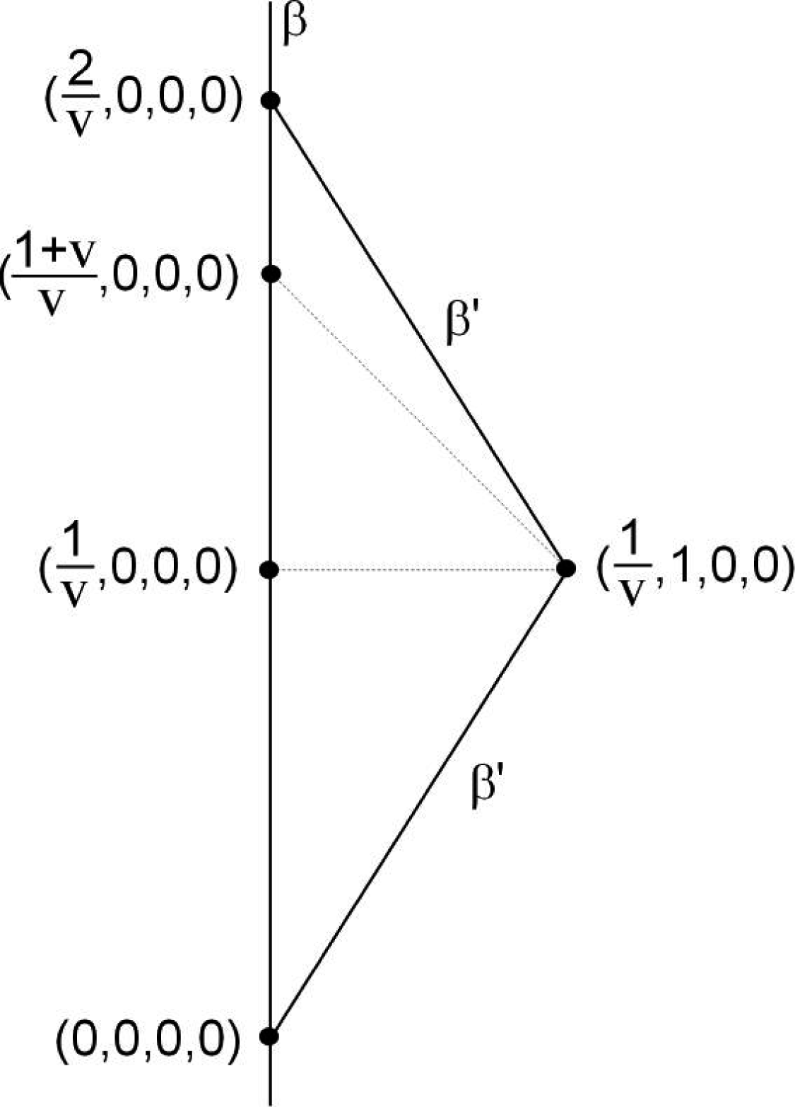
Figure 5: Scheme of the observers of Example 5.1.

$$V_{\mathrm{kin}~{}\beta\left(\tau\right)}=\left\{\begin{array}[]{l}v\left.\frac{\partial}{\partial x}\right|_{\beta\left(\tau\right)}~{}~{}\mathrm{if}~{}~{}\tau\in\left[0,\frac{1}{v}\right]\\ -v\left.\frac{\partial}{\partial x}\right|_{\beta\left(\tau\right)}~{}~{}\mathrm{if}~{}~{}\tau\in\left]\frac{1}{v},\frac{2}{v}\right]\end{array}\right.,$$

$$V_{\mathrm{spec}~{}\beta\left(\tau\right)}=\left\{\begin{array}[]{l}v\left.\frac{\partial}{\partial x}\right|_{\beta\left(\tau\right)}~{}~{}\mathrm{if}~{}~{}\tau\in\left[0,\frac{1+v}{v}\right]\\ -v\left.\frac{\partial}{\partial x}\right|_{\beta\left(\tau\right)}~{}~{}\mathrm{if}~{}~{}\tau\in\left]\frac{1+v}{v},\frac{2}{v}\right]\end{array}\right..$$

Applying (17), we obtain $V_{\mathrm{Fermi}~{}\beta\left(\tau\right)}=V_{\mathrm{kin}~{}\beta\left(\tau\right)}$. Moreover

$$S_{\mathrm{obs}~{}\beta\left(\tau\right)}=\left\{\begin{array}[]{l}\frac{v\tau}{1+v}\left.\frac{\partial}{\partial x}\right|_{\beta\left(\tau\right)}~{}~{}\mathrm{if}~{}~{}\tau\in\left[0,\frac{1+v}{v}\right]\\ \frac{2-v\tau}{1-v}\left.\frac{\partial}{\partial x}\right|_{\beta\left(\tau\right)}~{}~{}\mathrm{if}~{}~{}\tau\in\left]\frac{1+v}{v},\frac{2}{v}\right]\end{array}\right..$$

Hence, by (24) we have

$$V_{\mathrm{ast}~{}\beta\left(\tau\right)}=\left\{\begin{array}[]{l}\frac{v}{1+v}\left.\frac{\partial}{\partial x}\right|_{\beta\left(\tau\right)}~{}~{}\mathrm{if}~{}~{}\tau\in\left[0,\frac{1+v}{v}\right]\\ -\frac{v}{1-v}\left.\frac{\partial}{\partial x}\right|_{\beta\left(\tau\right)}~{}~{}\mathrm{if}~{}~{}\tau\in\left]\frac{1+v}{v},\frac{2}{v}\right]\end{array}\right..$$

Consequently, $\left\|V_{\mathrm{ast}~{}\beta\left(\tau\right)}\right\|\in\left]0,1/2\right[$ if $\tau\in\left[0,\frac{1+v}{v}\right]$, i.e. if $\beta^{\prime}$ is moving away radially. On the other hand, $\left\|V_{\mathrm{ast}~{}\beta\left(\tau\right)}\right\|\in\left]0,+\infty\right[$ if $\tau\in\left]\frac{1+v}{v},\frac{2}{v}\right]$, i.e. if $\beta^{\prime}$ is getting closer radially (see fig. 6). This corresponds to what $\beta$ observes.

Figure 6: Modulus of the relative velocities of Example 5.1 depending on the parameter $v$. The solid line represents the modulus of $V_{\mathrm{kin}}$, $V_{\mathrm{Fermi}}$ and $V_{\mathrm{spec}}$, and they are always equal to $v$. The dashed line represents the modulus of $V_{\mathrm{ast}}$ when $\beta^{\prime}$ moves away from $\beta$ (lower) and $\beta^{\prime}$ approaches $\beta$ (upper).

Example 5.2

Let us suppose that the spacetime is flat and we see an alien spaceship coming to Earth from a planet at 9 lightyears (this distance can be measured by parallax, since this method estimates the affine distance from the planet to Earth observed by someone on Earth). Let us suppose that the spaceship is coming radially, and so, we can measure the modulus of its spectroscopic relative velocity (see 4.2). Supposing that this modulus is $v=0.9$, the spaceship will take 10 years to arrive at Earth from its planet. However, since light takes 9 years to arrive at us, there is only 1 year left for the arrival of the spaceship. This result can also be obtained by using expression (24): in our case, the modulus of the astrometric relative velocity is $\frac{0.9}{1-0.9}=9$, and we will therefore observe that it takes 1 year to arrive.

Remark 5.2

There is an open problem in general relativity, that consists on finding expressions for $V_{\mathrm{Fermi}}$ and $V_{\mathrm{ast}}$ in terms of $U$, $\nabla_{U}U$, $U^{\prime}$, $S$ and $S_{\mathrm{obs}}$, analogously to Propositions 5.1 and 5.2, avoiding $\nabla_{U}S$, $\nabla_{U}S_{\mathrm{obs}}$, or any term involving the evolution of $S$, $S_{\mathrm{obs}}$. It would be very useful in the calculations of the relative velocities.

6 Examples in General Relativity

In this section, we are going to study some fundamental examples in Schwarzschild and Robertson-Walker spacetimes. See [14] for an interesting and complete study of the relative velocities of a radially receding test particle with respect to / observed by a central observer in a Schwarzschild-de Sitter spacetime.

6.1 Stationary observers in Schwarzschild spacetime

In the Schwarzschild metric with spherical coordinates

$$\mathrm{d}s^{2}=-a^{2}\left(r\right)\mathrm{d}t^{2}+\frac{1}{a^{2}\left(r\right)}\mathrm{d}r^{2}+r^{2}\left(\mathrm{d}\theta^{2}+\sin^{2}\theta\mathrm{d}\varphi^{2}\right),$$

where $a\left(r\right)=\sqrt{1-\frac{2m}{r}}$ and $r>2m$, let us consider two equatorial stationary observers, $\beta_{1}\left(\tau\right)=\left(\frac{1}{a_{1}}\tau,r_{1},\pi/2,0\right)$ and $\beta_{2}\left(\tau\right)=\left(\frac{1}{a_{2}}\tau,r_{2},\pi/2,0\right)$ with $\tau\in\mathbb{R}$, $r_{2}>r_{1}>2m$, $a_{1}:=a\left(r_{1}\right)$ and $a_{2}:=a\left(r_{2}\right)$, and let $U$ be the 4-velocity of $\beta_{2}$, i.e. $U:=\frac{1}{a_{2}}\frac{\partial}{\partial t}$. We are going to study the relative velocities of $\beta_{1}$ with respect to / observed by $\beta_{2}$.

6.1.1 Kinematic and Fermi relative velocities. Fermi distance

Let us consider the vector field $X:=a\left(r\right)\frac{\partial}{\partial r}$; it is spacelike, unit, geodesic, and orthogonal to $U$. Since $\nabla_{X}\left(\frac{1}{a\left(r\right)}\frac{\partial}{\partial t}\right)=0$, we have that the kinematic relative velocity $V_{\mathrm{kin}}$ of $\beta_{1}$ with respect to $\beta_{2}$ is given by $V_{\mathrm{kin}}=0$.

It is clear (a priori) that the relative position $S$ of $\beta_{1}$ with respect to $\beta_{2}$ is proportional to $\frac{\partial}{\partial r}$ and the proportionality factor is constant. So, it is easy to prove that $\nabla_{U}S$ is proportional to $U$ and therefore, the Fermi relative velocity $V_{\mathrm{Fermi}}$ of $\beta_{1}$ with respect to $\beta_{2}$ reads $V_{\mathrm{Fermi}}=0$.

Nevertheless, we are going to calculate the Fermi distance and $S$:

Let $\alpha\left(\sigma\right)=\left(t_{0},\alpha^{r}\left(\sigma\right),\pi/2,0\right)$ be an integral curve of $X$ such that $q:=\alpha\left(\sigma_{1}\right)\in\beta_{1}$ and $p:=\alpha\left(\sigma_{2}\right)\in\beta_{2}$, with $\sigma_{2}>\sigma_{1}$ (i.e. $\alpha\left(\sigma\right)$ is a spacelike geodesic from $q$ to $p$, parameterized by its arclength, and its tangent vector at $p$ is $X_{p}$). Then, by Proposition 3.2, the Fermi distance $d_{U_{p}}^{\mathrm{Fermi}}\left(q,p\right)$ from $q$ to $p$ with respect to $U_{p}$ is $\sigma_{2}-\sigma_{1}$. Since $\alpha$ is an integral curve of $X$, we have $\overset{.}{\alpha}^{r}\left(\sigma\right)=\sqrt{1-\frac{2m}{\alpha^{r}\left(\sigma\right)}}$. So, $\int_{r_{1}}^{r_{2}}\left(1-\frac{2m}{\alpha^{r}\left(\sigma\right)}\right)^{-1/2}\overset{.}{\alpha}^{r}\left(\sigma\right)\mathrm{d}\sigma=\sigma_{2}-\sigma_{1}$, and then

$$d_{U_{p}}^{\mathrm{Fermi}}\left(q,p\right)=2m\ln\left(\frac{\left(1-a_{1}\right)\sqrt{r_{1}}}{\left(1-a_{2}\right)\sqrt{r_{2}}}\right)+r_{2}a_{2}-r_{1}a_{1}.$$ (34)

Since (34) does not depends on $t_{0}$, the Fermi distance from $\beta_{1}$ to $\beta_{2}$ with respect to $\beta_{2}$ is also given by expression (34). Hence, by (7), the relative position $S$ of $\beta_{1}$ with respect to $\beta_{2}$ is given by

$$S=\left(2m\ln\left(\frac{\left(1-a_{2}\right)\sqrt{r_{2}}}{\left(1-a_{1}\right)\sqrt{r_{1}}}\right)+r_{1}a_{1}-r_{2}a_{2}\right)a_{2}\frac{\partial}{\partial r}.$$

6.1.2 Spectroscopic and astrometric relative velocities. Affine distance

It is easy to prove that the spectroscopic relative velocity $V_{\mathrm{spec}}$ of $\beta_{1}$ observed by $\beta_{2}$ is radial. Since the gravitational redshift is given by $\frac{a_{2}}{a_{1}}$ (see [12]), by (13) we obtain

$$V_{\mathrm{spec}}=-a_{2}\frac{a_{2}^{2}-a_{1}^{2}}{a_{2}^{2}+a_{1}^{2}}\frac{\partial}{\partial r}.$$ (35)

Expression (35) is also obtained in [12]. Since $\left\|V_{\mathrm{spec}}\right\|=\frac{a_{2}^{2}-a_{1}^{2}}{a_{2}^{2}+a_{1}^{2}}$, we have $\lim_{r_{1}\rightarrow 2m}\left\|V_{\mathrm{spec}}\right\|=1$ (see Fig. 7).

Figure 7: Modulus of $V_{\mathrm{spec}}$ of a stationary observer with $a_{1}=\sqrt{1-\frac{2m}{r_{1}}}$ observed by another stationary observer with $a_{2}=\sqrt{1-\frac{2m}{r_{2}}}=0.5$ (left) and at the exterior limit $a_{2}=1$ ($r_{2}=+\infty$) (right) in Schwarzschild spacetime. It produces the gravitational redshift.

On the other hand, it is clear (a priori) that the relative position $S_{\mathrm{obs}}$ of $\beta_{1}$ observed by $\beta_{2}$ is proportional to $\frac{\partial}{\partial r}$ and the proportionality factor is constant. So, it is easy to prove that $\nabla_{U}S_{\mathrm{obs}}$ is proportional to $U$ and therefore, the astrometric relative velocity $V_{\mathrm{ast}}$ of $\beta_{1}$ observed by $\beta_{2}$ reads $V_{\mathrm{ast}}=0$.

Nevertheless, we are going to calculate the affine distance and $S_{\mathrm{obs}}$:

In [12] it is proved (by using Proposition 4.3) that the affine distance from $\beta_{1}$ to $\beta_{2}$ observed by $\beta_{2}$ is $\frac{r_{2}-r_{1}}{a_{2}}$. Hence, by (16), the relative position $S_{\mathrm{obs}}$ of $\beta_{1}$ observed by $\beta_{2}$ is given by

$$S_{\mathrm{obs}}=\left(r_{1}-r_{2}\right)\frac{\partial}{\partial r}.$$ (36)

6.2 Free-falling observers in Schwarzschild spacetime

Let us consider a radial free-falling observer $\beta_{1}$ parameterized by the coordinate time $t$, $\beta_{1}\left(t\right)=\left(t,\beta_{1}^{r}\left(t\right),\pi/2,0\right)$. Given an event $q=\left(t_{1},r_{1},\pi/2,0\right)\in\beta_{1}$, the 4-velocity of $\beta_{1}$ at $q$ is given by

$$u_{1}=\frac{E}{a_{1}^{2}}\left.\frac{\partial}{\partial t}\right|_{q}-\sqrt{E^{2}-a_{1}^{2}}\left.\frac{\partial}{\partial r}\right|_{q},$$ (37)

where $E$ is a constant of motion given by $E:=\left(\frac{1-2m/r_{0}}{1-v_{0}^{2}}\right)^{1/2}$, $r_{0}$ is the radial coordinate at which the fall begins, $v_{0}$ is the initial velocity (see [15]), and $a_{1}:=a\left(r_{1}\right)$. Moreover, let us consider an equatorial stationary observer $\beta_{2}\left(\tau\right)=\left(\frac{1}{a_{2}}\tau,r_{2},\pi/2,0\right)$ with $\tau\in\mathbb{R}$, $r_{2}\geq r_{1}>2m$, $a_{2}:=a\left(r_{2}\right)$, and $U:=\frac{1}{a_{2}}\frac{\partial}{\partial t}$ its 4-velocity. We are going to study the relative velocities of $\beta_{1}$ with respect to / observed by $\beta_{2}$ at $p$, where $p$ will be a determined event of $\beta_{2}$.

6.2.1 Kinematic and Fermi relative velocities

Let $p=\left(t_{1},r_{2},\pi/2,0\right)$. This is the unique event of $\beta_{2}$ such that $q\in L_{p,U_{p}}$, i.e. there exists a spacelike geodesic $\alpha\left(\sigma\right)$ from $q=\alpha\left(\sigma_{1}\right)$ to $p=\alpha\left(\sigma_{2}\right)$ such that the tangent vector $\overset{.}{\alpha}\left(\sigma_{2}\right)$ is orthogonal to $U_{p}$. We can consider $\alpha\left(\sigma\right)$ parameterized by its arclength and $\sigma_{2}>\sigma_{1}$. So, $\alpha\left(\sigma\right)$ is an integral curve of the vector field $X=a\left(r\right)\frac{\partial}{\partial r}$. If we parallelly transport $u_{1}$ from $q$ to $p$ along $\alpha$ we obtain $\tau_{qp}u_{1}=\frac{E}{a_{1}a_{2}}\left.\frac{\partial}{\partial t}\right|_{p}-\frac{a_{2}}{a_{1}}\sqrt{E^{2}-a_{1}^{2}}\left.\frac{\partial}{\partial r}\right|_{p}$. By (4), the kinematic relative velocity $V_{\mathrm{kin}~{}p}$ of $\beta_{1}$ with respect to $\beta_{2}$ at $p$ reads

$$V_{\mathrm{kin}~{}p}=-a_{2}\sqrt{1-\frac{a_{1}^{2}}{E^{2}}}\left.\frac{\partial}{\partial r}\right|_{p}.$$

Since $\left\|V_{\mathrm{kin}~{}p}\right\|=\sqrt{1-\frac{a_{1}^{2}}{E^{2}}}$, it is satisfied that $\lim_{r_{1}\rightarrow 2m}\left\|V_{\mathrm{kin}~{}p}\right\|=1$. See Appendix for a deeper analysis of this function.

On the other hand, by (34), the relative position $S$ of $\beta_{1}$ with respect to $\beta_{2}$ is given by

$$S=\left(2m\ln\left(\frac{\left(1-a_{2}\right)\sqrt{r_{2}}}{\left(1-a\left(\beta_{1}^{r}\left(t\right)\right)\right)\sqrt{\beta_{1}^{r}\left(t\right)}}\right)+\beta_{1}^{r}\left(t\right)a\left(\beta_{1}^{r}\left(t\right)\right)-r_{2}a_{2}\right)a_{2}\frac{\partial}{\partial r}.$$

By (5), the Fermi relative velocity $V_{\mathrm{Fermi}}$ of $\beta_{1}$ with respect to $\beta_{2}$ reads

$$V_{\mathrm{Fermi}}=\left(\nabla_{U}S\right)^{r}\frac{\partial}{\partial r}=\frac{1}{a_{2}}\frac{\partial S^{r}}{\partial t}\frac{\partial}{\partial r}=\frac{1}{a_{2}}\frac{\overset{.}{\beta}_{1}^{r}\left(t\right)}{a\left(\beta_{1}^{r}\left(t\right)\right)}\frac{\partial}{\partial r}$$

Taking into account (37), we have $\overset{.}{\beta}_{1}^{r}\left(t_{1}\right)=-a_{1}^{2}\sqrt{1-\frac{a_{1}^{2}}{E^{2}}}$. Hence

$$V_{\mathrm{Fermi}~{}p}=-\frac{a_{1}}{a_{2}}\sqrt{1-\frac{a_{1}^{2}}{E^{2}}}\left.\frac{\partial}{\partial r}\right|_{p}.$$

Since $\left\|V_{\mathrm{Fermi}~{}p}\right\|=\frac{a_{1}}{a^{2}_{2}}\sqrt{1-\frac{a_{1}^{2}}{E^{2}}}$, it is satisfied that $\lim_{r_{1}\rightarrow 2m}\left\|V_{\mathrm{Fermi}~{}p}\right\|=0$. See Appendix for a deeper analysis of this function.

6.2.2 Spectroscopic and astrometric relative velocities

Let $p$ be the unique event of $\beta_{2}$ such that there exists a light ray $\lambda$ from $q$ to $p$, and let us suppose that $p=\left(t_{2},r_{2},\pi/2,0\right)$. In [12] it is shown that the spectroscopic relative velocity $V_{\mathrm{spec}~{}p}$ of $\beta_{1}$ observed by $\beta_{2}$ at $p$ is given by

$$V_{\mathrm{spec}~{}p}=-a_{2}\frac{\left(a_{2}^{2}+a_{1}^{2}\right)\sqrt{1-\frac{a_{1}^{2}}{E^{2}}}+\left(a_{2}^{2}-a_{1}^{2}\right)}{\left(a_{2}^{2}-a_{1}^{2}\right)\sqrt{1-\frac{a_{1}^{2}}{E^{2}}}+\left(a_{2}^{2}+a_{1}^{2}\right)}\left.\frac{\partial}{\partial r}\right|_{p}.$$ (38)

Since $\left\|V_{\mathrm{spec}~{}p}\right\|=\frac{\left(a_{2}^{2}+a_{1}^{2}\right)\sqrt{1-\frac{a_{1}^{2}}{E^{2}}}+\left(a_{2}^{2}-a_{1}^{2}\right)}{\left(a_{2}^{2}-a_{1}^{2}\right)\sqrt{1-\frac{a_{1}^{2}}{E^{2}}}+\left(a_{2}^{2}+a_{1}^{2}\right)}$, it follows that $\lim_{r_{1}\rightarrow 2m}\left\|V_{\mathrm{spec}~{}p}\right\|=1$. See Appendix for a deeper analysis of this function.

On the other hand, it can be checked that

$$\lambda\left(r\right):=\left(t_{1}+r-r_{1}+2m\ln\left(\frac{r-2m}{r_{1}-2m}\right),r,\pi/2,0\right),\quad r\in[r_{1},r_{2}]$$

is a light ray from $q=\lambda\left(r_{1}\right)$ to $p=\lambda\left(r_{2}\right)$. So,

$$t_{2}=\lambda^{t}\left(r_{2}\right)=t_{1}+r_{2}-r_{1}+2m\ln\left(\frac{r_{2}-2m}{r_{1}-2m}\right).$$ (39)

Let us define implicitly the function $f\left(t\right)$ by the expression

$$f\left(t\right):=t-\left(r_{2}-\beta_{1}^{r}\left(f\left(t\right)\right)+2m\ln\left(\frac{r_{2}-2m}{\beta_{1}^{r}\left(f\left(t\right)\right)-2m}\right)\right).$$ (40)

Taking into account (39), $f\left(t\right)$ is the coordinate time at which $\beta_{1}$ emits a light ray that arrives at $\beta_{2}$ at coordinate time $t$. Applying (36), the relative position $S_{\mathrm{obs}}$ of $\beta_{1}$ observed by $\beta_{2}$ reads

$$S_{\mathrm{obs}}=\left(\beta_{1}^{r}\left(f\left(t\right)\right)-r_{2}\right)\frac{\partial}{\partial r}.$$

By (14), the astrometric relative velocity $V_{\mathrm{ast}}$ of $\beta_{1}$ observed by $\beta_{2}$ is given by

$$V_{\mathrm{ast}}=\left(\nabla_{U}S_{\mathrm{obs}}\right)^{r}\frac{\partial}{\partial r}=\frac{1}{a_{2}}\frac{\partial S_{\mathrm{obs}}^{r}}{\partial t}\frac{\partial}{\partial r}=\frac{1}{a_{2}}\overset{.}{\beta}_{1}^{r}\left(f\left(t\right)\right)\overset{.}{f}\left(t\right)\frac{\partial}{\partial r}.$$

From (40), we have $\overset{.}{f}\left(t_{2}\right)=\frac{a_{1}^{2}}{a_{1}^{2}-\left(a_{1}^{2}-1\right)\overset{.}{\beta}_{1}^{r}\left(t_{1}\right)}$. Moreover, taking into account (37), we have $\overset{.}{\beta}_{1}^{r}\left(t_{1}\right)=-a_{1}^{2}\sqrt{1-\frac{a_{1}^{2}}{E^{2}}}$. Hence

$$V_{\mathrm{ast}~{}p}=-\frac{a_{1}^{2}}{a_{2}}\frac{\sqrt{1-\frac{a_{1}^{2}}{E^{2}}}}{1+\left(a_{1}^{2}-1\right)\sqrt{1-\frac{a_{1}^{2}}{E^{2}}}}\left.\frac{\partial}{\partial r}\right|_{p},$$ (41)

and, in consequence, $\left\|V_{\mathrm{ast}~{}p}\right\|=\frac{a_{1}^{2}}{a^{2}_{2}}\frac{\sqrt{1-\frac{a_{1}^{2}}{E^{2}}}}{1+\left(a_{1}^{2}-1\right)\sqrt{1-\frac{a_{1}^{2}}{E^{2}}}}$, concluding that $\lim_{r_{1}\rightarrow 2m}\left\|V_{\mathrm{ast}~{}p}\right\|=\frac{1}{a_{2}^{2}}\frac{2E^{2}}{1+2E^{2}}\in\left]0,+\infty\right[$. See Appendix for a deeper analysis of this function.

6.3 Comoving observers in Robertson-Walker spacetime

See [16] for an interesting and complete study of the Fermi relative velocity of a comoving test particle with respect to / observed by a comoving observer in an expanding Robertson-Walker spacetime. Currently, there is a work in process that studies the other relative velocities in this case, with examples in the Milne, de-Sitter, radiation-dominated an matter-dominated universes.

In a Robertson-Walker metric with cartesian coordinates

$$\mathrm{d}s^{2}=-\mathrm{d}t^{2}+\frac{a^{2}\left(t\right)}{\left(1+\frac{1}{4}kr^{2}\right)^{2}}\left(\mathrm{d}x^{2}+\mathrm{d}y^{2}+\mathrm{d}z^{2}\right),$$

where $a\left(t\right)$ is the scale factor, $k=-1,0,1$ and $r:=\sqrt{x^{2}+y^{2}+z^{2}}$, we consider two comoving (in the classical sense, see [11]) observers $\beta_{0}\left(\tau\right)=\left(\tau,0,0,0\right)$ and $\beta_{1}\left(\tau\right)=\left(\tau,x_{1},0,0\right)$ with $\tau\in\mathbb{R}$ and $x_{1}>0$. Let $t_{0}\in\mathbb{R}$, $p:=\beta_{0}\left(t_{0}\right)$ and $u:=\overset{.}{\beta_{0}}\left(t_{0}\right)=\left.\frac{\partial}{\partial t}\right|_{p}$ (i.e. the 4-velocity of $\beta_{0}$ at $p$). We are going to study the relative velocities of $\beta_{1}$ with respect to / observed by $\beta_{0}$ at $p$.

6.3.1 Kinematic and Fermi relative velocities

The vector field

$$X:=-\sqrt{\frac{a_{0}^{2}}{a^{2}\left(t\right)}-1}\frac{\partial}{\partial t}+\frac{a_{0}}{a^{2}\left(t\right)}\left(1+\frac{1}{4}kx^{2}\right)\frac{\partial}{\partial x}$$

is geodesic, spacelike, unit, and $X_{p}$ is orthogonal to $u$, i.e. it is tangent to the Landau submanifold $L_{p,u}$. Let $\beta_{1}\left(t_{1}\right)=:q$ be the unique event of $\beta_{1}\cap L_{p,u}$. We can find $t_{1}$ for a given scale factor $a\left(t\right)$ taking into account the expression of $X$, but we can not find an explicit expression in the general case. If $u^{\prime}:=\overset{.}{\beta_{1}}\left(t_{1}\right)=\left.\frac{\partial}{\partial t}\right|_{q}$, then $\tau_{qp}u^{\prime}=\frac{a_{0}}{a_{1}}\left.\frac{\partial}{\partial t}\right|_{p}+\sqrt{\frac{1}{a_{1}^{2}}-\frac{1}{a_{0}^{2}}}\left.\frac{\partial}{\partial x}\right|_{p}$, where $a_{1}:=a\left(t_{1}\right)$ (it is well defined because $a_{0}\geq a_{1}>0$). So, by (4), the kinematic relative velocity $V_{\mathrm{kin}~{}p}$ of $\beta_{1}$ with respect to $\beta_{0}$ at $p$ is given by

$$V_{\mathrm{kin}~{}p}=\frac{1}{a_{0}^{2}}\sqrt{a_{0}^{2}-a_{1}^{2}}\left.\frac{\partial}{\partial x}\right|_{p}.$$

Given a scale factor $a\left(t\right)$, the Fermi distance $d^{\mathrm{Fermi}}$ from $\beta_{1}$ to $\beta_{0}$ with respect to $\beta_{0}$ can be also found, taking into account the expression of $X$. So, the relative position $S$ of $\beta_{1}$ with respect to $\beta_{0}$ reads

$$S=d^{\mathrm{Fermi}}\frac{\left(1+\frac{1}{4}kr^{2}\right)}{a\left(t\right)}\frac{\partial}{\partial x},$$

because $d^{\mathrm{Fermi}}=\left\|S\right\|$. Hence, the Fermi relative velocity $V_{\mathrm{Fermi}~{}p}$ of $\beta_{1}$ with respect to $\beta_{0}$ at $p$ is given by

$$V_{\mathrm{Fermi}~{}p}=\left(\left.\frac{\mathrm{d}}{\mathrm{d}t}\left(\frac{d^{\mathrm{Fermi}}}{a\left(t\right)}\right)\right|_{t=t_{0}}+d_{p}^{\mathrm{Fermi}}\frac{\overset{.}{a}\left(t_{0}\right)}{a_{0}^{2}}\right)\left.\frac{\partial}{\partial x}\right|_{p}.$$

6.3.2 Spectroscopic and astrometric relative velocities

Let $\lambda$ be a light ray received by $\beta_{0}$ at $p$ and emitted from $\beta_{1}$ at $\beta_{1}\left(t_{1}\right)$. Note that $t_{1}$ can be found from $x_{1}$ and $t_{0}$ taking into account that $\int_{0}^{x_{1}}\frac{\mathrm{d}x}{1+\frac{1}{4}kx^{2}}=\int_{t_{1}}^{t_{0}}\frac{\mathrm{d}t}{a\left(t\right)}$. It can be easily proved that the spectroscopic relative velocity $V_{\mathrm{spec}~{}p}$ of $\beta_{1}$ observed by $\beta_{0}$ at $p$ is radial (by isotropy). So, by (13) taking into account that the cosmological shift is given by $\frac{a_{0}}{a_{1}}$ (see [12]), where $a_{0}:=a\left(t_{0}\right)$ and $a_{1}:=a\left(t_{1}\right)$, we have

$$V_{\mathrm{spec}~{}p}=\frac{1}{a_{0}}\frac{a_{0}^{2}-a_{1}^{2}}{a_{0}^{2}+a_{1}^{2}}\left.\frac{\partial}{\partial x}\right|_{p}.$$ (42)

Given a scale factor $a\left(t\right)$, the affine distance $d^{\mathrm{aff}}$ from $\beta_{1}$ to $\beta_{0}$ observed by $\beta_{0}$ can be found. So, the relative position $S_{\mathrm{obs}}$ of $\beta_{1}$ observed by $\beta_{0}$ is given by

$$S_{\mathrm{obs}}=d^{\mathrm{aff}}\frac{\left(1+\frac{1}{4}kr^{2}\right)}{a\left(t\right)}\frac{\partial}{\partial x},$$

because $d^{\mathrm{aff}}=\left\|S_{\mathrm{obs}}\right\|$. Hence, the astrometric relative velocity $V_{\mathrm{ast}~{}p}$ of $\beta_{1}$ observed by $\beta_{0}$ at $p$ reads

$$V_{\mathrm{ast}~{}p}=\left(\left.\frac{\mathrm{d}}{\mathrm{d}t}\left(\frac{d^{\mathrm{aff}}}{a\left(t\right)}\right)\right|_{t=t_{0}}+d_{p}^{\mathrm{aff}}\frac{\overset{.}{a}\left(t_{0}\right)}{a_{0}^{2}}\right)\left.\frac{\partial}{\partial x}\right|_{p}.$$ (43)

Let us study these relative velocities in more detail. In cosmology it is usual to consider the scale factor in the form

$$a\left(t\right)=a_{0}\left(1+H_{0}\left(t-t_{0}\right)-\frac{1}{2}q_{0}H_{0}^{2}\left(t-t_{0}\right)^{2}\right)+\mathcal{O}\left(H_{0}^{3}\left(t-t_{0}\right)^{3}\right),$$

where $t_{0}\in\mathbb{R}$, $a_{0}=a\left(t_{0}\right)>0$, $H\left(t\right)=\overset{.}{a}\left(t\right)/a\left(t\right)$ is the Hubble “constant”, $H_{0}=H\left(t_{0}\right)>0$, $q\left(t\right)=-a\left(t\right)\overset{..}{a}\left(t\right)/\overset{.}{a}\left(t\right)^{2}$ is the deceleration coefficient, and $q_{0}=q\left(t_{0}\right)$, with $\left|H_{0}\left(t-t_{0}\right)\right|\ll 1$ (see [17]). This corresponds to a universe in decelerated expansion and the time scales that we are going to use are relatively small. Let us define $p:=\beta_{0}\left(t_{0}\right)$ and $u:=\overset{.}{\beta_{0}}\left(t_{0}\right)=\left.\frac{\partial}{\partial t}\right|_{p}$.

We are going to express the spectroscopic and the astrometric relative velocity of $\beta_{1}$ observed by $\beta_{0}$ at $p$ in terms of the redshift parameter at $t=t_{0}$, defined as $z_{0}:=\frac{a_{0}}{a_{1}}-1$, where $a_{1}:=a\left(t_{1}\right)$. This parameter is very usual in cosmology since it can be measured by spectroscopic observations. By (42), the spectroscopic relative velocity $V_{\mathrm{spec}~{}p}$ of $\beta_{1}$ observed by $\beta_{0}$ at $p$ is given by

$$V_{\mathrm{spec}~{}p}=\frac{1}{a_{0}}\frac{a_{0}^{4}-\left(z_{0}+1\right)^{2}}{a_{0}^{4}+\left(z_{0}+1\right)^{2}}\left.\frac{\partial}{\partial x}\right|_{p}.$$ (44)

In [12] it is shown that the affine distance $d^{\mathrm{aff}}$ from $\beta_{1}$ to $\beta_{0}$ observed by $\beta_{0}$ reads

$$d^{\mathrm{aff}}\left(t\right)=\frac{z\left(t\right)}{H\left(t\right)}\left(1-\frac{1}{2}\left(3+q\left(t\right)\right)z\left(t\right)\right)+\mathcal{O}\left(z^{3}\left(t\right)\right),$$

where $z\left(t\right)$ is the redshift function. So, by (43), the astrometric relative velocity $V_{\mathrm{ast}~{}p}$ of $\beta_{1}$ observed by $\beta_{0}$ at $p$ is given by

$$V_{\mathrm{ast}~{}p}=\left(\frac{\overset{.}{z}\left(t_{0}\right)}{a_{0}H_{0}}+\frac{z_{0}}{a_{0}}\left(q_{0}+1-\frac{\overset{.}{z}\left(t_{0}\right)}{H_{0}}\left(3+q_{0}\right)\right)+\mathcal{O}\left(z_{0}^{2}\right)\right)\left.\frac{\partial}{\partial x}\right|_{p}.$$

Hence, if we suppose that $\overset{.}{z}\left(t_{0}\right)\approx 0$ (i.e., the redshift is constant in our time scale), then

$$V_{\mathrm{ast}~{}p}\approx\left(\frac{z_{0}}{a_{0}}\left(q_{0}+1\right)+\mathcal{O}\left(z_{0}^{2}\right)\right)\left.\frac{\partial}{\partial x}\right|_{p}.$$ (45)

7 Discussion and comments

It is usual to consider the spectroscopic relative velocity as a non-acceptable “physical velocity”. However, in this paper we have defined it in a geometric way, showing that it is, in fact, a very plausible physical velocity.

• Firstly, in other works (see [8], [12]), we have discussed pros and cons of spacelike and lightlike simultaneities, coming to the conclusion that lightlike simultaneity is physically and mathematically more suitable. Since the spectroscopic relative velocity is the natural generalization (in the framework of lightlike simultaneity) of the usual concept of relative velocity (given by (2)), it might have a lot of importance.

• Secondly, there are some good properties suggesting that the spectroscopic relative velocity has a lot of physical sense. For instance, if we work with the spectroscopic relative velocity, it is shown in [12] that gravitational redshift is just a particular case of a generalized Doppler effect.

Nevertheless, all four concepts of relative velocity have full physical sense and they must be studied equally.

Finally, one can wonder whether the discussed concepts of relative velocity can be actually determined experimentally. A priori, only the spectroscopic and astrometric relative velocities can be measured by direct observation. The shift allows us to find relations between the modulus of the spectroscopic relative velocity and its tangential component, as we show in (12). But, in general, it is not enough information to determine it completely (as we discuss in Remark 4.1), unless we make some assumptions (see Remark 4.2) or we use a model for the spacetime and apply some expressions like (35), (38), or (44). Finding the astrometric relative velocity is basically the same problem as finding the optical coordinates. It is non-trivial and it has been widely treated, for instance, in [9]. Nevertheless, expressions like (41) or (45) could be very useful in particular situations. Since the measure of these velocities is rather difficult, any expression relating them can be very helpful in order to determine them, as, for example, expression (24) in special relativity.

Appendix

A.1 Free-falling observers in Schwarzschild spacetime

We are going to study the modulus of the relative velocities of a radially inward free-falling observer (or test particle) at $r_{1}>2m$ with respect to / observed by a stationary observer at $r_{2}\geq r_{1}$, according to the results of Section 6.2. The radial coordinate that we are going to use is $a=\sqrt{1-\frac{2m}{r}}$, taking values from $0$ (when $r\rightarrow 2m$) to $1$ (when $r\rightarrow+\infty$); so, the radial parameters are $a_{1}=a\left(r_{1}\right)$ and $a_{2}=a\left(r_{2}\right)$. Another parameter is given by the energy $E>0$ of the free falling test particle. In our study, we are going to consider the modulus of the relative velocities as functions of $a_{1}$, taking $a_{2}$ and $E$ as parameters. So, taking into account the definition of $E$, it is clear that $0<a_{1}\leq a_{1\mathrm{max}}:=\min\left\{E,a_{2}\right\}$.

A.1.1 Kinematic relative velocity

The modulus of the kinematic relative velocity is given by

$$\left\|v_{\mathrm{kin}}\right\|=\sqrt{1-\frac{a_{1}^{2}}{E^{2}}}.$$

Note that $\left\|v_{\mathrm{kin}}\right\|$ does not depend on $a_{2}$. It satisfies $0\leq\left\|v_{\mathrm{kin}}\right\|<1$, it is decreasing with $a_{1}$ (i.e. increasing with time), and $\lim_{a_{1}\rightarrow 0}\left\|v_{\mathrm{kin}}\right\|=1$. Moreover:

• If $E\leq a_{2}$, then $\left\|v_{\mathrm{kin}}\right\|$ takes its minimum at $a_{1}=a_{1\mathrm{max}}=E$ and it is $0$.

• If $E>a_{2}$, then $\left\|v_{\mathrm{kin}}\right\|$ takes its minimum at $a_{1}=a_{1\mathrm{max}}=a_{2}$ and it is given by

  $$\left\|v_{\mathrm{kin}}\right\|_{\mathrm{min}}:=\sqrt{1-\frac{a_{2}^{2}}{E^{2}}}.$$ (46)

  We have that $\lim_{E\rightarrow+\infty}\left\|v_{\mathrm{kin}}\right\|_{\mathrm{min}}=1$.

A.1.2 Fermi relative velocity

The modulus of the Fermi relative velocity is given by

$$\left\|v_{\mathrm{Fermi}}\right\|=\frac{a_{1}}{a^{2}_{2}}\sqrt{1-\frac{a_{1}^{2}}{E^{2}}}.$$

It satisfies $\lim_{a_{1}\rightarrow 0}\left\|v_{\mathrm{Fermi}}\right\|=0$. Moreover:

• If $E<\sqrt{2}a_{2}$, then $\left\|v_{\mathrm{Fermi}}\right\|$ takes its maximum at $a_{1}=\frac{E}{\sqrt{2}}$ and it is given by

  $$\left\|v_{\mathrm{Fermi}}\right\|_{\mathrm{max}}:=\frac{E}{2a_{2}^{2}}<\frac{1}{\sqrt{2}a_{2}}.$$

  It is increasing with $E$, becoming superluminal (i.e. $>1$) if, in addition, $E>2a_{2}^{2}$. Note that it is only possible if $a_{2}<\frac{1}{\sqrt{2}}$ (i.e. $r_{2}<4m$). In this case, $\left\|v_{\mathrm{Fermi}}\right\|$ is superluminal if

  $$\frac{E^{2}}{2}\left(1-\sqrt{1-4\frac{a_{2}^{4}}{E^{2}}}\right)<a_{1}^{2}<\frac{E^{2}}{2}\left(1+\sqrt{1-4\frac{a_{2}^{4}}{E^{2}}}\right).$$

• If $E\geq\sqrt{2}a_{2}$, then $\left\|v_{\mathrm{Fermi}}\right\|$ is increasing with $a_{1}$ (i.e. decreasing with time) and takes its maximum at $a_{1}=a_{1\mathrm{max}}=a_{2}$, given by

  $$\left\|v_{\mathrm{Fermi}}\right\|_{\mathrm{max}}:=\frac{1}{a_{2}}\sqrt{1-\frac{a_{2}^{2}}{E^{2}}}.$$ (47)

  It is increasing with $E$, becoming superluminal if $E>\frac{a_{2}}{\sqrt{1-a_{2}^{2}}}$; nevertheless, it is bounded by $\lim_{E\rightarrow+\infty}\left\|v_{\mathrm{Fermi}}\right\|_{\mathrm{max}}=\frac{1}{a_{2}}>1$. In this case, $\left\|v_{\mathrm{Fermi}}\right\|$ is superluminal if

  $$a_{1}^{2}>\frac{E^{2}}{2}\left(1-\sqrt{1-4\frac{a_{2}^{4}}{E^{2}}}\right).$$

On the other hand,

• If $E\leq a_{2}$, then $\left\|v_{\mathrm{Fermi}}\right\|$ takes its minimum at $a_{1}=a_{1\mathrm{max}}=E$ and it is $0$.

• If $a_{2}<E<\sqrt{2}a_{2}$, then $\left\|v_{\mathrm{Fermi}}\right\|$ has a relative minimum at $a_{1}=a_{1\mathrm{max}}=a_{2}$ and it is given by (47). Note that it is superluminal if, in addition, $E>\frac{a_{2}}{\sqrt{1-a_{2}^{2}}}$.

A.1.3 Spectroscopic relative velocity

The modulus of the spectroscopic relative velocity is given by

$$\left\|v_{\mathrm{spec}}\right\|=\frac{\left(a_{2}^{2}+a_{1}^{2}\right)\sqrt{1-\frac{a_{1}^{2}}{E^{2}}}+\left(a_{2}^{2}-a_{1}^{2}\right)}{\left(a_{2}^{2}-a_{1}^{2}\right)\sqrt{1-\frac{a_{1}^{2}}{E^{2}}}+\left(a_{2}^{2}+a_{1}^{2}\right)}.$$

It satisfies $0\leq\left\|v_{\mathrm{spec}}\right\|<1$, it is decreasing with $a_{1}$ (i.e. increasing with time), and $\lim_{a_{1}\rightarrow 0}\left\|v_{\mathrm{spec}}\right\|=1$. Moreover:

• If $E\leq a_{2}$, then $\left\|v_{\mathrm{spec}}\right\|$ takes its minimum at $a_{1}=a_{1\mathrm{max}}=E$ and it is given by

  $$\left\|v_{\mathrm{spec}}\right\|_{\mathrm{min}}:=\frac{a_{2}^{2}-E^{2}}{a_{2}^{2}+E^{2}}.$$

  We have that $\left\|v_{\mathrm{spec}}\right\|_{\mathrm{min}}$ is decreasing with $E$, and it only vanishes at $E=a_{2}$.

• If $E>a_{2}$, then $\left\|v_{\mathrm{spec}}\right\|$ takes its minimum at $a_{1}=a_{1\mathrm{max}}=a_{2}$ and it is given by

  $$\left\|v_{\mathrm{spec}}\right\|_{\mathrm{min}}:=\sqrt{1-\frac{a_{2}^{2}}{E^{2}}}.$$

  Note that this is the same minimum as in the kinematic case (see (46)).

A.1.4 Astrometric relative velocity

The modulus of the astrometric relative velocity is given by

$$\left\|v_{\mathrm{ast}}\right\|=\frac{a_{1}^{2}}{a^{2}_{2}}\frac{\sqrt{1-\frac{a_{1}^{2}}{E^{2}}}}{1+\left(a_{1}^{2}-1\right)\sqrt{1-\frac{a_{1}^{2}}{E^{2}}}}.$$

It is important to note that $\lim_{E\rightarrow+\infty}\left\|v_{\mathrm{ast}}\right\|=\frac{1}{a_{2}^{2}}>1$ for all $a_{1}$. So, given $a_{2}$, there exists always a big enough energy (see (48) below) such that $\left\|v_{\mathrm{ast}}\right\|$ is superluminal for all $a_{1}$.

It is decreasing with $a_{1}$ (i.e. increasing with time), and it has a supremum

$$\left\|v_{\mathrm{ast}}\right\|_{\mathrm{sup}}:=\lim_{a_{1}\rightarrow 0}\left\|v_{\mathrm{ast}}\right\|=\frac{1}{a_{2}^{2}}\frac{2E^{2}}{1+2E^{2}}.$$

We have that $\left\|v_{\mathrm{ast}}\right\|_{\mathrm{sup}}$ is increasing with $E$, becoming superluminal if $E>\frac{1}{\sqrt{2}}\frac{a_{2}}{\sqrt{1-a_{2}^{2}}}$ (but it is bounded by $\frac{1}{a_{2}^{2}}$). In this case, $\left\|v_{\mathrm{ast}}\right\|$ is superluminal if

$$a_{1}^{2}<\frac{E^{2}}{2}\left(1+\sqrt{1+\frac{4}{E^{2}}\frac{a_{2}^{2}}{1-a_{2}^{2}}}\right)-\frac{a_{2}^{2}}{1-a_{2}^{2}}.$$

Moreover:

• If $E\leq a_{2}$, then $\left\|v_{\mathrm{ast}}\right\|$ takes its minimum at $a_{1}=a_{1\mathrm{max}}=E$ and it is $0$.

• If $E>a_{2}$, then $\left\|v_{\mathrm{ast}}\right\|$ takes its minimum at $a_{1}=a_{1\mathrm{max}}=a_{2}$ and it is given by

  $$\left\|v_{\mathrm{ast}}\right\|_{\mathrm{min}}:=\frac{\sqrt{1-\frac{a_{2}^{2}}{E^{2}}}}{1+\left(a_{2}^{2}-1\right)\sqrt{1-\frac{a_{2}^{2}}{E^{2}}}}.$$

  It is increasing with $E$, becoming superluminal if

  $$E>\frac{a_{2}\left(2-a_{2}^{2}\right)}{\sqrt{\left(2-a_{2}^{2}\right)^{2}-1}}.$$ (48)

See Figures 8 ($a_{2}=0.2$), 9 ($a_{2}=0.5$), 10, ($a_{2}=0.70711$, i.e. $r_{2}=4m$), 11 ($a_{2}=0.9$), and 12 (exterior limit $a_{2}=1$). In all figures at low energies (top left) there is not any superluminal velocity and all the velocities vanishes at $a_{1}=a_{1\mathrm{max}}=E$ except for $\left\|v_{\mathrm{spec}}\right\|$. At $E=a_{2}$, all the velocities vanish at $a_{1}=a_{1\mathrm{max}}=E=a_{2}$, and these minima begin to increase for higher energies; moreover, $\left\|v_{\mathrm{kin}}\right\|$ and $\left\|v_{\mathrm{spec}}\right\|$ have the same minimum. At high energies (bottom right), $\left\|v_{\mathrm{kin}}\right\|$ and $\left\|v_{\mathrm{spec}}\right\|$ tends to $1$, $\left\|v_{\mathrm{Fermi}}\right\|$ tends to $\frac{a_{1}}{a_{2}^{2}}$, and $\left\|v_{\mathrm{ast}}\right\|$ tends to $\frac{1}{a_{2}^{2}}$.

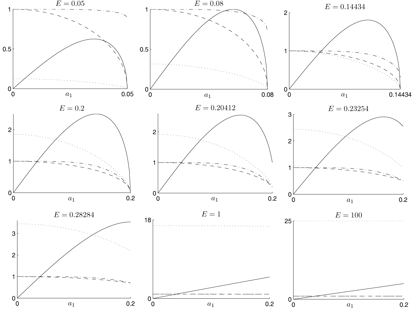
Figure 8: Moduli of kinematic (dashed), Fermi (solid), spectroscopic (dot-dashed) and astrometric (dotted) relative velocities with $a_{2}=0.2$. At $E=0.08$ (top center), $\left\|v_{\mathrm{Fermi}}\right\|_{\mathrm{max}}$ begins to be superluminal. At $E=0.14434$ (top right), $\left\|v_{\mathrm{ast}}\right\|_{\mathrm{sup}}$ begins to be superluminal. At $E=a_{2}=0.2$ (middle left), all the velocities vanish at $a_{1}=a_{1\mathrm{max}}=0.2$, and these minima begin to increase for higher energies. At $E=0.20412$ (middle center), the relative minimum of $\left\|v_{\mathrm{Fermi}}\right\|$ at $a_{1}=0.2$ begins to be superluminal. At $E=0.23254$ (middle right), $\left\|v_{\mathrm{ast}}\right\|_{\mathrm{min}}$ begins to be superluminal. At $E=0.28284$ (bottom left), $\left\|v_{\mathrm{Fermi}}\right\|$ begins to be monotonic.

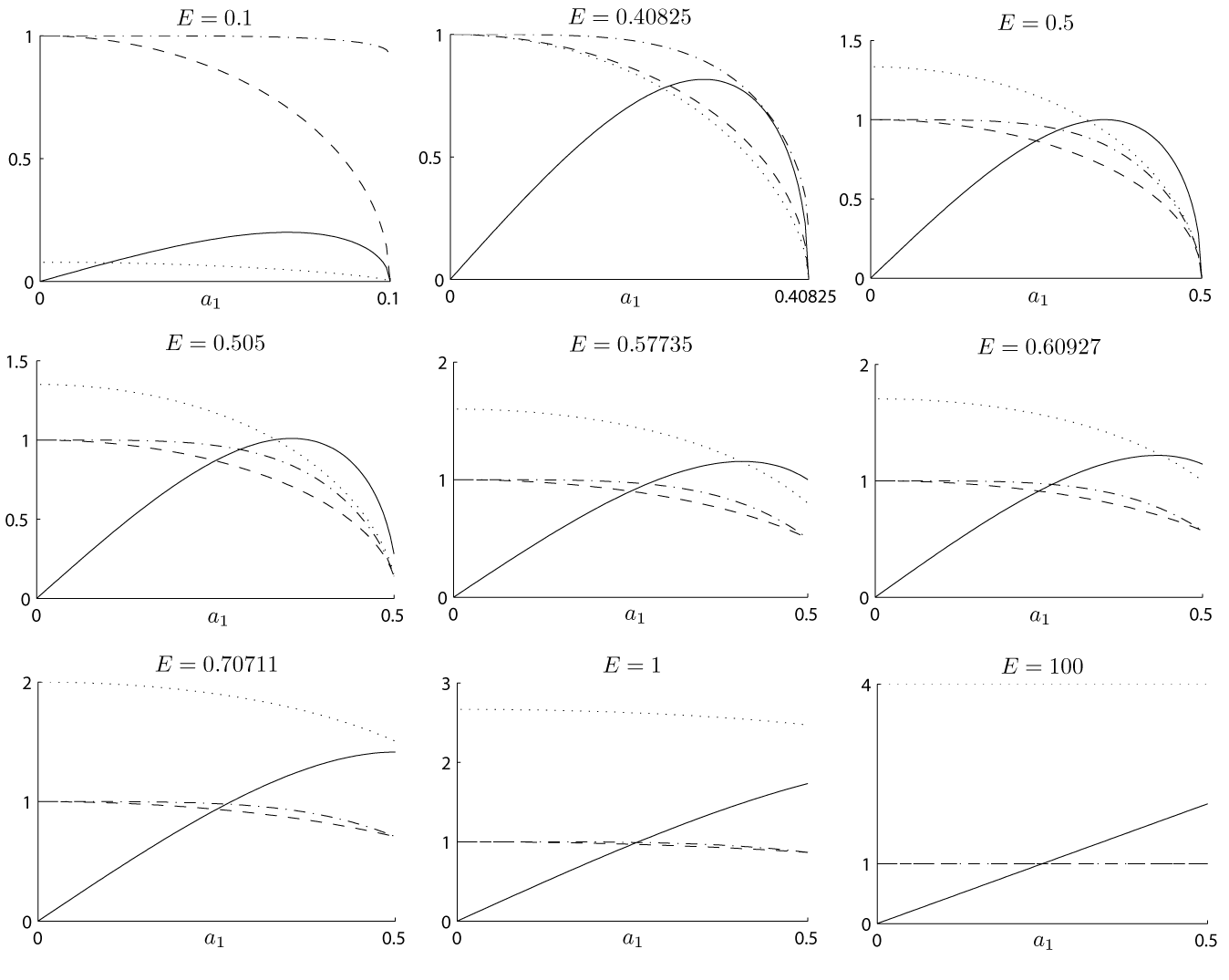
Figure 9: Moduli of kinematic (dashed), Fermi (solid), spectroscopic (dot-dashed) and astrometric (dotted) relative velocities with $a_{2}=0.5$. At $E=0.40825$ (top center), $\left\|v_{\mathrm{ast}}\right\|_{\mathrm{sup}}$ begins to be superluminal. At $E=a_{2}=0.5$ (top right), all the velocities vanish at $a_{1}=a_{1\mathrm{max}}=0.5$, and these minima begin to increase for higher energies; moreover $\left\|v_{\mathrm{Fermi}}\right\|_{\mathrm{max}}$ begins to be superluminal. At $E=0.57735$ (middle center), the relative minimum of $\left\|v_{\mathrm{Fermi}}\right\|$ at $a_{1}=0.5$ begins to be superluminal. At $E=0.60927$ (middle right), $\left\|v_{\mathrm{ast}}\right\|_{\mathrm{min}}$ begins to be superluminal. At $E=0.70711$ (bottom left), $\left\|v_{\mathrm{Fermi}}\right\|$ begins to be monotonic.

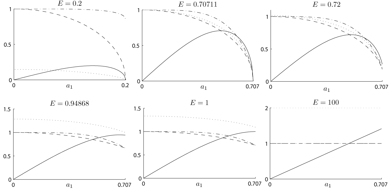
Figure 10: Moduli of kinematic (dashed), Fermi (solid), spectroscopic (dot-dashed) and astrometric (dotted) relative velocities with $a_{2}=0.70711$ $(r_{2}=4m)$. At $E=a_{2}=0.70711$ (top center), all the velocities vanish at $a_{1}=a_{1\mathrm{max}}=0.70711$, and these minima begin to increase for higher energies; moreover $\left\|v_{\mathrm{ast}}\right\|_{\mathrm{sup}}$ begins to be superluminal. At $E=0.94868$ (bottom left), $\left\|v_{\mathrm{ast}}\right\|_{\mathrm{min}}$ begins to be superluminal. At $E=1$ (bottom center), $\left\|v_{\mathrm{Fermi}}\right\|$ begins to be monotonic and its maximum at $a_{1}=0.70711$ begins to be superluminal.

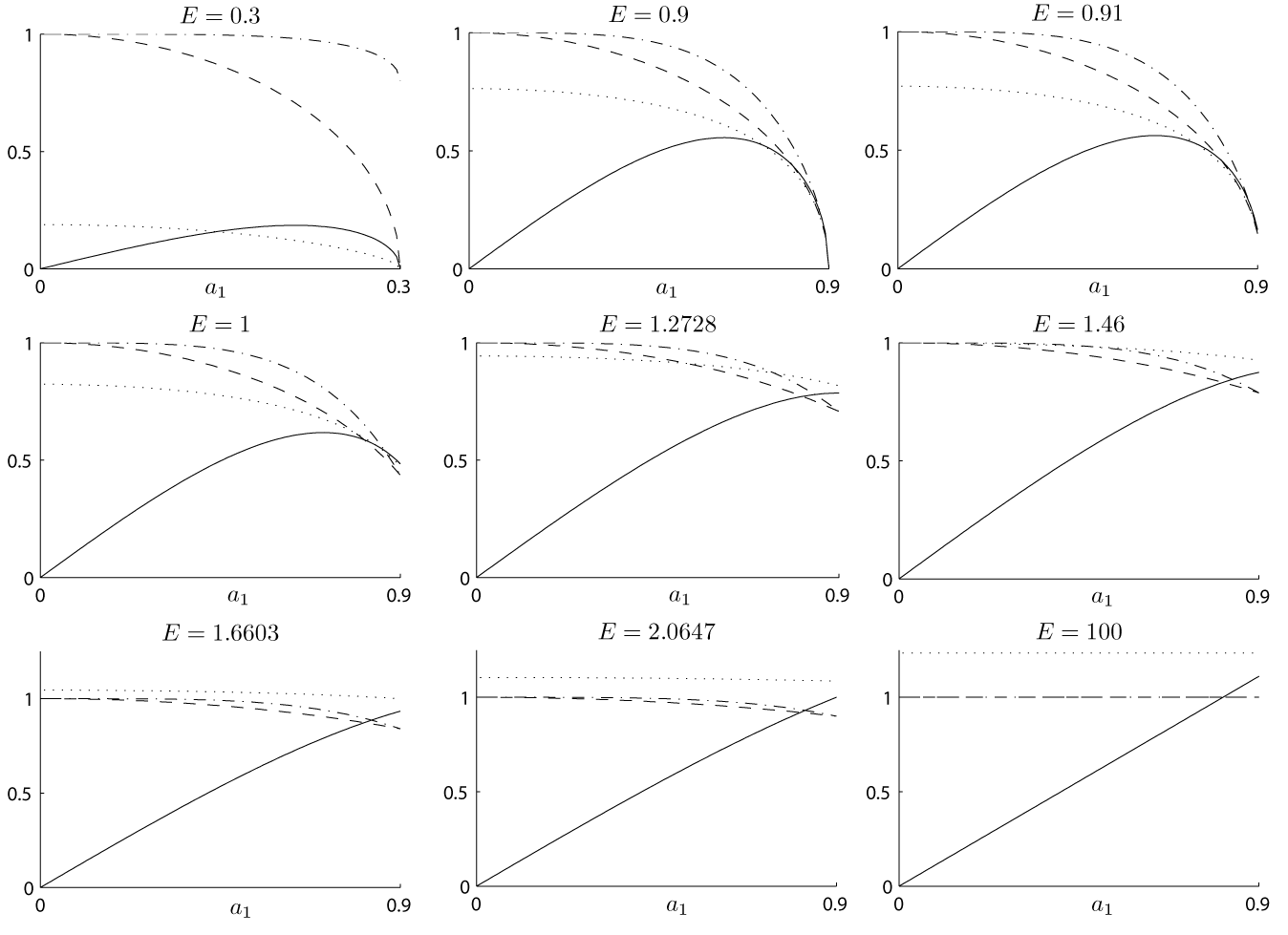
Figure 11: Moduli of kinematic (dashed), Fermi (solid), spectroscopic (dot-dashed) and astrometric (dotted) relative velocities with $a_{2}=0.9$. At $E=a_{2}=0.9$ (top center), all the velocities vanish at $a_{1}=a_{1\mathrm{max}}=0.9$, and these minima begin to increase for higher energies. At $E=1.2728$ (middle center), $\left\|v_{\mathrm{Fermi}}\right\|$ begins to be monotonic. At $E=1.46$ (middle right), $\left\|v_{\mathrm{ast}}\right\|_{\mathrm{sup}}$ begins to be superluminal. At $E=1.6603$ (bottom left), $\left\|v_{\mathrm{ast}}\right\|_{\mathrm{min}}$ begins to be superluminal. At $E=2.0647$ (bottom center), $\left\|v_{\mathrm{Fermi}}\right\|_{\mathrm{max}}$ begins to be superluminal.

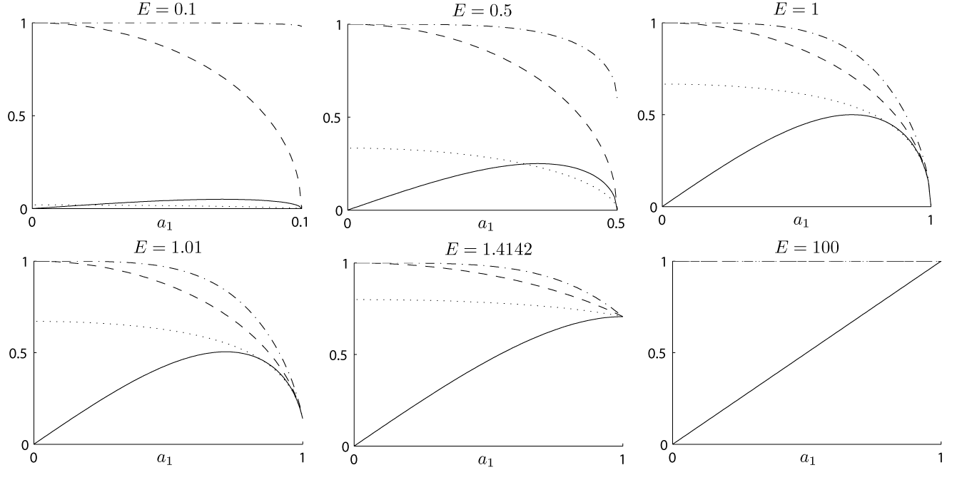
Figure 12: Moduli of kinematic (dashed), Fermi (solid), spectroscopic (dot-dashed) and astrometric (dotted) relative velocities in the exterior limit $a_{2}=1$. There is not any superluminal velocity. At $E=a_{2}=1$ (top right), all the velocities vanish at $a_{1}=a_{1\mathrm{max}}=1$, and this minimum (note that all the velocities have the same minimum) begins to increase for higher energies. At $E=\sqrt{2}$ (bottom center), $\left\|v_{\mathrm{Fermi}}\right\|$ begins to be monotonic.

References

- [1] M. Soffel, et al. The IAU 2000 resolutions for astrometry, celestial mechanics and metrology in the relativistic framework: explanatory supplement. Astron. J. 126 (2003), 2687–2706 (arXiv:astro-ph/0303376).
- [2] L. Lindegren, D. Dravins. The fundamental definition of ‘radial velocity’. Astron. Astrophys. 401 (2003), 1185–1202 (arXiv:astro-ph/0302522).
- [3] S. Helgason. Differential Geometry and Symmetric Spaces. Academic Press, London (1962).
- [4] E. Fermi. Sopra i fenomeni che avvengono in vicinanza di una linea oraria. Atti R. Accad. Naz. Lincei, Rendiconti, Cl. sci. fis. mat & nat. 31 (1922), 21–23, 51–52, 101–103.
- [5] K. P. Marzlin. On the physical meaning of Fermi coordinates. Gen. Relativity Gravitation 26 (1994), 619–636 (arXiv:gr-qc/9402010).
- [6] D. Bini, L. Lusanna, B. Mashhoon. Limitations of radar coordinates. Int. J. Mod. Phys. D 14 (2005), 1413–1429 (arXiv:gr-qc/0409052).
- [7] J. Olivert. On the local simultaneity in general relativity. J. Math. Phys. 21 (1980), 1783–1785.
- [8] V. J. Bolós, V. Liern, J. Olivert. Relativistic simultaneity and causality. Internat. J. Theoret. Phys. 41 (2002), no. 6, 1007–1018 (arXiv:gr-qc/0503034).
- [9] G. F. R. Ellis, S. D. Nel, R. Maartens, W. R. Stoeger, A. P. Whitman. Ideal observational cosmology. Phys. Rep. 124 (1985), no. 5-6, 315–417.
- [10] J. K. Beem, P. E. Ehrlich. Global Lorentzian Geometry. Marcel Dekker, New York (1981).
- [11] R. K. Sachs, H. Wu. Relativity for Mathematicians. Springer Verlag, Berlin, Heidelberg, New York (1977).
- [12] V. J. Bolós. Lightlike simultaneity, comoving observers and distances in general relativity. J. Geom. Phys. 56 (2006), no. 5, 813–829 (arXiv:gr-qc/0501085).
- [13] W. O. Kermack, W. H. McCrea, E. T. Whittacker. On properties of null geodesics and their application to the theory of radiation. Proc. R. Soc. Edinburgh 53 (1932), 31–47.
- [14] D. Klein, P. Collas. Recessional velocities and Hubble’s law in Schwarzschild-de Sitter space. Phys. Rev. D 81 (2010), 063518 (arXiv:1001.1875).
- [15] P. Crawford, I. Tereno. Generalized observers and velocity measurements in general relativity. Gen. Relativity Gravitation 34 (2002), no. 12, 2075–2088 (arXiv:gr-qc/0111073).
- [16] D. Klein, E. Randles. Fermi coordinates, simultaneity, and expanding space in Robertson-Walker cosmologies. Ann. Henri Poincaré 12 (2011), 303–328 (arXiv:1010.0588).
- [17] W. Misner, K. Thorne, J. Wheeler. Gravitation. Freeman, New York (1973).