Quasinormal modes of Rarita-Schwinger field in Reissner-Nordström black hole spacetimes

Abstract

The Newman-Penrose formalism is used to deal with the quasinormal modes(QNM’s) of Rarita-Schwinger perturbations outside a Reissner-Nordström black hole. We obtain four kinds of possible expressions of effective potentials, which are proved to be of the same spectra of quasinormal mode frequencies. The quasinormal mode frequencies evaluated by the WKB potential approximation show that, similar to those for Dirac perturbations, the real parts of the frequencies increase with the charge $Q$ and decrease with the mode number $n$, while the dampings almost keep unchanged as the charge increases.
PACS: number(s): 04.70.Dy, 04.70.Bw, 97.60.Lf
Keywords: Black hole, QNM’s, Rarita-Schwinger field, Reissner-Nordström, WKB approximation.

For several decades, the QNM’s of black holes have been of great interest both to gravitation theorists and to gravitational-wave experimentalists [1, 2, 3] due to the remarkable fact that QNM’s allow us not only to test the stability of the event horizon against small perturbations, but also to probe the parameters of black hole, such as its mass, electric charge, and angular momentum. QNM’s are induced by the external perturbations. For instance, if an unfortunate astronaut fall into a black hole, the surrounding geometry will undergo damped oscillations. They can be accurately described in terms of a set of discrete spectrum of complex frequencies, whose real parts determine the oscillation frequency, and whose imaginary parts determine the damped rate. Mathematically, they are defined as solutions of the perturbation equations belonging to certain complex characteristic frequencies which satisfy the boundary conditions appropriate for purely ingoing waves at the event horizon and purely outgoing waves at infinity[4].
   Recent observational results suggest that our Universe in large scale is described by Einstein equations with a cosmology constant. Motivated by the recent anti-de Sitter (AdS) conformal field theory (CFT) correspondence conjecture[5], much attention has been paid to the QNM’s in AdS spacetimes[2, 3]. The latest studies on quantum gravity show that QNM’s also play an important role in this realm due to their close relations to the Barbero-Immirzi parameter, a factor introduced by hand in order that loop quantum gravity reproduces correctly entropy of the black hole[6, 7, 8, 9].
    A well-known fact is that quasinormal mode (QN) frequencies are closely related to the spin of the exterior perturbation fields[10]. Previous works on QNM’s in black holes has concentrated on the perturbation for scalar, neutrino, electromagnetic and gravitational fields[3]. However, few has been done for the case of Rarita-Schwinger fields, which closely relate to supergravity. According to the supergravity theory, the Rarita-Schwinger field acts as a source of torsion and curvature, the supergravity field equations reduce to Einstein vacuum field equations when Rarita-Schwinger field vanishes. This can be seen from the action of supergravity, namely[11],

$$I=\int d^{4}x(\textit{L}_{2}+\textit{L}_{3/2}),$$

where $\textit{L}_{2}$ and $\textit{L}_{3/2}$ represent the Lagrangian of gravitational and Rarita-Schwinger fields, respectively. We hence expect to obtain some interesting and new physics by investigating ONM’s of Rarita-Schwinger field.
    As to QNM’s, the first step is to obtain the one-dimensional radial wave-equation. We usually start with linearized perturbation equations. Two often used ways are available for obtaining the linearized perturbation equations. One is a straightforward but usually complicated way that linearize the Rarita-Schwinger equation directly and deduce a set of partial differential equations (one can see Ref.[12] for details); The other is provided by the Newman-Penrose (N-P) formalism, which end up with partial differential equations in $r$ and $\theta$ instead of ordinary differential equations in $r$. Torres[13] have deduced the linearized Rarita-Schwinger equation in N-P formalism for a type D vacuum background. We start with the Rarita-Schwinger equation in a curved background space-time

$$\nabla_{A\dot{D}}\psi^{A}_{B\dot{C}}=\nabla_{B\dot{C}}\psi^{A}_{A\dot{D}}.$$ (1)

or, in the Newman-Penrose notation, namely, the Teukolsky’s master equations[14, 15]

$$\{[D-2\epsilon+\epsilon^{*}-3\rho-\rho^{*}](\bar{\Delta}-3\gamma+\mu)$$

$$-[\delta-2\beta-\alpha^{*}-3\tau+\pi^{*}](\bar{\delta}-3\alpha+\pi)-\Psi_{2}\}\Phi_{3/2}=0,$$ (2)

and

$$\{[\bar{\Delta}+2\gamma-\gamma^{*}+3\mu+\mu^{*}](D+3\epsilon-\rho)$$

$$-[\bar{\delta}+2\alpha+\beta^{*}+3\pi-\tau^{*}](\delta+3\beta-\tau)-\Psi_{2}\}\Phi_{-3/2}=0.$$ (3)

Here we have introduced a null tetrad $(l^{\mu},n^{\mu},m^{\mu},\bar{m}^{\mu})$ which satisfies the orthogonality relations $l_{\mu}n^{\mu}=-m_{\mu}\bar{m}^{\mu}=1$ and $l_{\mu}m^{\mu}=l_{\mu}\bar{m}^{\mu}=n_{\mu}m^{\mu}=n_{\mu}\bar{m}^{\mu}=0$, and the metric conditions $g_{\mu\nu}=l_{\mu}n_{\nu}+n_{\mu}l_{\nu}-m_{\mu}\bar{m}_{\nu}-\bar{m}_{\mu}m_{\nu}$. According to these conditions, we can take the null tetrad as $l^{\mu}=(e^{-2U(r)},1,0,0)$, $n^{\mu}=\frac{1}{2}(1,-e^{2U(r)},0,0)$, $m^{\mu}=\frac{1}{\sqrt{2}r}\left(0,0,1,\frac{i}{\sin\theta}\right)$, $\bar{m}^{\mu}=\frac{1}{\sqrt{2}r}\left(0,0,1,-\frac{i}{\sin\theta}\right).$ The corresponding covariant null tetrad is $l_{\mu}=(1,-e^{-2U(r)},0,0)$, $n_{\mu}=\frac{1}{2}(e^{2U(r)},1,0,0)$ , $m_{\mu}=-\frac{r}{\sqrt{2}}\left(0,0,1,i\sin\theta\right)$, $\bar{m}_{\mu}=-\frac{r}{\sqrt{2}}\left(0,0,1,-i\sin\theta\right)$. The non-vanishing spin coefficients read

$$\rho=-\frac{1}{r},\quad\alpha=-\beta=-\frac{\cot\theta}{2\sqrt{2}r},\quad\mu=-\frac{e^{2U(r)}}{2r},\quad\gamma=\frac{1}{4}(e^{2U(r)})^{\prime},$$ (4)

and only one of Weyl tensors is not zero, i.e., $\Psi_{2}=-\frac{(e^{2U(r)})^{\prime}}{2r}$, where a prime denotes the partial differential with respect to $r$.
   In standard coordinates, the line element for the Reissner-Nordström spacetime can be expressed as

$$ds^{2}=-e^{2U(r)}dt^{2}+e^{-2U(r)}dr^{2}+r^{2}\left({d\theta^{2}+sin^{2}\theta d\varphi^{2}}\right),$$ (5)

with

$$e^{2U(r)}=1-\frac{{2M}}{{r}}+\frac{Q^{2}}{r^{2}},$$ (6)

where $M$ and $Q$ are the mass and charge of the black hole, respectively.
   The directional derivatives given in Eqs.(2) and (3), when applied as derivatives to the functions with a $t$- and a $\varphi$-dependence specified in the form $e^{i(\omega t+m\varphi)}$, become the derivative operators

$$D=\mathscr{D}_{0},\quad\bar{\Delta}=-\frac{\Delta}{2r^{2}}\mathscr{D}^{{\dagger}}_{0},\quad\delta=\frac{1}{\sqrt{2}r}\mathscr{L}^{{\dagger}}_{0},\quad\bar{\delta}=\frac{1}{\sqrt{2}r}\mathscr{L}_{0},$$ (7)

where

$$\mathscr{D}_{n} = \partial_{r}+\frac{i\omega r^{2}}{\Delta}+n\cdot\frac{\Delta^{\prime}}{\Delta},\quad\mathscr{D}^{{\dagger}}_{n}=\partial_{r}-\frac{i\omega r^{2}}{\Delta}+n\cdot\frac{\Delta^{\prime}}{\Delta},$$

$$\mathscr{L}_{n} = \partial_{\theta}+\frac{m}{\sin\theta}+n\cot\theta,\quad\mathscr{L}^{{\dagger}}_{n}=\partial_{\theta}-\frac{m}{\sin\theta}+n\cot\theta,$$ (8)

and

$$\Delta=r^{2}-2Mr+Q^{2}.$$ (9)

It is obvious that $\mathscr{D}_{n}$ and $\mathscr{D}^{{\dagger}}_{n}$ are purely radial operators, while $\mathscr{L}_{n}$ and $\mathscr{L}^{{\dagger}}_{n}$ are purely angular operators. After some transformations are made, Eqs.(2) and (3) can be decoupled as the two pairs of equations[10],

$$[\Delta\mathscr{D}_{-1/2}\mathscr{D}^{{\dagger}}_{0}-4i\omega r]P_{+3/2} = \lambda P_{+3/2},$$ (10)

$$\mathscr{L}^{{\dagger}}_{-1/2}\mathscr{L}_{3/2}A_{+3/2} = -\lambda A_{+3/2},$$ (11)

and

$$[\Delta\mathscr{D}^{{\dagger}}_{-1/2}\mathscr{D}_{0}+4i\omega r]P_{-3/2} = \lambda P_{-3/2},$$ (12)

$$\mathscr{L}_{-1/2}\mathscr{L}^{{\dagger}}_{3/2}A_{-3/2} = -\lambda A_{-3/2},$$ (13)

where $\lambda$ is a separation constant. The reason we have not distinguished the separation constants in Eqs.(11)- (13) is that $\lambda$ is a parameter that is to be determined by the fact that $A_{+3/2}$ should be regular at $\theta=0$ and $\theta=\pi$, and thus the operator acting on $A_{-3/2}$ on the left-hand side of Eq.(13) is the same as the one on $A_{+3/2}$ in Eq.(11) if we replace $\theta$ by $\pi-\theta$.
In Reissner-Nordström black hole, the separation constant can be determined analytically[15, 16, 17]

$$\lambda=\begin{cases}(l+3)(l+1)\quad\quad\quad&\text{for}\quad j=l+s,\\ l(l-2)\quad\quad\quad&\text{for}\quad j=l-s,\end{cases}$$ (14)

where $l=2,3,4,\cdots$. Note we only consider the case for $j=l+s$ in our following discussions, the case for $j=l-s$ can be easily obtained in the same way. Since $P_{+3/2}$ and $P_{-3/2}$ satisfy complex-conjugate equations (10) and (12), it will suffice to consider the equation (10) only.
   By introducing a tortoise coordinate transformation $dr_{*}=\frac{r^{2}}{\Delta}dr$, and defining $\Lambda_{\pm}=\frac{d}{dr_{*}}\pm i\omega$, $Y=r^{-2}P_{+3/2}$, one can rewrite Eq.(10) in a simplified form

$$\Lambda^{2}Y+\tilde{P}\Lambda_{-}Y-\tilde{Q}Y=0,$$ (15)

where

$$\tilde{P}=\frac{d}{dr_{*}}\ln\frac{r^{6}}{\Delta^{3/2}},\quad\tilde{Q}=\frac{\Delta}{r^{4}}\left[\lambda-(\frac{2\Delta}{r^{2}}-\frac{\Delta^{\prime}}{r})\right].$$ (16)

Transformation theory [4] shows that one can transform Eq.(15) to a one-dimensional wave-equation of the form $\Lambda^{2}Z=VZ$ by introducing some parameters (certain functions of $r_{*}$ to be determined) $\xi(r_{*})$, $\chi(r_{*})$, $\beta_{1}(r_{*})$, $T_{1}(r_{*})$, and several constants (to be specified) $\beta_{2}$, $T_{2}$, $\kappa$, $\kappa_{1}$. If we assume that $Y$ is related to $Z$ in the manner $Y=\xi VZ+T\Lambda_{+}Z$, and the relations $T=T_{1}(r_{*})+2i\omega,\beta=\beta_{1}(r_{*})+2i\omega\beta_{2}$, one can obtain a equation governing $\beta_{2}$, $\kappa$, $\kappa_{1}$ derived from eq.(15)[10]

$$\frac{\Delta^{3/2}}{r^{6}}(F+\beta_{2})^{2}-\frac{(F+\beta_{2})F_{,r_{*},r_{*}}}{F-\beta_{2}}+\frac{({F_{,r_{*}}}^{2}-\kappa_{1}^{2})F}{(F-\beta_{2})^{2}}=\kappa,$$ (17)

where we have defined $F=\frac{r^{6}\tilde{Q}}{\Delta^{3/2}}$, and ‘$,r_{*}$’ denotes the differential with respect to $r_{*}$. A key step to obtain the expression of potential $V$ is to seek available $\beta_{2}$, $\kappa$, and $\kappa_{1}$ whose values satisfy Eq.(17). Further study shows that $F$ as defined in the previous text does satisfy Eq.(17) with the choice

$$\beta_{2}=\pm 2Q,\quad\kappa=0,\quad\kappa_{1}=\pm\lambda\sqrt{1+\lambda}.$$ (18)

The potential $V$ can then be expressed as

$$V=-\frac{\Delta^{3/2}}{r^{6}}\beta_{2}-\frac{(F_{,r_{*}}-\kappa_{1})(\kappa_{1}F-\beta_{2}F_{,r_{*}})}{(F-\beta_{2})(F^{2}-\beta_{2}^{2})},$$ (19)

Note that the sign of $\beta_{2}$ and $\kappa_{1}$ can be assigned independently, so there exists four sets of expressions of $V$. Here we denote them by $V^{j}(j=1,2,3,4)$. Chandrasekhar pointed out that there has a closed relation between the solutions belonging to the different potentials showed in equation(19) (see Ref.[4] §97(d) for details)

$$K^{i}Z^{i}=\left\{\frac{F+\beta_{2}^{i}}{F+\beta_{2}^{j}}K^{j}+\left[i\omega\frac{F-\beta_{2}^{j}}{F+\beta_{2}^{j}}-\frac{\kappa_{1}^{j}F-\beta_{2}^{j}F^{\prime}}{F^{2}-\beta_{2}^{2}}\right]D^{ij}\right\}Z^{j}+D^{ij}\frac{dZ^{j}}{dr_{*}},$$ (20)

where

$$K = -4\omega^{2}\beta_{2}+2i\omega\kappa_{1},$$ (21)

$$D^{ij} = 2i\omega(\beta_{2}^{i}-\beta_{2}^{j})+(\kappa_{1}^{i}-\kappa_{1}^{j})\frac{F^{2}-\beta_{2}^{2}}{(F-\beta_{2}^{i})(F-\beta_{2}^{j})}$$ (22)

One can easily prove that the potentials vanish when we let $r\rightarrow\pm\infty$

$$V^{j} \to e^{\frac{r_{*}}{2M}}, r_{*}\to-\infty$$ as ,

$$V^{j} \to r^{-2}, r_{*}\to+\infty$$ as .

A direct consequence of this property is that the wave-function has an asymptotically flat behavior for $r\rightarrow\pm\infty$, i.e., $Z\rightarrow e^{\mp i\omega r_{*}}$ (this is just the boundary conditions of QNM’s). It has shown that in asymptotically flat spacetimes, solutions related in the way showed in Eq.(20) yield the same reflexion and transmission coefficients, and hence possess the same spectra of QN frequencies[4]. Moreover, we can easily obtain the potentials for negative charge by rearranging the order of $V^{j}$ for positive ones since $\beta_{2}$ equals to $\pm 2Q$. Therefore, we shall concentrate just on potential with $\beta_{2}=2Q(Q>0,say)$ and $\kappa_{1}=\lambda\sqrt{1+\lambda}$ in our following works.
   We hence know that the radial equation (10) can be simplified to a one-dimensional wave-equation of the form

$$\frac{d^{2}Z}{dr_{*}^{2}}+\omega^{2}Z=VZ,$$ (23)

where

$$V=-\frac{2Q\Delta^{3/2}}{r^{6}}-\frac{(F_{,r_{*}}-\lambda\sqrt{1+\lambda})(\lambda\sqrt{1+\lambda}F-2QF_{,r_{*}})}{(F-2Q)(F^{2}-4Q^{2})}.$$ (24)

Note that we have written $V^{j}$ as $V$ because we only work with one case of the potentials.
   The effective potential $V(r,Q,l)$, which depends only on the value of $r$ for fixed $Q$ and $l$, has a maximum over $r\in(r_{+},+\infty)$. The location $r_{0}$ of the maximum has to be evaluated numerically. An interesting phenomenon is that the position of the potential peak approaches a critical value when $l\rightarrow\infty$, i.e.,

$$r_{0}(l\rightarrow\infty)\rightarrow 3M.$$ (25)

Obviously, the effective potential relates to the electric charge of black hole. Figure 1 demonstrates the variation of the effective potential $V(r,Q,l)$ with respect to charge $Q$ for fixed $l=2$. From this we can see that the peak value of the effective potential $V$ increases with $Q$, but the location of the peak decreases with charge. This is quite consistent with the case for Dirac perturbation in Reissner-Nordström black hole spacetimes.

2.5in

Figure 1: Variation of the effective potential for massless gravitino with $M=1$, $l=2$, $Q=0,0.3,0.6,0.9$

We now evaluate their frequencies by using third-order WKB potential approximation[10], a numerical method devised by Schutz and Will[18], and was extended to higher orders in[19, 20]. Due to its considerable accuracy for lower-lying modes[21], this analytic method has been used widely in evaluating QN frequencies of black holes. Noting that during our evaluating procedures, we have let the mass $M$ of the black hole as a unit of mass so as to simplify the calculation. The values are listed in Table 1, where we only list the values for $l=5$ as an example. Values for other mode numbers can easily obtained in the same way. As a reference, we have also evaluated the values (listed in Table 2) for $l=5$ by using the first-order WKB potential approximation[18]. Obviously, compared to the first-order approximation, great improvement, especially for larger $n$, has been made for third-order approximation.
    Figure 2 demonstrates the variation of real and imaginary part of the QN frequencies with different $Q$ and $n$ for $l=5$. It shows that the real part of the quasinormal mode frequencies increases with the charge $Q$, while decreases with $n$. But things are totally different for the imaginary part as showed in the figure, whose values almost keep unchanged as the charge increasing, whereas them increase very quickly with the mode number. Furthermore, there is also an interesting phenomena that the larger the charge is, the smaller effect of $n$ on the real part of QN frequencies may have.

Table 1: QN frequencies of Rarita-Schwinger field in RN black hole for $l=5$ (third-order WKB approximation)

$Q$	$n=0$	$n=1$	$n=2$	$n=3$	$n=4$
0	1.3273+0.0958i	1.3196+0.2881i	1.3048+0.4824i	1.2839+0.6795i	1.2582+0.8794i
0.1	1.3295+0.0959i	1.3218+0.2883i	1.3070+0.4827i	1.2863+0.6798i	1.2606+0.8799i
0.2	1.3364+0.0960i	1.3287+0.2888i	1.3140+0.4835i	1.2933+0.6809i	1.2678+0.8813i
0.3	1.3481+0.0963i	1.3405+0.2895i	1.3260+0.4847i	1.3055+0.6826i	1.2802+0.8834i
0.4	1.3653+0.0966i	1.3579+0.2906i	1.3436+0.4864i	1.3234+0.6849i	1.2985+0.8863i
0.5	1.3890+0.0970i	1.3817+0.2918i	1.3677+0.4884i	1.3481+0.6876i	1.3238+0.8896i
0.6	1.4206+0.0974i	1.4136+0.2930i	1.4001+0.4903i	1.3811+0.6902i	1.3576+0.8928i
0.7	1.4627+0.0977i	1.4560+0.2938i	1.4432+0.4916i	1.4251+0.6917i	1.4027+0.8945i
0.8	1.5197+0.0976i	1.5135+0.2932i	1.5016+0.4904i	1.4848+0.6898i	1.4639+0.8916i

Table 2: QN frequencies of Rarita-Schwinger field in RN black hole for $l=5$ (first-order WKB approximation)

$Q$	$n=0$	$n=1$	$n=2$	$n=3$	$n=4$
0	1.3358+0.0957i	1.3618+0.2817i	1.4077+0.4542i	1.4657+0.6108i	1.5300+0.7522i
0.1	1.3380+0.0958i	1.3640+0.2819i	1.4099+0.4545i	1.4679+0.6112i	1.5323+0.7528i
0.2	1.3448+0.0959i	1.3708+0.2824i	1.4166+0.4554i	1.4747+0.6125i	1.5391+0.7546i
0.3	1.3566+0.0962i	1.3825+0.2832i	1.4282+0.4569i	1.4862+0.6147i	1.5507+0.7575i
0.4	1.3737+0.0966i	1.3995+0.2843i	1.4451+0.4589i	1.5031+0.6177i	1.5677+0.7615i
0.5	1.3973+0.0970i	1.4229+0.2857i	1.4683+0.4614i	1.5262+0.6215i	1.5908+0.7666i
0.6	1.4288+0.0974i	1.4541+0.2871i	1.4991+0.4641i	1.5567+0.6257i	1.6213+0.7724i
0.7	1.4707+0.0977i	1.4954+0.2882i	1.5398+0.4664i	1.5968+0.6297i	1.6610+0.7783i
0.8	1.5273+0.0975i	1.5512+0.2880i	1.5942+0.4671i	1.6500+0.6318i	1.7133+0.7823i

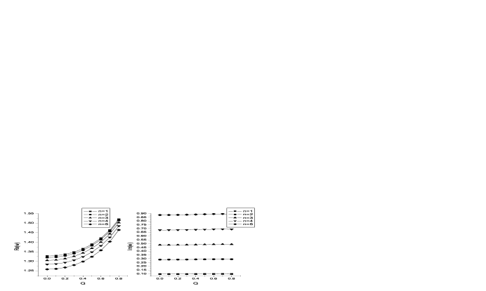
Figure 2: Variation of the QN frequencies for $V$ with different $Q$ and $n$ for $l=5$.

Acknowledgements

One of the authors(Fu-wen Shu) wishes to thank Doctor Xian-Hui Ge for his valuable discussion. The work was supported by the National Natural Science Foundation of China under Grant No. 10273017.

References

- [1] V.Cardoso, and J.P.S.Lemos, Phys.Rev.D 63, 124015(2001); C.Molina, Phys.Rev.D 68, 064007(2003); F.W.Shu, and Y.G.Shen Phys.Rev.D 70, 084046(2004); I.G.Moss, and J.P.Norman Class.Quantum Grav. 19, 2323(2002); E.Berti, V.Cardoso, and S.Yoshida Phys.Rev.D 69, 124018(2004).
- [2] G.T.Horowitz, and V.Hubeny, Phys.Rev.D 62, 024027(2000).
- [3] V.Cardoso, and J.P.S.Lemos, Phys.Rev.D 64, 084017(2001);
- [4] S.Chandraskhar, The Mathematical Theory of Black Holes (Oxford University Press, Oxford, England, 1983).
- [5] J.Maldacena, Adv.Theor.Math.Phys. 2, 253(1998).
- [6] S.Hod, Phys. Rev. Lett. 81, 4293(1998).
- [7] O.Dreyer, Phys. Rev. Lett. 90, 081301(2003).
- [8] A.Corichi, Phys.Rev.D 67, 087502(2003).
- [9] J.Bekenstein, Lett.Nuovo Cimento Soc.Ital.Fis. 11, 467(1974); J.Bekenstein, in Cosmology and Gravitation, edited by M.Novello (Atlasciences, France, 2000), pp. 1-85, gr-qc/9808028; J.Bekenstein and V.F.Mukhanov, Phys.Lett.B 360, 7(1995).
- [10] F.W.Shu, and Y.G.Shen, gr-qc/0501098.
- [11] D.Z.Freedman, P.V.Nieuwenhuizen, and S.FerraraPhys.Rev.D 13, 3214(1976).
- [12] C.V.Vishveshwara, Nature, 227,936(1970); F.J.Zerrili, Phys.Rev.D 2, 2141(1970).
- [13] G.F.Torres del Castillo, J.Math.Phys. 30, 446(1989).
- [14] S.A.Teukolsky, Phys.Rev.Lett. 29, 1114(1972); Astrophys.J. 185, 635(1973); S.A.Teukolsky and W.H.Press, ibid. 193, 443(1974);
- [15] W.H.Press and S.A.Teukolsky, ibid.185, 649(1973).
- [16] E.T.Newman, and R.Penrose, J.Math.Phys. 3, 556(1962).
- [17] E.T.Newman, and R.Penrose, ibid. 7, 863(1966); J.N.Goldberg, A.J.Macfarlane, E.T.Newman, F.Rohrlich, and E.C.G.Sudarshan, J.Math.Phys. 8, 2155(1967).
- [18] B.F.Schutz, and C.M.Will, Astrophys.J.Lett.Ed. 291, L33(1985).
- [19] S.Iyer and C.M.Will, Phys.Rev.D 35, 3621(1987).
- [20] R.A.Konoplya, Phys.Rev.D 68, 024018(2003).
- [21] S.Iyer, Phys.Rev.D 35, 3632(1987).