Using the inspiral program to search for gravitational waves from low-mass binary inspiral

Abstract

The inspiral program is the LIGO Scientific Collaboration’s computational engine for the search for gravitational waves from binary neutron stars and sub-solar mass black holes. We describe how this program, which makes use of the findchirp algorithm (discussed in a companion paper), is integrated into a sophisticated data analysis pipeline that was used in the search for low-mass binary inspirals in data taken during the second LIGO science run.

1 Introduction

The search for gravitational waves that arise from coalescing compact binary systems—binary neutron stars and black holes—is one of the main efforts in LIGO data analysis conducted by the LIGO Scientific Collaboration (LSC). For the first science run of LIGO, we focused attention on the search for low-mass binary systems (binary neutron stars and sub-solar mass binary black hole systems) since these systems have well-understood waveforms [1]. For the second science run of LIGO, S2, we have extended our analysis to include searches for binary black hole systems with higher masses. This work will be described elsewhere [2]. Here we describe the refinements to the original S1 search for low-mass binary inspiral waveforms: binary neutron star systems [3] and sub-solar-mass binary black hole systems which may be components of the Milky Way Halo (and thus form part of a hypothetical population of Macroscopic Astrophysical Compact Halo Objects known as MACHOs) [4]. In this paper we focus on how the central computational search engine—the inspiral program—is integrated into a sophisticated new data analysis pipeline that was used in the S2 low-mass binary inspiral search.

The inspiral program makes use of the LSC inspiral search algorithm findchirp, which is described in detail in a companion paper [5]. This companion paper describes the algorithm that we use to generate inspiral triggers given an inspiral template and a single data segment. There is more to searching for gravitational waves from binary inspiral than trigger generation, however. To perform a search for a given class of sources in a large quantity of interferometer data we construct a detection pipeline.

The detection pipeline is divided into blocks that perform specific tasks. These tasks are implemented as individual programs. The pipeline itself is then implemented as a logical graph, called a directed acyclic graph or DAG, describing the workflow (the order that the programs must be called to perform the pipeline activities) which can then be submitted to a batch processing system on a computer cluster. We use the Condor high throughput computing system [6] to manage the DAG and to control the execution of the programs.

The structure of this paper will follow these various tasks (programs). In Sec. 2 we provide an overview of these tasks and then describe each task in turn. In Sec. 3 we provide a simple illustration of how these elements are combined into a workflow pipeline.

2 Pipeline overview

In LIGO’s second science run S2 we performed a triggered search for low-mass binary inspirals: since we require that a trigger occur simultaneously and consistently in at least two detectors located at different sites in order for it to be considered as a detection candidate, we save computational effort by analyzing data from the Livingston interferometer first and then performing follow-up analyses of Hanford data only for the specific triggers found. We describe the tasks and their order of execution in this triggered search as our detection pipeline.

An overview of the tasks required in the detection pipeline are: (i) data selection with the datafind program, as described in Sec. 2.1, (ii) template bank generation with the tmpltbank program, as described in Sec. 2.2, (iii) binary inspiral trigger generation (the actual filtering of the data) with the inspiral program, as described in Sec. 2.3, (iv) creation of a follow-up (in other detectors) template bank based on these triggers generated with the trigbank program, as described in Sec. 2.4, and finally (v) coincidence analysis of the triggers with the inspiral coincidence analysis program inca, as described in Sec. 2.5.

Figure 1 shows our workflow in terms of these basic tasks. Epochs of simultaneous Livingston-Hanford operation are processed differently depending on which interferometer combination is operating. Thus, there are several different sets of data: $\mbox{L1}\cap(\mbox{H1}\cup\mbox{H2})$ is when the Livingston interferometer L1 is operating simultaneously with either the 4 km Hanford interferometer H1 or the 2 km Hanford interferometer H2 (or both)—this is all the data analyzed by the S2 low-mass inspiral analysis—while $\mbox{L1}\cap\mbox{H1}$ is when L1 and H1 are both operating operating, $\mbox{L1}\cap(\mbox{H2}-\mbox{H1})$ is when L1 and H2 but not H1 are operating, and $\mbox{L1}\cap\mbox{H1}\cap\mbox{H2}$ is when all three interferometers are operating. A full L1 template bank is generated for the $\mbox{L1}\cap(\mbox{H1}\cup\mbox{H2})$ data and the L1 data is filtered with inspiral. Triggers resulting from this are then used to produce triggered banks for followup filtering of H1 and/or H2 data. However, if both H1 and H2 are operating then filtering of H2 is suspended until coincident L1/H1 triggers are identified by inca. After a final coincidence check, final triggers are checked to see if they could be vetoed by association with detector misbehaviour, which, for the S2 inspiral analysis, was diagnosed by examining an auxiliary interferometer channel of the L1 analysis for glitches [3].

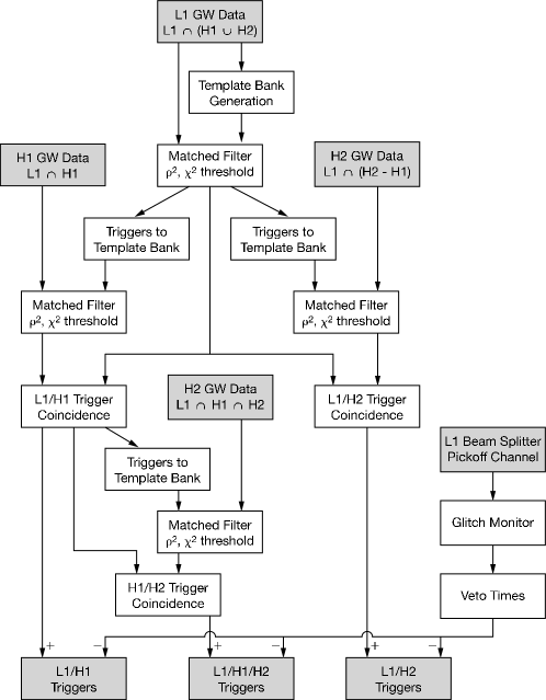
Figure 1: The triggered search pipeline. $\mathrm{L1}\cap(\mathrm{H1}\cup\mathrm{H2})$ indicates times when the L1 interferometer was operating in coincidence with one or both of the Hanford interferometers. $\mathrm{L1}\cap\mathrm{H1}$ indicates times when the L1 interferometer was operating in coincidence with the H1 interferometer. $\mathrm{L1}\cap(\mathrm{H2}-\mathrm{H1})$ indicates times when the L1 interferometer was operating in coincidence with only the H2 interferometer. The outputs of the search pipeline are triggers that belong to one of the two double coincident data sets or to the triple coincident data set.

This pipeline is equivalent to simply filtering the data from the three interferometers and looking for coincident triggers. The triggered search is more computationally efficient because H1 and H2 data is filtered only if it could possibly produce a coincident trigger, i.e., only for times when there are L1 triggers produced.

2.1 The datafind program

The datafind program [7] uses tables of science segments—lists of time when each interferometer was operating stably and producing “science mode” data—to identify data chunks to be used in the analysis. The chunks are composed of 15 overlapping analysis segments of 256 s which are used for power spectral density (PSD) estimation and for matched filtering with the findchirp algorithm. For the S2 inspiral analysis chunks of 2048 s were used and are chosen so that they overlap by 128 s to allow continuous filtering across the boundary between chunks (though the last chunk in a science segment overlaps by a larger amount so that it can remain 2048 s long). Figure 2 shows how analysis chunks are constructed from science segments in S2.

Figure 2: The algorithm used to divide science segments into data analysis segments. Science segments are divided into $2048$ s chunks overlapped by $128$ s. (Science segments shorter than $2048$ s are ignored.) An additional chunk with a larger overlap is added to cover any remaining data at the end of a science segment. Each chunk is divided into $15$ analysis segments of length $256$ s for filtering. The first and last $64$ s of each analysis segment is ignored, so the segments overlap by $128$ s. Areas shaded black are filtered for triggers by the search pipeline. The gray area in the last chunk of the science segment is not searched for triggers as this time is covered by the preceding chunk, however this data is used in the PSD estimate for the final chunk.

2.2 The tmpltbank program

The tmpltbank program [8] is responsible for producing a bank of waveform templates to be used as matched filters by the inspiral program. In the triggered search pipeline the L1 data is filtered first and since the coincidence stage requires triggers to be observed in the same template (see below), it is sufficient to generate a template bank suitable for the L1 data. To construct a template bank tmpltbank needs an estimate of the average strain noise PSD of the instrument. This is computed for each data analysis chunk (as provided by datafind) using the same method as the inspiral code. The specific templates that produce inspiral triggers in the inspiral program will then be used as the bank for subsequent analyses of H1 and/or H2 data.

The S2 inspiral and MACHO searches looked for signals from binary systems where the component masses were in the range $1\,M_{\odot}\leq m_{1},m_{2}\leq 3M_{\odot}$ (the binary neutron stars) and the range $0.2\,M_{\odot}\leq m_{1},m_{2}\leq 1M_{\odot}$ (the binary black hole MACHOs). Since each mass pair $m_{1},m_{2}$ in the space produces a different waveform, we construct a template bank—a discrete subset of the continuous family of waveforms that belong to the parameter space. The placement of the templates in the bank is determined by the mismatch of the bank which is the maximum fractional loss of signal-to-noise ratio that can occur by filtering a true signal with component masses $m_{1},m_{2}$ with the “nearest” template waveform for a system with component masses $m_{1}^{\prime},m_{2}^{\prime}$. The construction of an appropriate template bank is discussed in Refs. [9, 10].

A typical choice for the maximum bank mismatch is 3%, which would correspond to a 10% loss of event rate for a population of sources with uniform spatial distribution. This 3% bank mismatch was adopted in the S2 binary neutron star search. Binary black hole MACHOs, if they exist, would exist in the Milky Way halo and would be easily detectable; it is not so important for the template bank to have such a small mismatch. By raising the mismatch, fewer templates are needed in the bank. This is an important computational-cost saving strategy for the binary black hole MACHO search as the template bank is very large for these very-low mass sources. For the S2 binary black hole MACHO search we adopted a mismatch of 5%.

2.3 The inspiral program

The inspiral program [8] is the driver for the findchirp algorithm, which is discussed in detail in [5]. This program acquires a chunk of data identified by datafind and the bank of templates produced by tmpltbank or trigbank. The inspiral program then (i) conditions the data by applying an 8th order Butterworth highpass filter with 10% attenuation at 100 Hz and resamples the data from 16384 Hz to 4096 Hz, (ii) acquires the current calibration information for the data, (iii) computes an average power spectrum from the 15 analysis segments, and (iv) filters the analysis segments against the bank of filter templates and applies the $\chi^{2}$ test for waveform consistency. These operations (apart from the data conditioning) are described in detail in the paper discussing the findchirp algorithm. The inspiral program requires several threshold levels: the signal-to-noise threshold $\rho_{\ast}$, the chi-squared threshold $\chi^{2}_{\ast}$, the number of bins $p$ to use in the chi-squared veto, and the parameter $\delta$ used to account for the mismatch of a signal with a template when implementing the chi-squared veto. Several additional parameters used by the inspiral program include the duration (and therefore the number) of analysis segments, the highpass filter order and frequency, the low-frequency cutoff for the waveform templates and the inverse spectrum truncation duration ($\pm 16$ s).

The inspiral program produces a list of inspiral triggers that have crossed the signal-to-noise ratio threshold and have survived the chi-squared veto. These triggers must then be confronted with triggers from other detectors to look for coincidences.

2.4 The trigbank program

The trigbank program [8] converts a list of triggers coming from inspiral and constructs an appropriate template bank that is optimized to minimize the computational cost in a follow-up stage. Only those templates that were found in one detector need to be used as filters in the follow-up analysis, and only the data segments of the second detector where triggers were found in the data from the first detector needs to be analyzed. Thus, in the S2 triggered search pipeline, only the L1 dataset needs to be fully analyzed; only a small fraction of the H1 and H2 datasets needs to be analyzed in the follow-up, and then only a fraction of the template bank needs to be used. The template bank produced by trigbank is read by the inspiral program that is run on the second detector’s data.

2.5 The inca program

The inspiral coincidence analysis, inca [8], performs several tests for consistency between triggers produced by inspiral output from analyzing data from two detectors. Triggers are said to be coincident if they have consistent start times (taken to be $\pm 1$ ms for coincidence between triggers from H1 and H2 and taken to be $\pm 11$ ms for coincidence between Hanford and Livingston triggers, where 10 ms is the light travel time between the two sites and 1 ms is taken to be the timing accuracy of our matched filter). The triggers must also be in the same waveform template and the measured effective distance, $D_{\mathrm{H1}}$ and $D_{\mathrm{H2}}$ in H1 and H2 respectively, of the putative inspiral must agree in triggers from H1 and H2: $|D_{\mathrm{H1}}-D_{\mathrm{H2}}|/D_{\mathrm{H1}}<\kappa+\epsilon/\rho_{\mathrm{H2}}$ where $\kappa$ and $\epsilon$ are tunable parameters and $\rho_{\mathrm{H2}}$ is the signal-to-noise ratio observed in H2. Such an amplitude consistency is not applied in the coincidence requirements between Hanford and Livingston triggers because the difference in detector alignment at the sites, while small, is significant enough that a significant fraction of possible signals could appear with large amplitudes ratios. In addition, in comparing Hanford triggers, it is important to not discard H1 triggers that fail to be coincident with H2 triggers merely because H2 was not sensitive enough to detect that trigger. Therefore H1/H2 coincidence is performed as follows: (1) For each H1 trigger compute $(1-\kappa)D_{\mathrm{H1}}/(1+\epsilon/\hat{\rho}_{\mathrm{H2}})$ (the lower bound on the allowed range of effective distance) and $(1+\kappa)D_{\mathrm{H1}}/(1-\epsilon/\hat{\rho}_{\mathrm{H2}})$ (the upper bound of the range). Here $\hat{\rho}_{\mathrm{H2}}$ is the anticipated signal-to-noise ratio of a trigger in H2 given the observed trigger in H1. (2) Compute the maximum range of H2 for the trigger mass. (3) If the lower bound on the effective distance is further away than can be seen in H2, keep the trigger (do not require coincidence in H2). (4) If the range of H2 lies between the lower and upper bounds on the effective distance, keep the trigger in H1. If an H2 trigger is found within the interval, store it as well. (5) If the upper bound on the distance is less than the range of H2, check for coincidence. If there is no coincident trigger discard the H1 trigger.

3 Construction of the search pipeline

In this section we demonstrate how the S2 triggered search pipeline in Fig. 1 can be abstracted into a DAG to execute the analysis. We illustrate the construction of the DAG with the short list of science segments shown in Table 1. For simplicity, we only describe the construction of the DAG for zero time lag results. (An artificial delay in the trigger time can be introduced to produce false coincidences—i.e., coincidences that cannot arise from astrophysical signals—as a means to obtain information on the background event rate. We refer to this as non-zero time-lag results.) The DAG we construct filters more than the absolute minimum amount of data needed to cover all the double and triple coincident data, but since we were not computationally limited during S2, we chose simplicity over the maximum amount of optimization that we could have used.

Interferometer	Start Time (s)	End Time (s)	Duration (s)
L1	730000000	730010000	10000
L1	731001000	731006000	5000
L1	732000000	732003000	3000
H1	730004000	730013000	8000
H1	731000000	731002500	2500
H1	732000000	732003000	3000
H2	730002500	730008000	5500
H2	731004500	731007500	2500
H2	732000000	732003000	3000

Table 1: The fake science segments used to construct the DAG shown in figure 3. Start and end time is given in GPS time (seconds since 0h UTC 6 Jan 1980).

A DAG consists of nodes and edges. The nodes are the programs which are executed to perform the inspiral search pipeline. In the S2 triggered search pipeline, the possible nodes of the DAG are datafind, tmpltbank, inspiral, trigbank, and inca. The edges in the DAG define the relations between programs; these relations are determined in terms of parents and children, hence the directed nature of the DAG. A node in the DAG will not be executed until all of its parents have been successfully executed. There is no limit to the number of parents a node can have; it may be zero or many. In order for the DAG to be acyclic, no node can be a child of any node that depends on the execution of that node. By definition, there must be at least one node in the DAG with no parents. This node is executed first, followed by any other nodes who have no parents or whose parents have previously executed. The construction of a DAG allows us to ensure that inspiral triggers for two interferometers have been generated before looking for coincidence between the triggers, for example.

The S2 inspiral DAG is generated by a script which is an implementation of the logic of the S2 triggered search pipeline. The script reads in all science segments longer than $2048$ seconds and divides them into master analysis chunks. If there is data at the end of a science segment that is shorter than $2048$ seconds, the chunk is overlapped with the previous one, so that the chunk ends at the end of the science segment. An option is given to the inspiral code that ensures that no triggers are generated before this time and so no triggers are duplicated between chunks. Although the script generates all the master chunks for a given interferometer, not all of them will necessarily be filtered. Only those that overlap with double or triple coincident data are used for analysis. The master analysis chunks are constructed for L1, H1 and H2 separately by reading in the three science segment files. For example, the first L1 science segment in Table 1 is divided into the master chunks with GPS times 730000000–730002048, 730001920–730003968, 730003840–730005888, 730005760–730007808, 730007680–730009728, and 730007952–730010000 (with triggers starting at time 730009664).

The pipeline script next computes the disjoint regions of double and triple coincident data to be searched for triggers. 64 seconds is subtracted from the start and end of each science segment (since this data is not searched for triggers) and the script performs the correct intersection and unions of the science segments from each interferometer to generate the segments containing the times of science mode data to search. The L1/H1 double coincident segments are 730007936–730009936 and 731001064–731002436; the L1/H2 double coincident segments are 730002564–730004064 and 731004564–731005936; and the L1/H1/H2 triple coincident segments are 730004064–730007936 and 732000064–732002936. The GPS start and end times are thus given for each segment to be searched for triggers. The script uses this list of science data to decide which master analysis chunks need to be filtered. All L1 master chunks that overlap with H1 or H2 science data to be searched are filtered. An L1 template bank is generated for each master chunk and the L1 data is filtered using this bank. This produces two intermediate data products for each master chunk, which are stored as XML data. The intermediate data products are the template bank file, L1-TMPLTBANK-730000000-2048.xml, and the inspiral trigger file, L1-INSPIRAL-730000000-2048.xml. The GPS time in the filename corresponds to the start time of the master chunk filtered and the number before the .xml file extension is the length of the master chunk.

All H2 master chunks that overlap with the L1/H2 double coincident data to filter are then analyzed. For each H2 master chunk, a triggered template bank is generated from L1 triggers between the start and end time of the H2 master chunk. The triggered bank file generated is called H2-TRIGBANK_L1-730002500-2048.xml, where the GPS time corresponds to start time of the master H2 chunk to filter. All L1 master chunks that overlap with the H2 master chunk are used as input to the triggered bank generation to ensure that all necessary templates are filtered. The H2 master chunks are filtered using the triggered template bank for that master chunk to produce H2 triggers in files named H2-INSPIRAL_L1-730002500-2048.xml. The GPS start time in the file name is the start time of the H2 master chunk.

All H1 master chunks that overlap with either the L1/H1 double coincident data or the L1/H1/H2 triple coincident data are filtered. The bank and trigger generation is similar to the L1/H2 double coincident case. The triggered template bank is stored in a file names H1-TRIGBANK_L1-730004000-2048.xml and the triggers in a file named H1-INSPIRAL_L1-730004000-2048.xml where the GPS time in the file name is the GPS start time of the H1 master chunk. The H2 master chunks that overlap with the L1/H1/H2 triple coincident data are described below.

For each L1/H1 double coincident segment to search, an inca process is run to perform the coincidence test. The input to inca is all L1 and H1 master chunks that overlap the segment to search. The GPS start and stop times passed to inca are the start and stop times of the double coincident segment to search. The output is a file names H1-INCA_L1H1-730007936-2000.xml. The GPS start time in the file name is the start time of the double coincident segment. A similar procedure is followed for each L1/H2 double coincident segment to search. The output files from inca are named H2-INCA_L1H2-731004564-1372.xml, and so on.

For each L1/H1/H2 triple coincident segment, an inca process is run to create the L1/H1 coincident triggers for this segment. The input files are all L1 and H1 master chunks that overlap with the segment. The start and end times to inca are the start and end times of the segment. This creates a file named H1-INCA_L1H1T-730004064-3872.xml where the GPS start time and duration in the file name are those of the triple coincident segment to search. For coincidence between L1 and a Hanford interferometer, we only check for time and mass coincidence (the amplitude cut is disabled).

For each H2 master chunk that overlaps with triple coincident data, a triggered template bank is generated. The input file to the triggered bank generation is the inca file for the segment to filter that contains the master chunk. The start and end times of the triggered bank generation are the start and end times of the master chunk. This creates a file called H2-TRIGBANK_L1H1-730004420-2048.xml. The H2 master chunk is filtered through the inspiral code to produce a trigger file H2-INSPIRAL_L1H1-730004420-2048.xml.

For each triple coincident segment to filter, an inca is run between the H1 triggers from the L1H1T inca and the H2 triggers produced by the inspiral code. The input files are the H1 inca file H1-INCA_L1H1T-730004064-3872.xml and all H2 master chunk inspiral trigger files that overlap with this interval.

An H1/H2 coincidence step creates two files: H1-INCA_L1H1H2-730004064-3872.xml and H2-INCA_L1H1H2-730004064-3872.xml where the GPS start time and duration of the files are the start and duration of the triple coincident segment. The L1/H1 coincidence step is then executed again to discard any L1 triggers not coincident with the final list of H1 triggers. The input to the inca are the files L1-INCA_L1H1T-730004064-3872.xml and H1-INCA_L1H1H2-730004064-3872.xml. The output are the files L1-INCA_L1H1H2-730004064-3872.xml and H1-INCA_L1H1H2-730004064-3872.xml. The H1 input file is overwritten as it is identical to the H1 output file.

Finally, we obtain the data products of the search which contain the candidate trigger found by the S2 triggered search pipeline in these fake segments. For the fake segments described here, the final output files will be:

Double coincident L1/H1 data

L1-INCA_L1H1-730007936-2000.xml L1-INCA_L1H1-731001064-1372.xml
H1-INCA_L1H1-730007936-2000.xml H1-INCA_L1H1-731001064-1372.xml

Double coincident L1/H2 data

L1-INCA_L1H2-730002564-1500.xml L1-INCA_L1H2-731004564-1372.xml
H2-INCA_L1H2-730002564-1500.xml H2-INCA_L1H2-731004564-1372.xml

Triple coincident L1/H1/H2 data

L1-INCA_L1H1H2-730004064-3872.xml L1-INCA_L1H1H2-732000064-2872.xml
H1-INCA_L1H1H2-730004064-3872.xml H1-INCA_L1H1H2-732000064-2872.xml
H2-INCA_L1H1H2-730004064-3872.xml H2-INCA_L1H1H2-732000064-2872.xml

The DAG that results from the fake science segments given in Table 1 is shown graphically in Fig. 3. As the size of the input science segment files increase, so the number of nodes and vertices in the DAG increases, however the algorithm for generating the DAG remains the same. While the example DAG shown in Fig. 3 has only 76 nodes, the analysis of the full S2 data set required a DAG containing 6941 nodes (for the zero-lag analysis alone). The results of the execution of this DAG to analyze the S2 data will be reported in Refs. [3, 4].

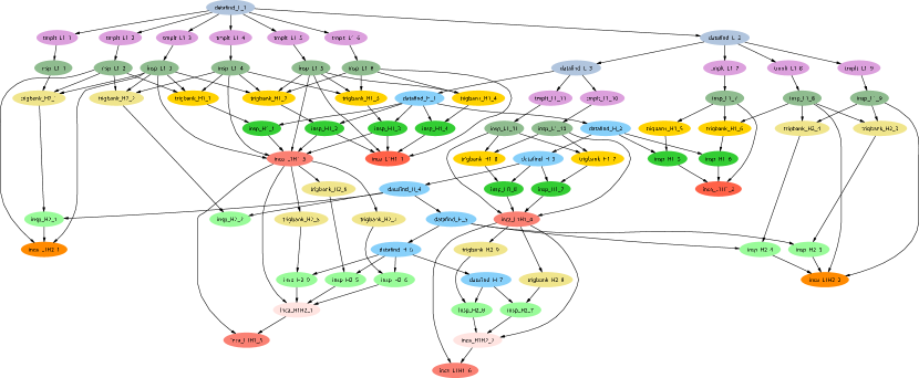
Figure 3: The DAG generated from the pipeline shown in figure 1 and the fake science segment list described in table 1. The figure shows the structure of the DAG with all job dependencies needed to execute the S2 triggered search pipeline. Note that it appears that there are several Hanford master chunks analyzed that do not need to be filtered for a zero time lag. These are added to the DAG to ensure that all the data necessary for a background estimation with a maximum time side of 500 seconds is analyzed.

References

References

- [1] B. Abbott et al. Phys. Rev. D 69, 122001 (2004).
- [2] E. Messaritaki (for the LIGO Scientific Collaboration) “Report on the first binary black hole inspiral search on LIGO data,” Submitted to Class. Quantum Grav.; B. Abbott et al. “LIGO search for gravitational waves from binary black hole mergers” (in preparation).
- [3] B. Abbott et al. “Search for gravitational waves from galactic and extra-galactic binary neutron stars” (in preparation).
- [4] B. Abbott et al. “Search for Gravitational Waves from Primordial Black Hole Binary Coalescences in the Galactic Halo” (in preparation).
- [5] D. A. Brown et al. “Searching for low-mass binary inspiral gravitational waveforms with the findchirp algorithm,” Submitted to Class. Quantum Grav.
- [6] Condor high throughput computing system, http://www.cs.wisc.edu/condor.
- [7] The datafind program is part of the Lightweight Data Replicator (LDR) http://www.lsc-group.phys.uwm.edu/LDR
- [8] The programs tmpltbank, inspiral, trigbank, and inca are in the LSC Algorithm Library Applications software package lalapps: http://www.lsc-group.phys.uwm.edu/daswg/projects/lalapps.html
- [9] B. J. Owen, Phys. Rev. D 53, 6749 (1996).
- [10] B. J. Owen and B. S. Sathyaprakash, Phys. Rev. D 60, 022002 (1999)