Accurate black hole evolutions by fourth-order numerical relativity

Abstract

We present techniques for successfully performing numerical relativity simulations of binary black holes with fourth-order accuracy. Our simulations are based on a new coding framework which currently supports higher order finite differencing for the BSSN formulation of Einstein’s equations, but which is designed to be readily applicable to a broad class of formulations. We apply our techniques to a standard set of numerical relativity test problems, demonstrating the fourth-order accuracy of the solutions. Finally we apply our approach to binary black hole head-on collisions, calculating the waveforms of gravitational radiation generated and demonstrating significant improvements in waveform accuracy over second-order methods with typically achievable numerical resolution.

I Introduction

Gravitational wave astronomy will soon provide astrophysicists with a new tool to observe and analyze some of the most energetic phenomena in our universe. Collisions of compact objects, such as neutron stars, stellar-mass black holes, and super-massive black holes, should produce characteristic gravitational wave signals that are observable to cosmological distances. In particular binary black hole systems are among the most promising sources of gravitational waves for both the current generation of ground-based detectors, such as LIGO Vogt (1992), and for the next generation of space-based detectors, such as LISA LIS ; Danzmann and Rudiger (2003). While early ground-based detectors will need to use templates from theoretically derived waveforms in order to extract the weak signal from the much larger noise, space-based detectors will require accurate models of the gravitational wave sources to extract the characteristic information (e.g., mass, spin) from the detected gravitational waves. Thus there is a critical need for accurate gravitational waveforms from realistic simulations of merging black holes.

Numerical studies of Einstein’s equations play an essential role in studying highly dynamic systems, such as binary black holes, that have little or no symmetry. These are not only computationally very demanding, requiring high-performance massive parallel computers, but also mathematically and numerically very challenging. Despite these difficulties a great deal of progress has been made in the last few years Alcubierre (2004), and it is now possible to follow binary black hole evolutions during the last moments of the merger phase Brandt et al. (2000); Alcubierre et al. (2001a, 2004a) and perhaps even through a complete orbit Brügmann et al. (2004). The calculation of the gravitational radiation emission from merging binary black holes has also been made possible through the use of the Lazarus approach, which bridges numerical relativity and perturbative techniques to extract approximate gravitational waveforms  Baker et al. (2001, 2002a, 2002b, 2004); Campanelli (2004). These calculations are in good agreement with recent numerical relativity evolutions  Alcubierre et al. (2004a).

At present, one of the most serious limiting factor in numerical relativity has been the inability to extract accurate and reliable results from stable three-dimensional numerical simulations of coalescing binary black hole spacetimes. Considerable resources have been dedicated to finding numerically stable formulations of the Einstein evolution equations Nakamura et al. (1987); Shibata and Nakamura (1995); Friedrich (1996); Frittelli and Reula (1996); Baumgarte and Shapiro (1999); Anderson and York (1999); Alcubierre et al. (2001a); Kidder et al. (2001); Sarbach and Tiglio (2002); Shinkai and Yoneda (2003); Lindblom and Scheel (2003); Bona and Palenzuela (2004). This effort has led to stable evolutions of single black hole spacetimes Alcubierre et al. (2001b); Yo et al. (2002); Alcubierre et al. (2003a); Sperhake et al. (2004). However, there is a growing realization that solving a well-posed formulation of the Einstein equations with second-order accurate finite differencing is not sufficient to produce accurate simulations of binary black hole spacetimes. Unfortunately, black hole simulations require large domains with high resolution near the horizons, and the unigrid second-order accurate codes developed in the past are not sufficient, given the foreseeable constraints on memory and CPU speed, to produce accurate waveforms from merging black holes Miller (2005). The Numerical Relativity community is currently pursuing several different approaches to produce accurate evolutions. Among them are the use of finite elements, spectral methods Pfeiffer et al. (2003); Kidder et al. (2000), adaptive mesh finite-difference codes Imbiriba et al. (2004); Fiske et al. (2005); Sperhake et al. (2005); Schnetter et al. (2004); Pretorius and Lehner (2004), and higher order finite-difference codes Calabrese et al. (2004). In addition, fourth-order accurate algorithms have recently been designed to evolve perturbations of nonrotating Lousto (2005) and rotating black holes Pazos-Avalos and Lousto (2004). Ideally, the next generation of finite-difference codes should combine higher order finite-differencing in combination with mesh refinement techniques. However, considerable progress toward highly accurate evolutions can be achieved using a unigrid higher-order finite-difference code along with a coordinate system, such as ‘Fisheye’ Baker et al. (2002a), that concentrates the gridpoints in the central region containing the black holes. In this paper we present a successful approach to performing fourth-order accurate numerical relativity simulations.

Our simulations are based on a new numerical relativity evolution code framework, LazEv, to solve the full non-linear Einstein’s equations in 3D. The LazEv framework is designed to be modular. The code consists of a ‘Method of Lines’ time integrator along with several Mathematica scripts Brügmann et al. that convert tensorial equations into finite-difference algorithms (of arbitrary order) in C. This modularity allows us to quickly implement new formulations and gauge choices as needed. We have currently implemented the ADM formulation as well as several ‘flavors’ of the BSSN formulation Nakamura et al. (1987); Shibata and Nakamura (1995); Baumgarte and Shapiro (1999). In Sec. II we describe the LazEv framework in detail. In Sec. III we enumerate many of the basic techniques utilized in numerical relativity simulations which we have implemented within LazEv, providing the foundation for detailed testing and application in black hole simulations.

In Sec. IV we test our fourth-order techniques on standard numerical relativity testbed problems Alcubierre et al. (2004b) demonstrating fourth-order accuracy. Finally, in Sec V we apply these methods to study head-on binary black hole collisions. Although head-on collisions have limited astrophysical relevance, there has been recent interest in using these spacetimes to develop and test numerical techniques for evolving more generic binary black hole spacetimes Alcubierre et al. (2004c); Fiske et al. (2005); Sperhake et al. (2005). In this paper we demonstrate that our fourth-order techniques can realize significant improvements in gravitational radiation waveform accuracies at typically achievable numerical resolutions.

II The LazEv Evolution Framework

The LazEv evolution framework is a foundation for rapid implementation of numerical relativity evolution system routines, supporting higher order finite differencing techniques with ‘method of lines’ (MoL) integration Gustafsson et al. (1995). Our numerical code uses the Cactus Computational Toolkit cactus_web for parallelization and IO. We have constructed the code so that it is compatible with the initial data and analysis thorns provided with Cactus. Specific evolution routines are produced using Mathematica scripts Brügmann et al. that convert tensorial equations into finite difference algorithms in C. These scripts provide several types of consistency checks that prevent many types of potential coding errors in setting up the tensorial equations. The Mathematica scripts support generic centered spatial finite differencing, with optional upwinded differencing (and other off-center differencing) provided by external macros. Currently we use second and fourth-order spatial finite differencing.

The LazEv framework applies the MoL technique for solving first-order-in-time, hyperbolic PDE’s, in which the PDE’s are converted into coupled ODE’s for all variables at every gridpoint. This is achieved by choosing a discrete numerical grid and finite difference stencils for the spatial derivatives (the finite different stencils couple the fields at neighboring gridpoints), and then integrating the time derivatives of the fields at all gridpoints. This time integration can be carried out by standard ODE integrators.

The LazEv MoL integrator provides a generic framework for integrating hyperbolic PDE’s using Runge-Kutta or ICN style time integrations. The integrator itself has no knowledge of the system that is being evolved. The MoL integrator provides internal timebins pre-ministep, ministep, dissipation, and post-ministep, which are called during each step of the Runge-Kutta or ICN integration (there are several ministeps in each full timestep). The evolution system is chosen by registering routines with MoL to be evaluated during each of these bins. For example, in the BSSN system (see Sec. III.1) we register routines to calculate the time derivative $\partial_{t}$ of all the BSSN variables in the ministep timebin, a routine to rescale the BSSN conformal metric $\tilde{\gamma}_{ij}$ to unit determinant in post-ministep, and a routine to subtract off the numerical trace of the BSSN trace-free, conformal extrinsic curvature $\tilde{A}_{ij}$ in post-ministep. In the ADM system, on the other hand, we register routines only in the ministep bin. Additional evolution systems may also register routines during these steps. For example, the gauge evolution systems, which are independent of the main evolution systems, also register routines in ministep and post-ministep.

Currently we have implemented ICN (second-order) and Runge-Kutta (second, third, and fourth-order). In some cases we use Kreiss-Oliger Kreiss and Oliger (1973) dissipation of the form

$$\partial_{t}F\to RHS+(-1)^{r/2}\epsilon\sum_{i}{h_{i}}^{r+1}{D_{i+}}^{r/2+1}{D_{i-}}^{r/2+1}\,F,$$ (1)

where $\partial_{t}F=RHS$ is one of the evolution equations, $h_{i}$ is the gridspacing in the $i$th direction, $D_{i+}$ and $D_{i-}$ are the forward and backwards differencing operators (in the $i$th direction), and $r$ is the order of the finite differencing used to evaluate $RHS$.

We use several different styles of finite difference stencils, depending on the order of accuracy desired and the type of derivative considered. Our standard choices for fourth-order accurate evolutions are:

$$\partial_{x}F_{i,j,k} = \frac{1}{12dx}(F_{i-2,j,k}-8F_{i-1,j,k}$$ (2)

$$+ 8F_{i+1,j,k}-F_{i+2,j,k}),$$

$$\partial_{xx}F_{i,j,k} = \frac{1}{12dx^{2}}(-F_{i+2,j,k}+16F_{i+1,j,k}$$ (3)

$$- 30F_{i,j,k}+16F_{i-1,j,k}-F_{i-2,j,k}),$$

$$\partial_{xy}F_{i,j,k} = \frac{1}{144dx\,dy}$$ (4)

$$[F_{i-2,j-2,k}-8F_{i-1,j-2,k}$$

$$+ 8F_{i+1,j-2,k}-F_{i+2,j-2,k}$$

$$- 8(F_{i-2,j-1,k}-8F_{i-1,j-1,k}$$

$$+ 8F_{i+1,j-1,k}-F_{i+2,j-1,k})$$

$$+ 8(F_{i-2,j+1,k}-8F_{i-1,j+1,k}$$

$$+ 8F_{i+1,j+1,k}-F_{i+2,j+1,k})$$

$$- (F_{i-2,j+2,k}-8F_{i-1,j+2,k}$$

$$+ 8F_{i+1,j+2,k}-F_{i+2,j+2,k})]$$

Note that the mixed $xy$ derivative is obtained by applying the x-derivative and y-derivatives sequentially (the order is irrelevant).

We do not use standard centered differencing for the advection terms (i.e. terms of form $\beta^{i}\partial_{i}F$). For these terms we use the following upwinded stencils:

$$\partial_{x}F_{i,j,k} = \frac{1}{12dx}$$ (5)

$$(-F_{i-3,j,k}+6F_{i-2,j,k}-18F_{i-1,j,k}$$

$$+ 10F_{i,j,k}+3F_{i+1,j,k})\mbox{\ \ \ for $\beta^{x}<0$}$$

$$\partial_{x}F_{i,j,k} = \frac{1}{12dx}$$ (6)

$$(F_{i+3,j,k}-6F_{i+2,j,k}+18F_{i+1,j,k}$$

$$- 10F_{i,j,k}-3F_{i-1,j,k})\mbox{\ \ \ for $\beta^{x}>0$}$$

In addition we use lower-order centered differencing on the planes adjacent to the boundaries. We have two choices for how the lower-order stencils are constructed. We can choose to use second-order centered differencing at all points on these planes and for all directions, or we can use second-order centered differencing only in the direction perpendicular to the boundary. When we use this latter choice we construct mixed second derivatives by applying the fourth-order accurate centered first derivative operator (in a direction tangent to the boundary) to the second-order centered derivative operator (perpendicular to the boundary).

Although we plan to implement excision boundary conditions soon, we currently use the puncture approach (see Ref. Alcubierre et al. (2004c) for a comparison of methods), along with singularity avoiding slicings, to evolve black hole space-times. When using punctures, we found that we needed to either use second-order stencils (but still fourth-order Runge-Kutta time integration) in regions inside the apparent horizons, or use a second-order upwinded stencil for the advection terms over the entire computational domain. The former method produces significantly better waveforms. See Sec. V.3 for further details.

III Formulation

Within our LazEv framework we have implemented support for several standard options in formulating numerical relativity modeling problems. Such a formulation includes selection of an Einstein evolution system and a choice of gauge for the evolving spacetime. In this section we discuss the formulation options presently available within our LazEv framework. Of these we have specific realizations which are appropriate for the fourth-order applications discussed in the subsequent sections.

III.1 Evolution Systems

Many alternative formulations of Einstein’s evolution equations have been considered so far (see Ref. Alcubierre et al. (2001c) and references therein). Within the most popular Cauchy or $3+1$ approach, one can currently choose among the first order symmetric hyperbolic formulations of the evolution equations which are mathematically very attractive Kidder et al. (2001); Sarbach and Tiglio (2002); Lindblom and Scheel (2003); Bona and Palenzuela (2004), and various flavors of spatially second-order hyperbolic formulations which are numerically more tractable Nagy et al. (2004); Gundlach and Martin-Garcia (2004). While the former have the advantage of possessing a well-posed continuum limit in the presence of maximally dissipative boundary conditions, it is not yet clear how one can handle dozens of free parameters Kidder et al. (2001); Sarbach and Tiglio (2002) and dynamical gauge choices for the lapse and shift. On the other hand, some second-order hyperbolic formulations have proven to be empirically much more robust than others Shibata and Nakamura (1995); Baumgarte and Shapiro (1999); Pretorius (2005); Kreiss and Ortiz ((2002). In this paper we will focus on the Baumgarte-Shapiro-Shibata-Nakamura (BSSN) Nakamura et al. (1987); Shibata and Nakamura (1995); Baumgarte and Shapiro (1999) system, a strongly hyperbolic system Sarbach et al. (2002); Beyer and Sarbach (2004) that has been shown to have some attractive stability properties Alcubierre et al. (2000); Sarbach et al. (2002); Beyer and Sarbach (2004).

The BSSN system is an extension of the standard ADM Arnowitt et al. (1962) system with better numerical properties than the original system. In the ADM system the Einstein Equations are split into six evolution equations for the metric (along with six auxiliary evolution equations for the extrinsic curvature)

$$\partial_{0}\gamma_{ij} = -2\alpha K_{ij},$$ (7)

$$\partial_{0}K_{ij} = -D_{i}D_{j}\alpha,$$ (8)

$$+\alpha(R_{ij}+KK_{ij}-2K_{ik}{K^{k}}{}_{j}),$$

and four constraints equations

$${\cal H} \equiv R+K^{2}-K_{ij}K^{ij}=0,$$ (9)

$${\cal M}^{i} \equiv D_{j}(K^{ij}-\gamma^{ij}K)=0.$$ (10)

Here $\partial_{0}$ is the operator $\partial_{t}-{\cal L}_{\beta}$, ${\cal L}_{\beta}$ is the Lie derivative with respect to the shift vector $\beta^{i}$, $D_{i}$ is the covariant derivative associated with the 3-metric $\gamma_{ij}$, $R_{ij}$ is the three-dimensional Ricci tensor, $R$ the Ricci scalar, and $K$ is the trace of $K_{ij}$.

The BSSN system of equations is obtained from the standard ADM equations by the following substitutions,

$$\gamma_{ij} \to e^{4\phi}\tilde{\gamma}_{ij},$$ (11)

$$K_{ij} \to e^{4\phi}\left(\tilde{A}_{ij}+\frac{1}{3}\tilde{\gamma}_{ij}K\right),$$ (12)

where $\tilde{\gamma}=\det\tilde{\gamma}_{ij}=1$ and $\tilde{A}^{i}_{\,i}=0$. Three additional variables

$$\tilde{\Gamma}^{i}=-\partial_{j}\tilde{\gamma}^{ij}$$ (13)

are also introduced. The BSSN variables ($\tilde{\gamma}_{ij}$, $\tilde{A}_{ij}$, $K$, $\phi$, and $\tilde{\Gamma}^{i}$) obey the following evolution equations Alcubierre et al. (2003b)

$$\partial_{0}\tilde{\gamma}_{ij} = -2\alpha\tilde{A}_{ij},$$ (14)

$$\partial_{0}\phi = -\frac{1}{6}\alpha K,$$ (15)

$$\partial_{0}\tilde{A}_{ij} = e^{-4\phi}\left(-D_{i}D_{j}\alpha+\alpha R_{ij}\right)^{TF}+$$ (16)

$$\alpha\left(K\tilde{A}_{ij}-2\tilde{A}_{ik}\tilde{A}^{k}_{\,j}\right),$$

$$\partial_{0}K = -D^{i}D_{i}\alpha+\alpha\left(\tilde{A}_{ij}\tilde{A}^{ij}+\frac{1}{3}K^{2}\right),$$ (17)

$$\partial_{t}\tilde{\Gamma}^{i} = \tilde{\gamma}^{jk}\partial_{j}\partial_{k}\beta^{i}+\frac{1}{3}\tilde{\gamma}^{ij}\partial_{j}\partial_{k}\beta^{k}+\beta^{j}\partial_{j}\tilde{\Gamma}^{i}-$$ (18)

$$\tilde{\Gamma}^{j}\partial_{j}\beta^{i}+\frac{2}{3}\tilde{\Gamma}^{i}\partial_{j}\beta^{j}-2\tilde{A}^{ij}\partial_{j}\alpha+$$

$$2\alpha\left(\tilde{\Gamma^{i}}_{jk}\tilde{A}^{jk}+6\tilde{A}^{ij}\partial_{j}\phi-\frac{2}{3}\tilde{\gamma}^{ij}\partial_{j}K\right),\hskip 28.45274pt$$

where $TF$ indicates that only the trace-free part of the tensor is used and $R_{ij}=\tilde{R}_{ij}+{R^{\phi}}_{ij}$ is given by

$${R^{\phi}}_{ij} = -2\tilde{D}_{i}\tilde{D}_{j}\phi-2\tilde{\gamma}_{ij}\tilde{D}^{k}\tilde{D}_{k}\phi+4\tilde{D}_{i}\phi\tilde{D}_{j}\phi-$$ (19)

$$4\tilde{\gamma}_{ij}\tilde{D}^{k}\phi\tilde{D}_{k}\phi,$$

$$\tilde{R}_{ij} = -\frac{1}{2}\tilde{\gamma}^{lm}\partial_{l}\partial_{m}\tilde{\gamma}_{ij}+\tilde{\gamma}_{k(i}\partial_{j)}\tilde{\Gamma}^{k}+\tilde{\Gamma}^{k}\tilde{\Gamma}_{(ij)k}+$$ (20)

$$\tilde{\gamma}^{lm}\left(2\tilde{\Gamma^{k}}_{l(i}\tilde{\Gamma}_{j)km}+\tilde{\Gamma^{k}}_{im}\tilde{\Gamma}_{klj}\right),$$

and $\tilde{D}_{i}$ is the covariant derivative with respect to $\tilde{\gamma}_{ij}$. $\tilde{\Gamma}^{i}$ is replaced by $-\partial_{j}\tilde{\gamma}^{ij}$ in Eq’s (14) - (20) wherever it is not differentiated. Note that Eq. (18) gives the $\partial_{t}$ derivative of $\tilde{\Gamma}^{i}$ rather than the $\partial_{0}$ derivative. The Lie derivatives of the non-tensorial quantities ($\phi$, $\tilde{\gamma}_{ij}$, and $\tilde{A}_{ij}$) are given by

$${\cal L}_{\beta}\phi = \beta^{k}\partial_{k}\phi+\frac{1}{6}\partial_{k}\beta^{k},$$ (21)

$${\cal L}_{\beta}\tilde{\gamma}_{ij} = \beta^{k}\partial_{k}\tilde{\gamma}_{ij}+\tilde{\gamma}_{ik}\partial_{j}\beta^{k}+$$ (22)

$$\tilde{\gamma}_{jk}\partial_{i}\beta^{k}-\frac{2}{3}\tilde{\gamma}_{ij}\partial_{k}\beta^{k},$$

$${\cal L}_{\beta}\tilde{A}_{ij} = \beta^{k}\partial_{k}\tilde{A}_{ij}+\tilde{A}_{ik}\partial_{j}\beta^{k}+$$ (23)

$$\tilde{A}_{jk}\partial_{i}\beta^{k}-\frac{2}{3}\tilde{A}_{ij}\partial_{k}\beta^{k}.$$

In addition to the evolution equations, the BSSN variables must also obey the following seven differential constraint equations

$${\cal H} = R-\tilde{A}_{ij}\tilde{A}^{ij}+\frac{2}{3}K^{2}=0,$$ (24)

$$e^{4\phi}\,{\cal M}^{i} = \partial_{j}\tilde{A}^{ij}+\tilde{\Gamma^{i}}_{jk}\tilde{A}^{jk}+6\tilde{A}^{ij}\partial_{j}\phi-$$ (25)

$$\frac{2}{3}\tilde{\gamma}^{ij}\partial_{j}K=0,$$

$${\cal G}^{i} = \tilde{\Gamma}^{i}+\partial_{j}\tilde{\gamma}^{ij}=0,$$ (26)

and the following two algebraic constraint equations

$$\tilde{\gamma} = 1,$$ (27)

$$\tilde{A}^{i}_{\,i} = 0.$$ (28)

We monitor the differential constraints but do not enforce them. However, we enforce the algebraic constraints by rescaling the evolved $\tilde{\gamma}_{ij}$ and subtracting off the trace of the evolved $\tilde{A}_{ij}$ at every timestep.

We can evaluate $(R_{ij})^{TF}=R_{ij}-1/3\gamma_{ij}R$ in two ways. We could either calculate $R_{ij}$ and find its trace $R$ numerically and subtract off the numerical trace, or we can use the Hamiltonian constraint Eq. (24) to calculate $R$ and subtract that from $R_{ij}$. Our tests showed very little difference between the two approaches even when the Hamiltonian constraint violations were relatively large. Unless otherwise specified we use the latter method.

III.2 Gauge Choices

We have implemented three basic types of lapse conditions: (i) maximal slicing, (ii) “Bona-Massó” type lapses Bona et al. (1995); Alcubierre et al. (2001b); Balakrishna et al. (1996); Alcubierre et al. (2003b), (ii) and densitized lapses. The maximal slicing condition has the form

$$\Delta\alpha=\beta^{i}\partial_{i}K+\alpha K_{ij}K^{ij},$$ (29)

and is implemented using a modified version of the Cactus ‘Maximal’ thorn cactus_web in combination with a fourth-order accurate version of Bernd Brügmann’s ‘BAM_Elliptic’ Brandt and Brügmann (1997); cactus_web thorn. This fourth-order accurate version of ‘BAM_Elliptic’ was developed at UTB by Mark Hannam. The “K-driver” lapses have the form

$$\partial_{t}\alpha=-\alpha^{2}f(\alpha)A,$$ (30)

where

$$\partial_{t}A=\partial_{t}K-\xi A,$$ (31)

and $\xi$ is some specified function (usually zero). We have also implemented modifications to this general form by replacing $\partial_{t}\alpha$ with $\partial_{0}\alpha$, adding $D_{i}\beta^{i}$ to the right-hand-side of Eq. (30), and multiplying $A$ by factors of $\psi^{n}$ in Eq. (30), where $\psi$ is the conformal factor of the puncture data. Equation (30) includes harmonic slicing ($f(\alpha)=1$), 1+log slicing ($f(\alpha)=2/\alpha$), and ‘shock-avoiding’ slicing ($f(\alpha)=\frac{8}{3}(\alpha(3-\alpha))^{-1}$) Alcubierre (2003).

We have implemented ‘Gamma-driver’ shift conditions Alcubierre et al. (2003b) as well as static corotating shifts. The two versions of the ‘Gamma-driver’ shifts that we implemented are

$$\partial_{t}\beta^{i} = F\,B^{i}-\zeta\,\beta^{i},$$

$$\partial_{t}B^{i} = \partial_{t}\tilde{\Gamma}^{i}-\eta B^{i},$$ (32)

and

$$\partial_{t}\beta^{i} = B^{i}-\zeta\,\beta^{i},$$

$$\partial_{t}B^{i} = F\,\partial_{t}\tilde{\Gamma}^{i}-\eta B^{i},$$ (33)

where $\eta$ and $\zeta$ are some prescribed functions over space, and $F$ is a function of $\alpha$ and $\psi$. Unless otherwise specified, we take $\zeta=0$.

III.3 Boundaries

Thus far we have implemented fairly simple boundary conditions. For fourth-order upwinded stencils we alternatively use centered finite differencing or second-order upwinding at the second point from the boundary, and second-order centered differencing at the first point from the boundary. The boundary points are filled using radiative boundary conditions Alcubierre et al. (2003b). However, when the shift is zero, or sufficiently small, we evolve $\tilde{\gamma}_{ij}$ on the boundary using the zero-shift form of Eq. (14). We have observed that the boundary algorithm has very little effect on the convergence of the $\ell=2$ component of the waveforms in Sec. V.

These boundary conditions are not known to be well posed and do lead to incoming constraint violating modes. Our future work will involve imposing constraint-preserving boundary conditions Gundlach and Martin-Garcia (2004); Frittelli and Gómez (2004); Calabrese et al. (2002).

IV Apples With Apples Tests

We apply the LazEv framework to a standard set of numerical relativity tests known as ‘Apples with Apples’ tests Alcubierre et al. (2004b). These tests consists of evolving spacetimes with $R\times T^{3}$ topology with the advantage that there are no boundaries. The results from these testbeds indicate that LazEv is stable and fourth-order convergent with our choices of fourth-order stencils.

IV.1 Gauge wave test

For this test we evolve the metric

$$ds^{2}=-H\,dt^{2}+H\,dx^{2}+dy^{2}+dz^{2},$$ (34)

where

$$H=1+A\,\sin\left(\frac{2\pi(x-t)}{d}\right),$$

and $d$ is the wavelength. The ADM variables for this metric have the form

$$\gamma_{xx} = 1+A\,\sin\left(\frac{2\pi(x-t)}{d}\right),$$ (35)

$$\gamma_{yy} = \gamma_{zz}=1,$$ (36)

$$K_{xx} = \frac{A\pi}{d}\frac{\cos\left(\frac{2\pi(x-t)}{d}\right)}{\sqrt{1+A\,\sin\left(\frac{2\pi(x-t)}{d}\right)}},$$ (37)

$$\alpha = \sqrt{1+A\,\sin\left(\frac{2\pi(x-t)}{d}\right)},$$ (38)

where all remaining ADM variables (including $\beta^{i}$) are zero. Note that $\alpha$ obeys the harmonic slicing condition

$$\partial_{t}\alpha=-\alpha^{2}K.$$ (39)

In our simulations $\alpha$ is ‘live’ and we evolve it using the harmonic slicing condition. A two-dimensional test is obtained by the coordinate transformation

$$x\to\frac{1}{\sqrt{2}}(x+y),$$

$$y\to\frac{1}{\sqrt{2}}(y-x),$$

producing non-trivial $\gamma_{xx}$, $\gamma_{yy}$, $K_{xx}$, and $K_{yy}$.

In order to obtain stable runs we needed to include dissipation of the form given in Eq. (1), with dissipation coefficient $\epsilon=0.125$.

These one and two-dimensional problems were evolved using a three-dimensional grid with periodic boundary conditions in all directions. We chose a wavelength ($d$) of 1 and constructed the grid so that it contained $6+1/h$ points (6 points for ghost-zones) in the non-trivial directions and 9 points in the trivial directions (the stencil requires 3 ghost-zones), where $h$ is the gridsize and $1/h$ is an integer.

Figure 1: The $L_{2}$ norm of $\delta\gamma_{xx}=\gamma_{xx}-\gamma_{xx}^{analytic}$, rescaled by $\rho^{4}/16$, for the one-dimensional ‘Gauge Wave’ test with $A=0.01$. Note the near perfect overlap for 630 crossing times and that the larger $\rho$ runs are convergent longer. The runs are acceptably accurate when the (non-rescaled) norm of the error is smaller than $10^{-4}$ (i.e. $1\%$ of $A$).

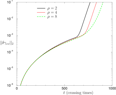
Our first test is a weak gauge wave with amplitude $A=0.01$ and resolutions $h=0.02/\rho$, where $\rho=$ $2$, $4$, $8$. Figure 1 shows the $L_{2}$ norm of the error in $\gamma_{xx}$ versus time (rescaled by a factor of $\rho^{4}/16$). Note that fourth-order convergence (as evident by the overlap of the rescaled curves) implies that the error for the $\rho=8$ case is 256 times smaller than the $\rho=2$ case. This relationship breaks down near $630$ crossing times, though the higher resolution runs remain in the convergence regime longer. Using the criterion that the numerical solution is sufficiently accurate if the norm of the error is smaller than $1\%$ of the amplitude $A$, we find that the fourth-order code produces accurate results to $t=308$, $t=720$, and $t=865$ for the $\rho=2$, $\rho=4$, and $\rho=8$ runs respectively.

Figure 2: The $L_{2}$ norm of ${\cal H}$, rescaled by $\rho^{4}/16$, for the one-dimensional ‘Gauge Wave’ test with $A=0.01$. Note the near perfect overlap for 800 crossing times and that the larger $\rho$ runs are convergent longer. The runs are acceptably accurate when the (non-rescaled) norm of the Hamiltonian constraint is smaller than $10^{-4}$ (i.e. $1\%$ of $A$)

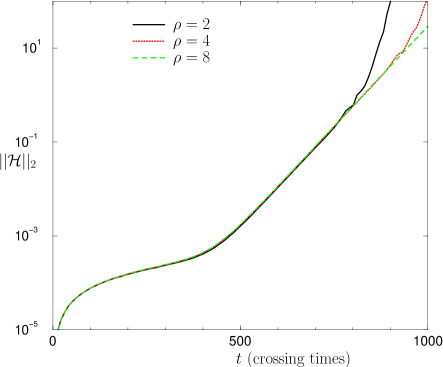
Figure 2 shows the $L_{2}$ norm of ${\cal H}$ (rescaled by a factor of $\rho^{4}/16$). Again, the higher resolution runs remain in the convergence regime longer. Using the criterion that the numerical solution is sufficiently accurate if the norm of the Hamiltonian constraint is smaller than $1\%$ of the amplitude $A$, we find that the fourth-order code produces accurate results to $t=130$, $t=495$, and $t=638$ for the $\rho=2$, $\rho=4$, and $\rho=8$ runs respectively. The Hamiltonian constrain violation is a stricter measure of the quality of the results than the error in $\gamma_{xx}$ because the Hamiltonian constraint involves second derivatives of the metric (which are harder to model).

Figure 3: The $L_{2}$ norm of ${\cal H}$, rescaled by $\rho^{4}/16$, for the one-dimensional ‘Gauge Wave’ test with $A=0.1$. Note the near perfect overlap for 80 crossing times and that the larger $\rho$ runs are convergent longer. The runs are acceptably accurate when the (non-rescaled) norm of the Hamiltonian constraint is smaller than $10^{-3}$ (i.e. $1\%$ of $A$).

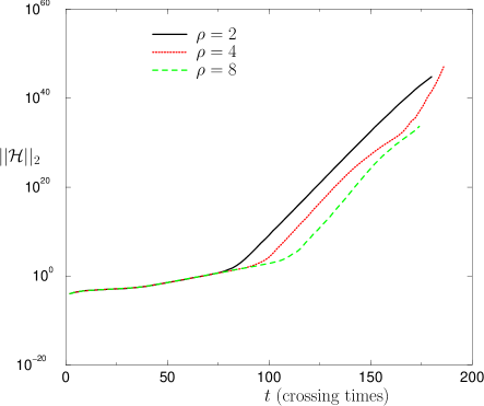
Our next test is a stronger gauge wave. Figure 3 shows the $L_{2}$ norm of ${\cal H}$ versus time (rescaled by a factor of $\rho^{4}/16$) for the gauge-wave test with amplitude $A=0.1$ and resolutions $h=0.02/\rho$, where $\rho=$ $2$, $4$, $8$. Note that in this higher amplitude case the runs remain convergent for 80 crossing times (approximately one-tenth as long as the $A=0.01$ runs). Using the criterion that the numerical solution is sufficiently accurate if the norm of the Hamiltonian constraint is smaller than $1\%$ of the amplitude $A$, we find that the fourth-order code produces accurate results to $t=19.5$, $t=46$, and $t=60$ for the $\rho=2$, $\rho=4$, and $\rho=8$ runs respectively. Hence these $A=0.1$ runs are accurate for roughly one-tenth the time that the $A=0.01$ are accurate.

Figure 4: The $L_{2}$ norm of ${\cal H}$, rescaled by $\rho^{4}/16$, for the two-dimensional ‘Gauge Wave’ test with $A=0.1$. Note the near perfect overlap for 55 crossing times and that the larger $\rho$ runs are convergent longer. The runs are acceptably accurate when the (non-rescaled) norm of the Hamiltonian constraint is smaller than $10^{-3}$ (i.e. $1\%$ of $A$).

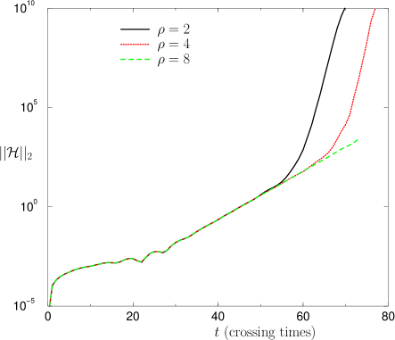
Though we have applied our fully three-dimensional code to the last two test problems, the dynamics in these cases are non-trivial only in one (numerical grid) direction. Our last gauge wave test is non-trivial in two grid directions. Figure 4 shows the $L_{2}$ norm of ${\cal H}$ versus time (rescaled by a factor of $\rho^{4}/16$) for the two-dimensional gauge-wave test with amplitude $A=0.1$ and resolutions $h=0.02/\rho$, where $\rho=$ $2$, $4$, $8$. These two-dimensional runs are less stable than the corresponding one-dimensional run, crashing before 100 crossing times. Convergence is, nonetheless, maintained for about 55 crossing times, longer for the higher resolution runs. Using the criterion that the numerical solution is sufficiently accurate if the norm of the Hamiltonian constraint is smaller than $1\%$ of the amplitude $A$, we find that the fourth-order code produces accurate results to $t=10$, $t=30$, and $t=40$ for the $\rho=2$, $\rho=4$, and $\rho=8$ runs respectively. Note that these two-dimensional $A=0.1$ runs are accurate roughly two-thirds as long as the corresponding one-dimensional $A=0.1$ runs.

IV.2 Gowdy wave test

In this section we present results for the ‘Polarized Gowdy Wave’ test. The ‘Polarized Gowdy Wave’ metric is given by

$$ds^{2}=t^{-1/2}e^{\lambda/2}(-dt^{2}+dz^{2})+t(e^{P}dx^{2}+e^{-P}dy^{2}),$$ (40)

where

$$P = J_{0}(2\pi t)\cos(2\pi z),$$ (41)

$$\lambda = -2\pi tJ_{0}(2\pi t)J_{1}(2\pi t)\cos^{2}(2\pi z)+$$ (42)

$$2\pi^{2}z^{2}\left[J_{0}^{2}(2\pi t)+J_{1}^{2}(2\pi t)\right]-$$

$$\frac{1}{2}((2\pi)^{2}[J_{0}^{2}(2\pi)+J_{1}^{2}(2\pi)]-$$

$$2\pi J_{0}(2\pi)J_{1}(2\pi)).$$

We use this metric to obtain initial data and evolve backwards in time using the harmonic slicing condition. The above metric only varies as a function of $z$ and $t$ but we can obtain a two-dimensional problem by introducing new coordinates $x=\tilde{x}$, $y=\tilde{y}$, $z=\tilde{z}+\tilde{y}$.

Here again we use a full three-dimensional grid to solve one and two-dimensional problems. We use periodic boundary conditions in all directions, and our grid consists of $1/h$ points (plus 6 for ghost-zones) in the non-trivial directions, and 9 points in the trivial directions. Additionally, we needed to add dissipation of the form given in Eq. (1), with dissipation coefficient $\epsilon=0.000625$, to stabilize the runs.

Figure 5: The $L_{2}$ norm of ${\cal H}$, rescaled by $\rho^{4}/16$, for the one-dimensional ‘Gowdy Wave’ test. Note the good agreement between the curves for 1000 crossing times and that the evolution is backwards in time

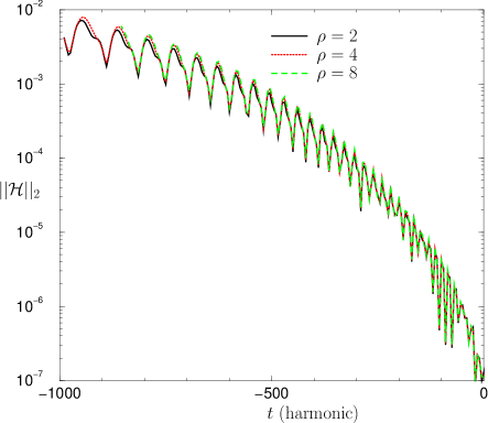
Figures 5 and 6 show the fourth-order convergence of the Hamiltonian constraint and the $\gamma_{zz}$ component of the metric of the one-dimensional Gowdy Wave test for 1000 crossing times. Note that these convergence plots imply that the errors in $\gamma_{zz}$ and ${\cal H}$ in the $\rho=8$ run are 256 times smaller than these errors in the $\rho=2$ run. Unlike the previous gauge-wave test, here the amplitude of the metric functions are damped. So our criterion for an acceptable value of the Hamiltonian constrain violation is time dependent. In this case we will use the criterion that the error norm, divided by the norm of $\gamma_{zz}$, must be smaller than $1\%$. At the end of the run the $L_{2}$ of $\gamma_{zz}$ (the function, not the error) is of order 1. Both the Hamiltonian constraint and the error in $\gamma_{zz}$ are smaller than this quality criterion for all resolutions.

Figure 6: The $L_{2}$ norm of the error in $\gamma_{zz}$, rescaled by the $L_{2}$ norm of $\gamma_{zz}$ and by $\rho^{4}/16$, for the one-dimensional ‘Gowdy Wave’ test. Note the good agreement between the curves for 1000 crossing times and that the relative error in $\gamma_{zz}$ is less than $2\cdot 10^{-4}$ at 1000 crossing times. The evolution is backwards in time.

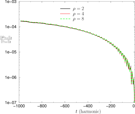
Figure 7 shows the fourth-order convergence of the Hamiltonian constraint for the two-dimensional Gowdy Wave test. The early time lack of convergence is due to roundoff effects, and, although the $\rho=2$ curve does not lie on the $\rho=4$ and $\rho=8$ curves, the overlap of the $\rho=4$ and $\rho=8$ curves confirm that the code is fourth-order convergent with sufficient resolution.

Figure 7: The $L_{2}$ norm of ${\cal H}$, rescaled by $\rho^{4}/16$, for the two-dimensional ‘Gowdy Wave’ test. The test was limited to 50 crossing times due to limited resources. The early time lack of convergence is due to low amplitude high frequency noise in the $\rho=8$ results. Although the two higher resolution curves do not lie on top of $\rho=2$ curve, the overlap of the two high resolution curves indicates that the Hamiltonian constraint is converging to fourth-order. Note that the evolution is backwards in time.

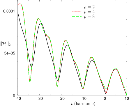
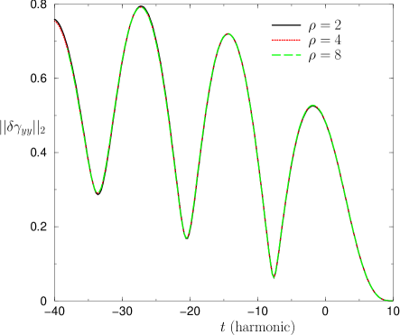
Figure 8 shows the fourth-order convergence of $\gamma_{yy}$ for the two-dimensional Gowdy Wave test. Unlike ${\cal H}$, $\gamma_{yy}$ clearly demonstrates fourth-order convergence at the low ($\rho=2$) resolution.

Figure 8: The $L_{2}$ norm of the error in $\gamma_{yy}$, rescaled by $\rho^{4}/16$, for the two-dimensional ‘Gowdy Wave’ test. The test was limited to 50 crossing times due to limited resources. The excellent overlap of all three curves indicates that the code is converging to fourth-order. Note that the evolution is backwards in time.

We conclude from the gauge wave and Gowdy wave results that our BSSN code is stable, accurate, and convergent.

V Head-on Binary Black-Hole Collisions

In this section we present results for head-on collisions of two equal-mass Misner-Wheeler-Brill-Lindquist (MWBL) black holes Brill and Lindquist (1963); Misner and Wheeler (1957). These results extend our previous tests of LazEv to more interesting nonlinear spacetimes containing binary black holes.

The MWBL data represent conformally flat slices of multiple black hole space-times with $n$ punctures. The data are parametrized by $n$ puncture masses $m_{i}$ and $n$ puncture positions ${\vec{r}_{i}}$ (in the conformal space). The ADM mass is given by the sum of $m_{i}$, and the ADM linear momentum and angular momentum are zero. The data have the form

$$\gamma_{ij} = \psi^{4}\delta_{ij},$$ (43)

$$K_{ij} = 0,$$ (44)

where

$$\psi=1+\sum_{i=1}^{n}\frac{m_{i}}{2r_{i}},$$ (45)

and $r_{i}=|{\vec{r}}-{\vec{r}_{i}}|$.

V.1 Setup

We used MWBL octant-symmetric data consisting of two equal mass black holes aligned along the z-axis, allowing us to evolve the data using the $\{x>0,y>0,z>0\}$ octant. In addition, we use a ‘Transition Fisheye’ transformation Baker et al. (2002a) to enlarge the physical domain without sacrificing resolution near the punctures. The ‘Transition Fisheye’ transformation is a smooth radial transformation from an inner resolution fixed by the Cactus gridspacing ($h$) to an outer resolution that is generally lower than the inner resolution. This transformation is parametrized by an outer ‘de-resolution parameter’ $a$ (the effective grid-spacing at the edge of the grid is $a\,h$), a transition width parameter ‘$s$’, and the center of the transition region ‘$r_{0}$’. The transformation has the form

$$r_{physical}=r(a+(1-a){\cal R}(r)),$$ (46)

where $r_{physical}$ is the physical radius corresponding to the coordinate radius $r$ and ${\cal R}(r)$ is given by

$${\cal R}(r)=\frac{s}{2r\tanh\frac{r_{0}}{s}}\ln\left(\frac{\cosh\frac{r+r_{0}}{s}}{\cosh\frac{r-r_{0}}{s}}\right).$$ (47)

For these runs we set the mass parameter of the two holes to $0.5M$, and the puncture positions to $(0,0,-1.1515M)$ and $(0,0,1.1515M)$. For most of the runs, the computational grid extended to $12.3M$, which corresponds to a physical size of $26M$. We also performed some short runs where the computational grid extended to $24.6M$, which corresponds to a physical size of $63M$. These latter runs were used to determine the effect of the boundaries on the waveforms, constraint violations, and horizon mass. The Fisheye parameters used in these runs were $a=3$, $s=1.2M$, $r_{0}=5.5M$. We performed runs at resolutions of $h=1.1515M/(9\rho)$ with gridsizes of $(96\rho)^{3}$ gridpoints along one octant, where $\rho=1,2,4$. The gridsizes were chosen so that the punctures lie halfway between gridpoints. For the runs with the boundary at $63M$ we used the same resolutions but chose gridsizes of $(192\rho)^{3}$ gridpoint along one octant, where $\rho=1,2$.

We evolved the data with the standard 1+log lapse, where the initial value of $A$ (see Eq. 31) is zero, and a modified 1+log lapse, where the initial value of $A$ is

$$A(t=0) = c\,\exp\left(-(\psi-1)^{-2}/\sigma\right).$$ (48)

We choose 1 for the initial value of the lapse. When using the modified lapse we set $c=0.5$, and $\sigma=0.8$. This modified lapse, unlike the original 1+log lapse, collapses at the puncture in the continuum limit. Analytically the standard 1+log lapse should retain its initial value at the puncture throughout the entire evolution. Since we start with a lapse of one, the lapse should not collapse at the puncture. However, the lapse will collapse near the puncture, and a lack of resolution drives the lapse to zero at the puncture as well. However, as the grid is refined this artificial collapse at the puncture is delayed, leading to short wavelength features and blow-ups near the puncture. The initial value of $A$ in Eq. (48) forces the lapse to collapse near the puncture in the continuum limit. Unfortunately this modification introduces its own problems as described below (see Fig. 21).

We used the second form of the ‘Gamma-Driver’ shift Eq. (III.2) to evolve the shift. The initial value of the shift and its time derivative were zero. We used both a constant $\eta$ ($\eta=2.8/M$) and a spatially varying $\eta$ equal to $2.8/M$ at infinity and $5.6/M$ at the punctures, as suggested by Diener Diener . The spatially varying $\eta$ was of the form Alcubierre et al. (2004c)

$$\eta=\eta_{p}-\frac{\eta_{p}-\eta_{\infty}}{(\psi-1)^{2}+1},$$ (49)

where $\eta_{p}$ and $\eta_{\infty}$ are parameters specifying $\eta$ at the puncture and infinity respectively, and $\psi$ is the puncture data conformal factor. The function $F$ in the ‘Gamma-Driver’ shift was set to $F=\frac{3}{4}\alpha/\psi^{4}$.

Pure fourth-order runs proved to be very unstable near the punctures both with and without upwinded stencils, and Kreiss-Oliger dissipation further destabilized these runs (near the punctures). We had success in stabilizing these runs with two techniques: (i) using second-order upwinding of advection terms over the entire grid, and (ii) a localized (within the apparent horizon) order reduction (LOR) to all second-order accurate spatial differentiation (including second-order upwinding of advection terms). This latter method provides significantly more accurate waveforms. When using the LOR method we found that lower-order accuracy is needed both at the punctures and at the origin. However, we only reduce the order of accuracy near the origin after a common apparent horizon forms (typically $5M$ after the common apparent horizon forms). We found that Kreiss-Oliger dissipation can be used to remove late time instabilities if the dissipation coefficient is set to zero in the LOR region. However, we did not use dissipation in the runs presented below.

We implement LOR in the following way. First we calculate the time derivatives of all variables using the standard fourth-order stencils in Eq’s (2) - (6). Then we overwrite all points within some given coordinate-ellipsoid with the time derivatives calculated using the standard second-order stencils (with second-order upwinded advection terms). The dissipation operator inside the LOR region can be either the same one chosen for the rest of the grid or a lower-order operator (in either case the dissipation coefficient inside the LOR region can be different from the dissipation coefficient used for the rest of the grid). Only the spatial finite differencing is changed; the time integrator is the same for all gridpoints. The size of the ellipsoid is chosen at runtime and up to eleven ellipsoids may be used. The user is free to choose when each ellipsoid is activated. For example, in the head-on binary black hole collision case, we specify a small ellipsoid for each of the individual apparent horizons and a larger ellipsoid for the common apparent horizon, where the larger ellipsoid is activated only after the common apparent horizons forms. The sizes of these ellipsoids can be determined by evolving with second-order accuracy over the entire grid and finding the sizes of the apparent horizons versus time.

For the head-on-collision runs the LOR regions consisted of spheres of radius $0.512M$ centered on the punctures activated at $t=2M$, as well as an ellipsoid with semi-axes $\{0.512M,0.512M,1.66M\}$ activated at $t=11.6M$ (the punctures were located on the z-axis). For comparison, the common apparent horizon has a minimum radius of $1.56M$ and a maximum radius of $1.88M$ at $t=11.4M$. The individual apparent horizons are approximately spherical with radii $0.61M$ at $t=1.98M$.

We used radiative boundary conditions for all variables except $\beta^{i}$ (which were evolved via $\partial_{t}\beta^{i}=B^{i}$ on the boundary). Table 1 gives the radiative boundary condition parameters for all variables. In Table 1 ‘$a$’ is the Fisheye de-resolution parameter. We enforce the algebraic constraints Eq’s (27),(28) prior to applying the boundary conditions. Hence, the boundary points do not satisfy these constraints exactly.

Table 1: Radiative Boundary Condition Parameters

Variables	Asymptote	speed
$\tilde{g}_{ii}$	$1$	$1/a$
$\tilde{g}_{ij}(i\neq j)$	$0$	$1/a$
$\tilde{A}_{ij}$	$0$	$1/a$
$\tilde{\Gamma}^{i}$	$0$	$1/a$
$\phi$	$(1/2)\ln(a)$	$\sqrt{2}/a$
$K$	0	$\sqrt{2}/a$
$\alpha$	0	$\sqrt{2}/a$
$B^{i}$	0	$1/a$
$A$	0	$1/a$

We updated the Zorro thorn of the Lazarus Toolkit Baker et al. (2002a) to compute the Weyl scalars to fourth-order accuracy and to make it compatible with octant, bitant, and quadrant symmetries in any direction as well as $\pi$ rotation symmetry about the z-axis. In addition we added a spherical harmonic decomposition routine to generate the $\ell=2$ and $\ell=4$ modes shown below.

V.2 Second-Order Accurate Results

We first confirmed that our code can reproduce the second-order accurate waveforms published in Alcubierre et al. (2003b). For these runs we used standard 1+log lapse (i.e. $A(0)=0$) and Gamma-Driver shift with $\eta=2.8$. We ran with gridsizes of $(96\rho)^{3}$ gridpoints and grid resolutions of $h=1.1515/(9\rho)$ for $\rho=1,2,4$. We calculated $\psi_{4}$ as well as its $(\ell=2,m=0)$ and $(\ell=4,m=0)$ components using Zorro Baker et al. (2002a). Note that the $(\ell=2,m=0)$ and $(\ell=4,m=0)$ modes of $\psi_{4}$ are purely real for this test.

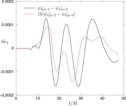
Figure 9 shows the $(\ell=2,m=0)$ mode of $\psi_{4}$ at $r=5M$ for these three resolutions along with the Richardson extrapolation of these data. In addition Fig. 9 shows the differences $4(\psi_{4}|_{\rho=2}-\psi_{4}|_{\rho=4})$ and $\psi_{4}|_{\rho=1}-\psi_{4}|_{\rho=2}$. These two difference curves overlap reasonably well indicating that the waveforms are second-order accurate. However, the phase drift between the two curves makes an evaluation of the exact order of convergence difficult. Figure 10 shows the convergence rate for this mode given by

$$\nu_{conv}=\log_{2}\frac{\psi_{4}|_{\rho=1}-\psi_{4}|_{\rho=2}}{\psi_{4}|_{\rho=2}-\psi_{4}|_{\rho=4}}.$$

The measured convergence rate oscillates wildly but averages to about 2.

Strictly speaking $r=5M$ is not in the radiation zone so $\psi_{4}$ given above does not represent the asymptotic waveform. However, the code’s performance in calculating the $(\ell=2,m=0)$ mode of $\psi_{4}$ at $r=5M$ is indicative of its performance in calculating this mode at large $r$. Additionally, boundary errors contaminate the $\ell=4$ modes at large $r$ (see Sec. V.3). Thus by extracting at $r=5M$ we can maximize the amount of non-trivial, physically correct quasinormal oscillations in the waveforms.

Figure 9: The top plot shows the $(\ell=2,m=0)$ mode of $\psi_{4}$ at $r=5M$ for the second-order evolution of the MWBL data for gridsizes $h=1.1515/(9\rho)$, as well as the Richardson extrapolated value. The bottom plot shows the differences $(\psi_{4}|_{\rho=1}-\psi_{4}|_{\rho=2})$ and $4(\psi_{4}|_{\rho=2}-\psi_{4}|_{\rho=4})$ between these waveforms for this mode. Note that the latter difference has been rescaled by a factor of four. Second-order convergence is demonstrated by the reasonable overlap between these two differences.

Figure 10: Convergence rate of the $(\ell=2,m=0)$ mode of $\psi_{4}$ at $r=5M$ for a purely second-order evolution of MWBL head-on collision data.

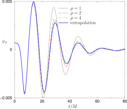
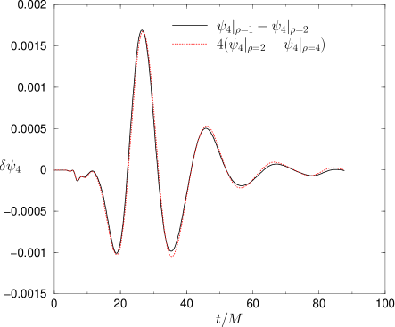
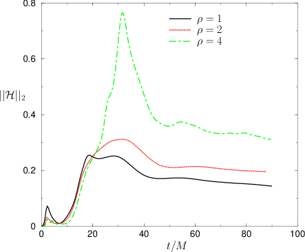
Figure 11 shows the $L_{2}$ norm of the Hamiltonian constraint for these three runs. Note that the constraints have not been rescaled. From the figure we can see that the constraints tend to get bigger as the resolution is increased. The source of these constraint violations is located between the puncture and origin. High frequency features develop there, leading to strong constraint violations. However, as seen in Fig. 12 these large constraint violations do not leak out of the apparent horizon. Thus, although there are significant problems inside the horizon, the region outside the horizon remains uncontaminated.

Our calculations of the gravitational waveforms from the Newman-Penrose scalar $\psi_{4}$, which contains higher-order spatial derivatives of the metric, do not reveal any additional degree of noise and distortion with respect the waveforms obtained from the Zerilli-Moncrief formalism Alcubierre et al. (2004c); Sperhake et al. (2005).

Figure 11: The $L_{2}$ norm of the Hamiltonian constraint violation versus time for the second-order accurate head-on collision runs. Note that the constraint violation increases with resolution.

Figure 12: Hamiltonian constraint violation (absolute value) versus $z$ along the z-axis at time $t=80M$ for the $\rho=4$ second-order head-on collision run. Note that the large constraint violation inside the apparent horizon ($r=2.8M$) has not leaked out into the exterior spacetime.

V.3 Fourth-Order Accurate Results

Purely fourth-order runs of puncture data proved to be unstable with more than one black hole. We found that we could stabilize the evolution by reducing the spatial discretization to second-order inside the apparent horizons, and we successfully ran the MWBL head-on collision data with fourth-order discretization, fourth-order Runge Kutta time integration, and second-order LOR regions inside the apparent horizons. For these runs we used the spatially varying $\eta$ form of the Gamma-driver shift given by Eq. (III.2) and Eq. (49). Figure 13 demonstrates the convergence of the $(\ell=2,m=0)$ component of $\psi_{4}$ at $r=5M$. Note that the system is not strictly fourth-order accurate. There appears to be an additional phase discrepancy between the two differences. However, the amplitude of the differences appears to be falling at a rate consistent with better than fourth-order accuracy. The $\rho=4$ run crashed at $47.5M$ due to an instability near the origin (see Fig. 19). This unstable mode was triggered by advection terms (the collapse of the lapse near the origin ensures that these are the only terms which can lead to a blowup). The fields which blew up most strongly were the $\tilde{\Gamma}^{i}$. This blow-up does not appear to be related to the quadratic blow-up in $\phi$ at the puncture discussed later. That term led to a blow up proportional to $e^{t^{2}}$ (in ${\cal H}$) near the puncture, which masked the unstable behavior near the origin. Both blow-ups can be modified by various choices in the gauge conditions and it is likely that a better choice of gauge will lead to longer fourth-order evolutions.

A fit of the $(\ell=2,m=0)$ mode of $\psi_{4}$ to the quasinormal form $f\sim e^{-at}\sin(\omega t)$ gave an exponential damping factor of $a=0.084/M$ and frequency of $\omega=0.373/M$. The exponential damping factor agrees to within 6% of the expected value of $0.0889625/M$, and the frequency agrees to within $0.2\%$ of the expected value of $0.373672/M$ Nollert and Schmidt (1992).

Figure 13: The top plot shows the $(\ell=2,m=0)$ mode of $\psi_{4}$ at $r=5M$, produced using fourth-order evolution with LOR, for 3 resolutions, along with the Richardson extrapolation curve of these data. The $\rho=2$ and $\rho=4$ curves are indistinguishable from the extrapolated curve. The bottom plot shows rescaled differences $\psi_{4}|_{\rho=1}-\psi_{4}|_{\rho=2}$ and $16(\psi_{4}|_{\rho=2}-\psi_{4}|_{\rho=4})$ (note the factor of 16). The convergence rate for the fourth-order runs using LOR inside the apparent horizons is not strictly fourth-order due to the phase discrepancy between the two curves, but average waveform differences between resolutions is consistent with fourth-order accuracy. Note that the amplitude of the dotted curve is less than the amplitude of the solid curve indicating better than fourth-order reduction in the amplitude of the errors.

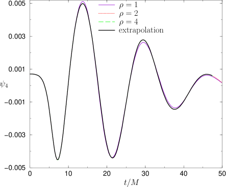
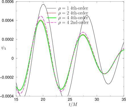
In Fig. 14 we show the Richardson extrapolated value of the $(\ell=2,m=0)$ mode of $\psi_{4}$, calculated using the second-order accurate results, along with the values obtained from second and fourth-order evolutions with LOR. Note that the medium resolution fourth-order run outperforms the high resolution second-order run. Figure 15 shows a magnified view of Fig. 14 (note that the legends in the two figures are different).

Figure 14: A comparison of the $(\ell=2,m=0)$ mode of $\psi_{4}$ at $r=5M$ for second and fourth-order evolutions with LOR. Note that the $\rho=1$ fourth-order waveform is better than the $\rho=2$ second-order waveform. Similarly the $\rho=2$ fourth-order waveform is better than the $\rho=4$ second-order waveforms. The Richardson extrapolated waveform (based on the second-order waveforms) is indistinguishable from the $\rho=2$ and $\rho=4$ fourth-order waveforms.

Figure 15: A comparison of the $(\ell=2,m=0)$ mode of $\psi_{4}$ at $r=5M$ for second and fourth-order evolutions with LOR. Note that the $\rho=2$ fourth-order waveform is better than the $\rho=4$ second-order waveforms. The second-order $\rho=4$ curve lies above the extrapolated curve while the fourth-order $\rho=1$ curve lies below.

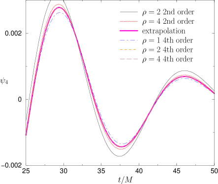
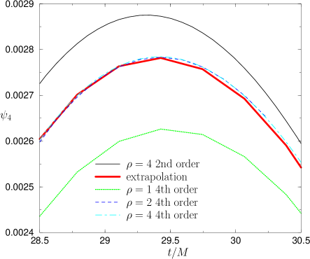
Figure 16 shows the convergence of the $(\ell=4,m=0)$ mode of $\psi_{4}$ at $r=5M$ calculated using fourth-order accuracy with LOR. The plot shows the differences $\psi_{4}|_{\rho=1}-\psi_{4}|_{\rho=2}$ and $16(\psi_{4}|_{\rho=2}-\psi_{4}|_{\rho=4})$, as well the mode itself for $\rho=4$. Note that the latter rescaled difference is smaller than the former. This indicates that the $(\ell=4,m=0)$ component of the waveform is converging faster than fourth-order. In addition, note that the error in the $\rho=1$ waveform is comparable to the amplitude of the waveform.

Figure 16: The $(\ell=4,m=0)$ mode of $\psi_{4}$ for $\rho=4$ as well as the differences between the $\rho=1$ and $\rho=2$ waveforms and the $\rho=2$ and $\rho=4$ waveforms (the latter rescaled by 16). The convergence rate of the $(\ell=4,m=0)$ mode of $\psi_{4}$ at $r=5M$ for the fourth-order runs with LOR is better than fourth-order. Note that the error in the $\rho=1$ waveform (as evident by the difference between the $\rho=1$ and $\rho=2$ waveforms) is approximately $50\%$ of the amplitude of the waveform at $20M$ and larger than the waveform beyond $30M$.

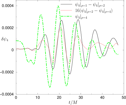
Figure 17 shows a magnified view of the $(\ell=4,m=0)$ mode of $\psi_{4}$ at $r=5M$ for the $\rho=1$, $\rho=2$, and $\rho=4$ fourth-order runs as well as the $\rho=4$ second-order run. Note that the $\rho=4$ second-order results are again inferior to the $\rho=2$ fourth-order (with LOR) results.

Figure 17: The $(\ell=4,m=0)$ mode of $\psi_{4}$ at $r=5M$ for fourth-order evolutions with LOR as well as second-order evolutions. Note that the $\rho=1$ fourth-order waveform has an order 100% error and that the $\rho=2$ fourth-order waveform has a substantially smaller error than the $\rho=4$ second-order waveform.

The $\ell=4$ modes, unlike the $\ell=2$ modes, contain significant contamination from the boundary at late times. For example, when extracting at $r=13M$ we find that the amplitude of the $(\ell=4,m=4)$ mode of $\psi_{4}$ (which is non-zero due to boundary errors) is approximately $50\%$ that of the $(\ell=4,m=0)$ mode at $t=45M$. This contamination is stronger when the extraction sphere is further out. However, the waveform extracted at $5M$ shows significantly less contamination. The reason for this is that the incoming error is delayed by about $8M$ while the outgoing mode is advanced by $8M$ (for a net gain of $16M$ in reliable data). In addition the outgoing mode, which has a $1/r$ falloff, is correspondingly larger at this smaller radius. This boundary contamination problem can be mitigated by pushing the outer boundary further out. This can be achieved within the existing LazEv framework using a stronger fisheye transformation or adding more gridpoints.

Although the waveforms from the fourth-order runs converge as expected the Hamiltonian constraint does not. High frequency features near the puncture and origin lead to large Hamiltonian constraint violation. At the points surrounding the puncture these high frequency features induce a quadratic blow-up in $\phi$ for the $\rho=4$ run. This quadratic behavior, which is confined to the nearest neighbor points to the puncture, leads to a blow-up of $e^{t^{2}}$ in the Hamiltonian constraint due to terms proportional to $e^{4\phi}$. This blow-up in ${\cal H}$ is entirely localized to the puncture and does not affect points outside. In the following figures we demonstrate that the large constraint violations inside the apparent horizon do not leak out and that the constraint violations outside the apparent horizon converge to zero when boundary effects are removed.

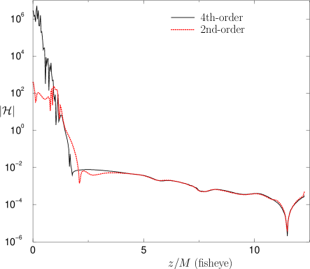
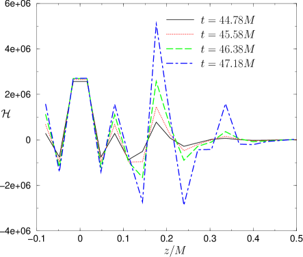
Figure 18 shows the Hamiltonian constraint along the z-axis (the points surrounding the puncture have been removed) at $t=47.2M$ for the second and fourth-order runs for $\rho=4$. The Hamiltonian constraint inside the horizon is as much as $10^{4}$ times larger for the fourth-order run. However, outside the horizon the constraint violations are very similar. Note that we do not expect the constraints to converge to zero in this case because our boundary conditions are not constraint preserving and boundary constraint violations have contaminated the solution at this time (the boundaries were at $26M$ in physical coordinates). The $\rho=4$ fourth-order run with LOR crashed due to an instability near the origin. Figure 19 shows the unstable mode in ${\cal H}$.

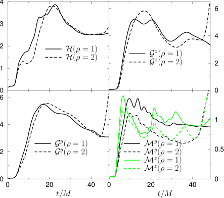
In Fig. 20 we show the $L_{2}$ norms of the Hamiltonian constraint ${\cal H}$, momentum constraint ${\cal M}^{i}$, and the BSSN constraints ${\cal G}^{i}$ (note that the $x$ and $y$ components of the both momentum and BSSN constraints are equal). We restricted these norms to the region outside $r_{physical}=3M$ (the horizon is at $r_{physical}\sim 2M$) and inside $r_{physical}=26M$, where $r_{physical}$ is the physical radius. The outer boundaries were located at $63M$ in physical coordinates. These runs required double the number of gridpoints (along each direction) as the standard runs for the same resolutions. The reasonable overlap of the $\rho=1$ and rescaled $\rho=2$ curves for $43M$ of evolution indicates that the $L_{2}$ norms are approximately fourth-order convergent (the convergence is lost near $t=40M$ due to constraint violating modes propagating in from the boundary). In addition, the amplitude of the constraint violations is $\sim 10^{-5}$, which is nine order of magnitude smaller than the maximum Hamiltonian violation inside the horizon. We conclude from this figure that the second-order errors introduced by the LOR differencing, as well as the extremely large Hamiltonian constraint violation inside the apparent horizon, do not propagate outside of the apparent horizon.

Figure 18: The absolute value of the Hamiltonian constraint along the z-axis at $t=47.2M$ for the second and fourth-order runs. The points near the puncture have been removed (the violation at the puncture was  $10^{117}$) from the fourth-order data. Note that the constraint violation is $10^{4}$ times bigger inside the horizon for the 4th order run, and that the extreme constraint violation does not leak out of the horizon (located at $z=2.8M$).

Figure 19: The unstable mode in ${\cal H}$ for the $\rho=4$ fourth-order runs.

Figure 20: The $L_{2}$ norm, restricted to the region $3M<r_{physical}<26M$, of all constraint violations. The boundaries were located at $63M$. All norms have been multiplied by $10^{5}$ and the $\rho=2$ norms have been rescaled by an additional factor of 16. In each panel the solid curves correspond to $\rho=1$ and the dashed curves to $\rho=2$. The reasonable overlap of the dashed and solid curves indicate that the constraint violations are converging to zero to fourth-order. The constraints no longer converge to zero after $t\sim 43M$ due to boundary effects.

The extreme Hamiltonian violation near the puncture can be removed using the modified 1+log lapse. However, this modification tends to destabilize the runs at late times. Figure 21 shows the $L_{2}$ norm of the Hamiltonian constraint violation for the $\rho=4$ fourth-order run with LOR. The modified lapse produces a constraint violation smaller than 1 for $25M$ but also causes the run to crash at $26.5M$. The standard 1+log lapse produces a “stable” evolution to $47.5M$ (see above) but has a constraint violation proportional to $e^{t^{2}}$ at the puncture. If short term evolutions, like the ones required for the Lazarus techniques, are required, then the modified 1+log is preferred.

Figure 21: The $L_{2}$ norm of the Hamiltonian constraint violation for the $\rho=4$ fourth-order evolution with LOR for the standard and modified 1+log lapses. Note the $e^{t^{2}}$ blow-up in the run using the standard 1+log lapse and that the run using the modified 1+log lapse crashes at $26.5M$.

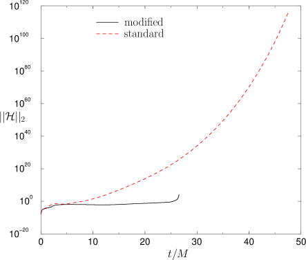
Figure 22 shows the horizon mass versus time, as calculated by the AHFinderDirect thorn Thornburg (2004), for the $\rho=2$ and $\rho=4$ runs with LOR. The plot also shows the horizon mass of a $\rho=2$ run with double the standard number of gridpoints in each direction and outer boundary at $63M$ in physical coordinates. The relatively sharp increase in the horizon mass at $t=32M$ is due to contamination from the boundary. When the boundary is moved out to $63M$ (from $26M$) this increase is delayed by roughly $\Delta t=37M$. Also note that the slope of the increase is reduced when the boundary is further out. The measured convergence rate of the horizon mass (based on runs with the boundary at $26M$) exceeded 3.8 for $30M$ of evolution.

Figure 22: The horizon mass versus time for the fourth-order runs with LOR. The thick solid line and the dotted line show the horizon mass versus time for the $\rho=2$ resolution with the physical boundary at $63M$ and $26M$ respectively. Note that the sharp increase in mass at later times is due to boundary effects. The dashed line shows the horizon mass for the $\rho=4$ run with the boundaries at $26M$. The error in the horizon mass at $t=63.5M$ is $2.6\%$ for the $\rho=2$ run with boundary at $26M$.

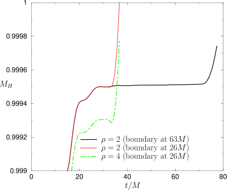
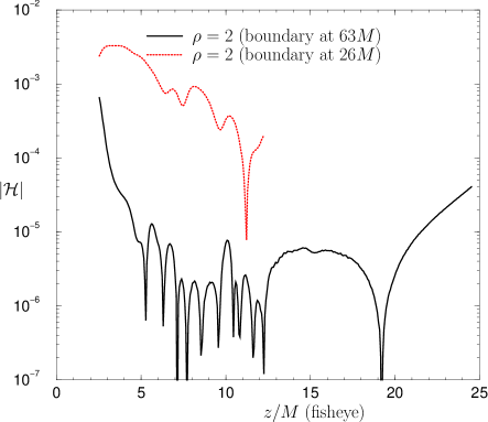
The horizon-mass versus time plot shows that the late time boundary contamination contains significant erroneous gravitational radiation. To determine when the calculated gravitational waveforms are good approximations to the true waveforms, we need to confirm that (i) the waveforms converge and do not change significantly when the resolution is further increased, (ii) the waveforms do not change significantly when the boundary effects are removed (which we achieved by causally disconnecting the boundaries from the observer), and (iii) the Hamiltonian constraint violation (inside the extraction region) is much smaller than the waveform amplitude. We have shown that the waveforms converge, and that the Hamiltonian constraint violation converges in the extraction region (see Fig. 20). Here we show the effects of the boundary on the Hamiltonian constraint and the waveforms. Figure 23 shows Hamiltonian constraint violation along the $z$ axis at time $t=40.8M$ for the standard $\rho=2$ run and a run with twice the standard number of gridpoints. The boundary in this latter case was at $63M$ (note that the $z$-axis plots the fisheye coordinate and that $z_{fisheye}=12.3M$ corresponds to the physical coordinate $z_{physical}=26M$ and $z_{fisheye}=24.6M$ corresponds to $z_{physical}=63M$). The figure shows the Hamiltonian constraint outside the apparent horizon. Note that at this time the boundary errors for the larger run have just reached $z_{fisheye}=12M$. The Hamiltonian constraint, in the range $z_{fisheye}=5M$ to $z_{fisheye}=12M$, is 100 times smaller for the run with the larger boundary. Even at $t=70M$, when the boundary errors have contaminated the entire grid, the Hamiltonian constraint is 20 times smaller for the larger run in this range.

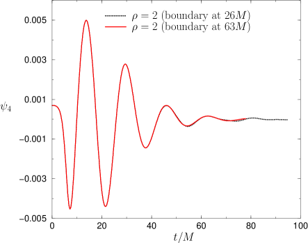
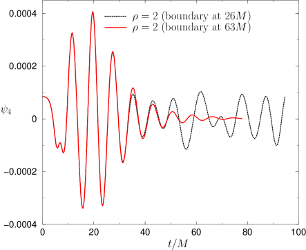
As seen in Fig. 24, the effect of reducing the boundary noise is not readily apparent in the $(\ell=2,m=0)$ mode of $\psi_{4}$. However, as seen in Fig. 25, the effect is readily observable in the $(\ell=4,m=0)$ mode. We conclude, based on these two figures, that the $(\ell=2,m=0)$ mode is represented accurately to $55M$ when the boundaries are located at $26M$, while the $(\ell=4,m=0)$ mode is represented accurately only to $33M$ for the same boundary location. The $(\ell=2,m=0)$ mode is more accurate because the boundary contamination contains relatively high frequencies which are filtered more effectively by the $(\ell=2,m=0)$ angular integration. Note that we placed the observer at $r=5M$ and that the waveforms become inaccurate sooner when the extraction sphere is placed at larger radii.

Figure 23: The Hamiltonian constraint along the $z$ axis at $t=40.8M$ for the fourth-order (with LOR) runs with gridspacing $h=1.1515/18$ (i.e. $\rho=2$). $z_{fisheye}=12.3M$ corresponds to $26M$ in physical coordinates and $z_{fisheye}=24.6M$ corresponds to $63M$ in physical coordinates. Boundary contamination for the larger run has just reached $z_{fisheye}=12M$. Note that in the range $5M<z_{fisheye}<12M$ the Hamiltonian constraint is 100 time smaller when the boundary is pushed out to $63M$.

Figure 24: The $(\ell=2,m=0)$ mode of $\psi_{4}$ (observer at $r=5M$) for the fourth-order (with LOR) $\rho=2$ run with the physical boundary at $26M$ (standard) and $63M$. The effect of the boundary is not significant until $t=55M$.

Figure 25: The $(\ell=4,m=0)$ mode of $\psi_{4}$ (observer at $r=5M$) for the fourth-order (with LOR) $\rho=2$ run with the physical boundary at $26M$ (standard) and $63M$. The effect of the boundary is significant at $t>33M$.

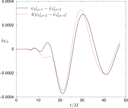
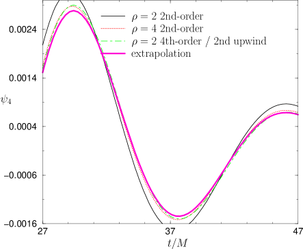
We conclude this section by showing the waveforms produced with fourth-order centered spatial finite differencing for all terms except the advection terms, for which we used second-order upwinded differencing. The waveforms produced by this method are inferior to those produced with LOR techniques but superior to those produced by the standard second-order technique. The time integration was carried out with the standard fourth-order Runge Kutta integrator. Figure 26 shows the differences $\psi_{4}|_{\rho=1}-\psi_{4}|_{\rho=2}$ and $\psi_{4}|_{\rho=2}-\psi_{4}|_{\rho=4}$ with the latter rescaled by 4 (to indicate second-order convergence) for the $(\ell=2,m=0)$ mode of $\psi_{4}$ at $r=5M$. The two curves do not overlap exactly due to phase drift. Despite the second-order accuracy of the algorithm, the waveforms produced with this technique are more accurate than those produced by the purely second-order spatial differencing. Figure 27 shows the $(\ell=2,m=0)$ mode of $\psi_{4}$ at $r=5M$ for the standard second-order evolution as well as the mixed fourth-order with second-order upwinding evolution. Note that the $\rho=2$ waveform from the latter technique is of a similar quality to the $\rho=4$ waveform from the purely second-order technique. The $\rho=4$ run crashed at $47.5M$ with the same mode that killed the $\rho=4$ LOR run. Both techniques crashed at the same time and in the same way because the instability near the origin is driven by advection terms, and both techniques use the same upwinded advection stencil near the origin. Figure 19 shows the unstable mode (along the z-axis) that crashes the $\rho=4$ fourth-order runs (with LOR and with second-order upwinding).

Figure 26: Convergence plot for the mixed fourth-ordered centered differencing with second-order upwinded differencing runs. Note that the difference $\psi_{4}|_{\rho=2}-\psi_{4}|_{\rho=4}$ has been multiplied by 4, indicating approximate second-order convergence.

Figure 27: A comparison of the $(\ell=2,m=0)$ mode of $\psi_{4}$ at $r=5M$ produced using the standard second-order evolution and a mixed fourth-order with second-order upwinding evolution. Note that the $\rho=2$ waveform from the mixed fourth-order/second-order upwinding is of similar quality to the $\rho=4$ second-order waveform. The extrapolated values used in this plot are based on the waveforms from the fourth-order runs with LOR.

We computed the energy radiated from the head-on collision by several different methods. We first estimated it by computing the difference between the final horizon mass and the total ADM mass, and obtained a radiated energy in the range $(7-8)\times 10^{-4}M$. We also used the Lazarus method to extract Cauchy data for the Teukolsky equation at relatively early evolution times $T\leq 20M$, and obtained $E_{radiated}=(8\pm 1)\times 10^{-4}M$. The direct integration of the $\ell=2$ and $\ell=4$ waveforms that we present here, extracted at numerical radii between $5M$ and $10M$, produce energy estimates of the order $\sim 6.6\times 10^{-4}M$.

VI Conclusion

We developed a new framework, LazEv, for evolving the Einstein equations using 3+1 decompositions. LazEv is capable of evolving with arbitrary-order finite difference stencils along with second, third, and fourth-order time integrators. The overall LazEv  design has a few novel features which will improve significantly upon previous setups which have been used in the Lazarus approach Baker et al. (2000, 2002a, 2001, 2002b, 2004). LazEv  is a flexible and modular evolution package, well-suited for rapid development and experimentation with well-posed hyperbolic systems of evolution equations, new ‘live’ gauge conditions, and sophisticated boundary conditions using arbitrary order finite differencing.

We implemented the BSSN formulation using this new framework and demonstrated that this new code passes the Apples with Apples testsuite and that the code reproduces the second-order accurate head-on binary black hole collisions waveforms published in Ref. Alcubierre et al. (2003b). We found that fourth-order accurate evolutions of the same data were not stable without some reduction of order and that the most accurate waveforms were obtained by evolving the data with second-order accurate stencils inside the apparent horizons and fourth-order stencils outside the horizon. In that case we found that the waveforms were fourth-order convergent and that the fourth-order accurate $192^{3}$ gridpoint runs outperformed the second-order-accurate $384^{3}$ gridpoint runs. This means that our fourth-order evolutions give better quality waveforms with over an order-of-magnitude smaller computational expense when compared to the second-order evolutions.

We also found that using a second-order upwinded stencil for the advection terms was sufficient to stabilize the runs. However, this introduces a second-order error in the waveform. Nevertheless, the waveforms produced by this latter method are superior to those produced by ordinary second-order accurate evolutions.

In this paper we demonstrated that the LazEv framework can be used to evolve binary black hole spacetimes. We plan to extend this work to include orbiting black holes starting from initial data based on the conformal thin-sandwich formulation Hannam as well as study recoil velocities from unequal mass head-on collisions Anninos and Brandt (1998). We also plan to extend the framework to include excision, fixed mesh refinement, constraint damping Marronetti (2005); Berger (2004), and constraint preserving boundary conditions.