Consistent discretizations: the Gowdy spacetimes

Abstract

We apply the consistent discretization scheme to general relativity particularized to the Gowdy space-times. This is the first time the framework has been applied in detail in a non-linear generally-covariant gravitational situation with local degrees of freedom. We show that the scheme can be correctly used to numerically evolve the space-times. We show that the resulting numerical schemes are convergent and preserve approximately the constraints as expected.

I Introduction

The “consistent discretization” approach DiGaPu has proven quite attractive to deal with conceptual issues in quantum gravity DiGaPubrasil . In this approach one approximates general relativity with a discrete theory that is constraint-free. As a consequence, it is free of the hard conceptual issues that plague quantum gravity. One can, for instance, solve the “problem of time” greece and one discovers that there is a fundamental decoherence njp ; cqg induced in quantum states that can yield the black hole information puzzle unobservable prl ; piombino .

A looming question in this approach is how well can the constraint-free discrete theory approximate general relativity? In this approach one starts with a Lagrangian, discretizes space-time and then works out discrete equations of motion that determine not just the usual variables of general relativity but the lapse and the shift as well. This has the attractive aspect of yielding a consistent set of discrete equations (they can all be solved simultaneously, unlike in usual discretizations where the constraints are not preserved upon evolution; it should be emphasized that preserving the constraints is becoming a central focus in state-of-the-art numerical relativity.) However, the resulting equations for determining the lapse and the shift are non-polynomial and of a rather high degree. Since these equations have no counterpart in the continuum theory, one does not have an underlying mathematical theory to analyze them as one has in the case of the other discrete equations. For instance, it is not obvious that the solutions of the equations will be real. Or that they do not oscillate wildly upon each step of evolution. We had probed these issues in some detail in some cosmological models cosmo . There the consistent discretization approach works well, approximating the continuum theory in a controlled fashion and covering all of the phase space. But in the cosmological case the equations also simplify significantly. Moreover, the diffeomorphism constraint does not play a role. In addition to this, it is known that discretizations of evolution equations can pose unique challenges. For instance, it is not clear that the resulting scheme produced by the consistent discretizations is hyperbolic in any given sense. With regular discretizations, the use of formulations that are not hyperbolic has led to problems. The type of discretizations that arise in the consistent discretization approach are also “forward in time centered in space”. This is due to the fact that the use of centered derivatives in time complicates the construction of the canonical formulation that is central to the use of consistent discretizations in quantum gravity. All this raised significant suspiciousness about how well these discretizations could approximate the continuum theory. An encouraging point was that at least for linearized gravity, the consistent discretizations yield a “mimetic” discretization mimetic that appears to be stable. But the linearized case has many peculiarities that do not carry over to the non-linear case (namely the mimetism). It is also true that at the classical level the “consistent discretization” approach may be considered as an extension of the idea of variational integrators to singular Lagrangians (systems with constraints treated in the Dirac fashion). Variational integrators have proven to have many desirable properties, at least for unconstrained systems (see variational for a recent review), but they have only been applied in a limited way to systems with constraints (only holonomic or at best constraints linear in the momenta mclc ) without treating them in the usual Dirac fashion.

It is clear that the viability of the approach has to be probed in situations with field-theoretical degrees of freedom. A situation of this type arises in the Gowdy cosmologies gowdy . These are spatially compact space-times with two space-like commuting Killing vector fields. This allows the introduction of coordinates where the metric depends only on time and an angular variable which we will call $\theta$. The consistent discretization approach applied to this model yields quite involved equations, as we will see. They cannot be solved analytically and have to be tackled numerically. Moreover, since we are dealing with non-linear coupled algebraic systems, the solution has to be constructed approximately, and the resulting systems are rather large. In addition to this, the presence of global constraints derived from the compact topology yields some of the systems unsolvable directly and this issue has to be addressed again by an approximate technique.

It should be made clear from the outset that we are not at all interested in being competitive in the well developed field of numerical simulations of Gowdy cosmologies (see Berger berger for a review). Usually numerical simulations of Gowdy take advantages of special gauges and other features that we will not take into account in our approach.

To simplify matters we will concentrate on the “single polarization” Gowdy case and we will further restrict to a particular subcase that can be seen as a “minisuperspace” by setting one of the variables and its conjugate momentum to zero. From the point of view of the evolution equations and the dynamics in terms of coordinate dependent quantities, the complexity of the equations is virtually similar to the full single-polarized case, one just is faced with a smaller number of equations. Moreover, if one were to write the full one polarization case and take suitably restricted initial data, the evolution is preserved exactly within the minisuperspace considered.

The organization of this article is as follows. In the next section we briefly review the formulation of Gowdy cosmologies mostly to fix notation. We then proceed to work out the consistent discretization. In section III we discuss the numerical scheme and present the numerical results.

II Gowdy cosmologies

II.1 Continuum formulation

Gowdy cosmologies are space-times with two space-like commuting Killing vector fields. We take the topology of the spatial slices to be a three-torus $T^{3}$. Following Misner misner , we parameterize the spatial metric by,

$$ds^{2}=e^{-\tau-(\lambda/2)}d\theta^{2}+e^{2\tau}\left(e^{\beta}d\sigma^{2}+e^{-\beta}d\delta^{2}\right)$$ (1)

where functions $\tau,\lambda,\beta$ depend on time $t$ and on one of the spatial variables which we call $\theta\in[0,2\pi]$. The other two spatial variables are $\sigma$ and $\delta$ and will play no role from now on. The Hilbert action particularized for these kinds of metrics reads,

$$S={1\over 2\pi}\int dt\int d\theta\left(p_{\lambda}\dot{\lambda}+p_{\tau}\dot{\tau}+p_{\beta}\dot{\beta}-{\bar{N}}_{\mu}{\bar{C}}^{\mu},\right)$$ (2)

where ${\bar{N}}_{\mu},\mu=0,1$ are related to the lapse and the single remaining component of the shift (Lagrange multipliers) by ${\bar{N}}=Ng^{-1/2}=N\exp(-3\tau/2+\lambda/4)$, ${\bar{N}}_{\theta}=N_{\theta}\exp\left(\tau+\lambda/2\right)$. Also ${\bar{C}}^{\mu}$ are related to the Hamiltonian and the single remaining component of the momentum constraint by the obvious rescalings,

$${\bar{C}}^{0} = {1\over 2}p_{\beta}^{2}+p_{\lambda}p_{\tau}+{1\over 2}e^{4\tau}\left(\beta^{\prime}\right)^{2}+e^{4\tau}\left(4\tau^{\prime\prime}+8\left(\tau^{\prime}\right)^{2}+\tau^{\prime}\lambda^{\prime}\right),$$ (3)

$${\bar{C}}^{\theta} = 4p_{\lambda}^{\prime}+p_{\tau}\tau^{\prime}+p_{\beta}\beta^{\prime}+p_{\lambda}\lambda^{\prime}.$$ (4)

We have also chosen the irrelevant spatial coordinates in such a way that $\int d\sigma\int d\delta=8$.

The theory can be consistently reduced by setting $\beta=p_{\beta}=0$. This corresponds to a one-parameter family of space-times. Since in our approach the coordinates are not fixed, the treatment is highly non-trivial, and the problem appears to be “infinite dimensional” (although one is strictly speaking dealing with a zero dimensional situation, as is the case in minisuperspaces). The exact solution of the evolution equations for this case can be written, in a given gauge choice (as shown by Misner). If one chooses lapse equal one, shift equal zero, $\tau^{\prime}=0$, $(p_{\lambda})^{\prime}=0$ one completely fixes gauge and the solution results $\tau=ct$, $p_{\lambda}=c$, $p_{\tau}=0$ and $\lambda=0$. We will see that in our approach we can choose initial data where the shift approximately vanishes upon evolution. This is good since it will allow us to compare scalars computed in the numerical solution with those of the exact solution. If the shift is non-vanishing then the situation complicates since one does not know at which points to compare the invariants (one is facing the classic “metric equivalence problem”, i.e., comparing metrics in two different coordinate systems to see if they are the same).

II.2 Consistent discretization

We now proceed to work out the consistent discretization of the theory. We assume that the time coordinate is related to a discrete variable $n$ by $t=n\Delta t$, $n=0\ldots N$. The spatial coordinate $\theta$ is also discretized $\theta=m\Delta\theta$ with $m=0\ldots M$. The action then becomes,

$$S = \sum_{n=0}L(n,n+1)$$ (16)

$$= \sum_{n=0}^{N}\sum_{m=0}^{M}\left\{\begin{array}[]{c}\\ \\ \end{array}p_{\lambda}(n,m)\left(\lambda(n+1,m)-\lambda(n,m)\right)+p_{\tau}(n,m)\left(\tau(n+1,m)-\tau(n,m)\right)\right.$$

$$-M(n,m)\left[p_{\lambda}(n,m)p_{\tau}(n,m)+e^{4\tau(n,m)}\left(4\tau(n,m+1)+4\tau(n,m-1)-8\tau(n,m)\begin{array}[]{c}\\ \\ \end{array}\right.\right.$$

$$\left.\left.+8\left(\tau(n,m+1)-\tau(n,m-1)\right)^{2}+\left(\tau(n,m+1)-\tau(n,m-1)\right)\left(\lambda(n,m+1)-\lambda(n,m-1)\right)\right)\right]$$

$$-N(n,m)\left[\begin{array}[]{c}\\ \\ \end{array}4p_{\lambda}(n,m+1)-4p_{\lambda}(n,m-1)\right.$$

$$\left.\left.+p_{\lambda}(n,m)\left(\lambda(n,m+1)-\lambda(n,m-1)\right)+p_{\tau}(n,m)\left(\tau(n,m+1)-\tau(n,m-1)\right)\begin{array}[]{c}\\ \\ \end{array}\right]\right\}$$

where we have rescaled the momenta $p(n,m)\equiv p(t,\theta)\Delta\theta$, and rescaled and relabeled the shift $N(n,m)\equiv\bar{N}_{\theta}(t,\theta)\Delta t/(\Delta\theta)$, and the lapse $M(n,m)\equiv\bar{N}(t,\theta)\Delta t/(\Delta\theta)$. The reader should keep in mind that in the rest of this paper when we refer to the “lapse” we are really referring at the lapse times the time interval in the discretization divided by the spatial interval. For example, we will therefore encounter statements like “making the lapse small” signifying that the discretization step, measured in an invariant fashion, is becoming smaller.

We now proceed to define the canonical variables from the action. The reader should not be confused by the use of variables named “p” in the action; in the consistent discretization scheme all variables are initially treated as configuration variables (i.e. one is working in a first order formulation of the theory, see jmp for a full discussion.) One defines canonical momenta at instant $n$ and at instant $n+1$. Let us consider for instance the variable $\lambda$. We define the canonical momenta at instant $n+1$ by,

$$P^{\lambda}(n+1,m)\equiv{\partial L\over\partial\lambda(n+1,m)}=p_{\lambda}(n,m)$$ (17)

and at instant $n+1$, using the Lagrange equations of motion one has,

$$P^{\lambda}(n,m)\equiv-{\partial L\over\partial\lambda(n,m)} = p_{\lambda}(n,m)+M(n,m-1)\left(\tau(n,m)-\tau(n,m-2)\right)-M(n,m+1)\left(\tau(n,m+2)-\tau(n,m)\right)$$ (18)

$$+N(n,m-1)p_{\lambda}(n,m-1)+N(n,m+1)p_{\lambda}(n,m+1).$$

One can combine these equations to eliminate the variable $p_{\lambda}(n,m)$ from the model and yield an evolution equation in terms of variables that are genuinely canonically conjugate,

$$P^{\lambda}(n+1,m) = P^{\lambda}(n,m)-M(n,m)e^{4\tau(n,m)}\left(\tau(n,m)-\tau(n,m+1)\right)-M(n,m-1)e^{4\tau(n,m-1)}\left(\tau(n,m)-\tau(n,m-1)\right)$$ (19)

$$+N(n,m)P^{\lambda}(n+1,m)-N(n,m-1)P^{\lambda}(n+1,m-1).$$

A similar procedure yields an (implicit) evolution equation for $P^{\tau}$,

$$P^{\tau}(n+1,m) = P^{\tau}(n,m)$$ (20)

$$-M(n,m)\left(4e^{4\tau(n,m)}\left(4\tau(n,m+1)+4\tau(n,m-1)-8\tau(n,m)+8\left(\tau(n,m+1)-\tau(n,m)\right)^{2}\right.\right.$$

$$+\left.\left.\left(\tau(n,m+1)-\tau(n,m)\right)\left(\lambda(n,m+1)-\lambda(n,m)\right)\frac{}{}\right)\right.$$

$$\left.+4e^{4\tau(n,m)}\left(-8-16\tau(n,m+1)+16\tau(n,m)+\lambda(n,m)-\lambda(n,m+1)\right)\right)$$

$$+N(n,m)P^{\tau}(n+1,m)-N(n,m-1)P^{\tau}(n+1,m-1)-4M(n,m+1)e^{4\tau(n,m+1)}$$

$$-M(n,m-1)e^{4\tau(n,m-1)}\left(4+16\tau(n,m)-16\tau(n,m-1)+\lambda(n,m)-\lambda(n,m-1)\right),$$

and for $\lambda$,

$$\lambda(n+1,m)=\lambda(n,m)+M(n,m)P^{\tau}(n+1,m)+N(n,m)\left(-4+\lambda(n,m+1)-\lambda(n,m)\right)+4N(n,m-1)$$ (21)

and $\tau$,

$$\tau(n+1,m)=\tau(n,m)+M(n,m)P^{\lambda}(n+1,m)+N(n,m)\left(\tau(n,m+1)-\tau(n,m)\right).$$ (22)

A similar treatment for the Lagrange multipliers (defining their canonical momenta and combining the equations at $n$ and $n+1$) yields the “pseudoconstraints”,

$$4P^{\lambda}(n+1,m+1)-4P^{\lambda}(n+1,m)$$

$$+P^{\lambda}(n+1,m)\left(\lambda(n,m+1)-\lambda(n,m)\right)+P^{\tau}(n+1,m)\left(\tau(n,m+1)-\tau(n,m)\right)=0$$ (23)

$$P^{\lambda}(n+1,m)P^{\tau}(n+1,m)+e^{4\tau(n,m)}\left[4\tau(n,m+1)+4\tau(n,m-1)-8\tau(n,m)\right.$$

$$\left.+8\left(\tau(n,m+1)-\tau(n,m)\right)^{2}+\left(\tau(n,m+1)-\tau(n,m)\right)\left(\lambda(n,m+1)-\lambda(n,m)\right)\right]=0.$$ (24)

The terminology “pseudoconstraints” reflects the fact that these equations can be seen as discretizations of the constraint equations of the continuum theory. However, they are not constraints for the discrete theory in the usual sense of the word since they involve variables at different instants of time.

The set of equations (19-24) constitute six nonlinear coupled algebraic equations for the six unknowns, $\tau,\lambda,P^{\tau},P^{\lambda},N,M$, that is, they determine the canonical variables and the Lagrange multipliers. In fact, this is an oversimplified view of the situation, since the equations link variables at different spatial points $m$. In order to solve them, one has to take into account that all variables in the Gowdy problem are periodic, for instance in a lattice with $mm$ points, $\tau(0)=\tau(mm)$, etc. and then one is left with a system of $6\times mm$ equations with $6\times mm$ unknowns. So if one decides to use 10 spatial points these are 60 equations with 60 unknowns.

In fact, one does not need to tackle the system in an entirely coupled fashion, since the two evolution equations for $\lambda$ and $\tau$ are explicit. We will discuss the solution strategy in more detail in the next section.

A final remark is that Van Putten proposed a scheme which also can be characterized as determining the lapse and shift, but it differs significant from ours (in particular it is not motivated variationally). He also applied it to the Gowdy cosmologies vp .

III Numerical results

III.1 Choice of initial data

In order to evolve the equations we need to set initial data. The choice of initial data is somewhat delicate, since it will determine not only the solution but also the lapse and the shift. Although one can give arbitrary initial data, it would be desirable if the resulting lapse were of the same sign across the spatial manifold. If one does not make this choice, the scheme is able to evolve, but portions of the spacetime will be evolved forward in time and some portions it will evolve backward in time. There is nothing wrong with this, but it is not what is traditionally considered in numerical evolutions. We may also wish to choose a vanishing shift, although this is not important.

In order to ensure that the lapse and shift are approximately in line with what we desire, we proceed in the following way. We start with some initial data for the variables $\tau(0),\lambda(0),N(0),M(0)$. We use equations (23,24) to determine $P^{\tau}(1),P^{\lambda}(1)$ and then we use equations (19,20) to determine $P^{\tau}(0),P^{\lambda}(0)$. This completes the initial data set. That is, we have given us $\tau,\lambda$ and the lapse and the shift that we desire, and this determined the canonically conjugate momenta.

At this point the reader may be confused. Usually in numerical relativity one gives the metric and its canonical momenta at a given hypersurface, and they are chosen in such a way that they satisfy the constraints. To implement the consistent discretization evolution in this case one would consider the metric as evaluated at $0$ and the canonical momenta evaluated at $1$. One then chooses lapse and shift at $0$ and evolves. Presumably one would choose a small lapse in order to generate an evolution that is close to the continuum theory (recall that we refer here to the rescaled lapse). One could do things the other way around, choosing the metric at $1$ and the canonical momentum at $0$ and evolve backwards. The choice we made to of initial data is equivalent to finding a solution of the usual constraints at a given hypersurface with $\lambda,\tau$ given.

III.2 Evolution

We need to give a prescription that, given $\tau(n),\lambda(n),P^{\tau}(n),P^{\lambda}(n)$ determines the variables at instance $n+1$ and in the process determines the Lagrange multipliers. One could take the complete set of equations and solve them simultaneously. We did not proceed like this. Since this was the first exploration of the system we thought it would be more instructive and offer more control on the situation to solve the equations in sub-systems. We will see however, that in the end one pays a price for this.

The scheme we used to solve the system is as follows: using equations (23,24) we determine $P^{\lambda}(n+1),P^{\tau}(n+1)$. We then take these values together with $\lambda(n),\tau(n),P^{\tau}(n),P^{\lambda}(n)$ and use the equations (19,20) to determine the Lagrange multipliers $N(n),M(n)$. With these multipliers and the initial values, it is possible, using (21,22) to determine $\lambda(n+1),\tau(n+1)$, which would complete the evolution process from level $n$ to $n+1$.

Unfortunately, there is a problem with this procedure. When we try to use equations (19,20) to determine $M(n),N(n)$ one finds that the system is indeterminate. One can determine all the Lagrange multipliers except one, which we can choose to be $M1\equiv M(n,m=1)$. This has to do with a symmetry of the Gowdy problem. The action (2) only depends on derivatives of the variable $\lambda$, therefore it is invariant under the addition of a constant to that variable. Using Noether’s theorem one can find out that there is a conserved quantity, $\int P^{\lambda}(\theta)d\theta$. A similar result holds in the discrete action, the conserved quantity becomes $\sum_{m=0}^{M}P^{\lambda}(m)$. If one imposes that this quantity be conserved, this can be used to determine entirely the Lagrange multipliers. Another way of seeing this is to notice that one can cast the conservation law as a constraint on the initial data,

$$\sum_{m=0}^{M}P^{\lambda}(n+1,m)[\lambda(n,m),\tau(n,m)]=\sum_{m=0}^{M}P^{\lambda}(n,m)$$ (25)

that is, writing the $P^{\lambda}$ at $n+1$ as a function of the initial data and imposing the conservation one has a constraint on the initial data. Imposition of this constraint is enough to determine entirely the Lagrange multipliers.

This is a pathology of our choice of scheme of solution of the coupled system of equations, dealing with it by parts. If we had chosen to solve the entire non-linear system (19,22) such system would have been well defined and would have automatically preserved the conserved quantity upon evolution. This would have, however, forced us to deal with a significantly larger coupled non-linear system.

Numerically, the way we will implement the conservation is to choose arbitrarily the value of one component of the lapse. We then run the evolution scheme we outlined and we will check if $\sum_{m=0}^{M}P^{\lambda}$ has varied. If it has, we will go back and adjust the arbitrary component of the lapse until the conserved quantity is kept constant. We will do this via a Newton–Raphson technique. The flow diagram of the logic is shown in figure 1. For the solution of the various non-linear systems we discussed we use the routine TENSOLVE tensolve .

Figure 1: The logic of the evolution scheme.

III.3 Results for the dynamical variables

In figure 2 we show the variable $\lambda$ as a function of the spatial points and as a function of time, for a simulation with 8 and 40 spatial points. The time is measured by the variable $\tau$, which is a good measure since it is invariant under coordinate changes of the $t,\theta$ variables. Since we have chosen the shift to be close to zero, and it is preserved that way upon evolution as we shall see, the value of the angle $\theta$ can be taken to be an invariant. We see that the variable $\lambda$ exhibits the types of oscillations of increasing frequency that one encounters in the exact solution for the Gowdy spacetime.

Figure 2: The variable $\lambda$ as a function of space ($\theta$) and time, measured by the variable $\tau$. We show two resolutions, one with 8 and another with 40 spatial points. The latter represents what is practical to run on a workstation today. One sees that the two resolutions track each other well for a while, but things deteriorate as time increases (see for instance the third line of crosses from the right). The run with 8 spatial points just does not have enough resolution to track the features of the solution in question, as can be seen from the figure.

The evolutions with different spatial resolutions all have the same initial data for $\lambda(0),\tau(0),M(0),N(0)$. The explicit form of initial data chosen are,

$$\tau(0,i) = -0.5+0.01\sin(2\pi i/M),$$ (26)

$$\lambda(0,i) = 0.001\sin(2\pi i/M)+0.0025\sin(4\pi i/M),$$ (27)

$$M(0,i) = 0.0005,$$ (28)

$$N(0,i) = 10^{-7}\sin(2\pi i/M).$$ (29)

Following the initial data construction we outlined before, this produces differing values of $P^{\lambda}(0),P^{\tau}(0)$ depending on the number of points of the spatial grid. As shown in figure 3 there is convergence in the form of the resulting $P^{\lambda}(0),P^{\tau}(0)$ when one refines the spatial grid.

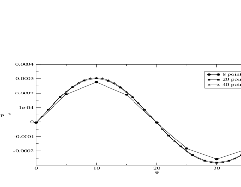
Figure 3: The variable $P^{\tau}$ in the initial data converges to a continuum solution of the pseudo-constraints, and would converge to a solution of the continuum usual constraints of GR if the choice of initial data for the lapse and shift were zero.

The $\lambda(0),\tau(0),P^{\lambda}(0),P^{\tau}(0)$ produced by the initial data solving procedure, in the limit in which one makes infinitely large the number of spatial points, is not a solution of the initial value constraints of the continuum theory. However one can approximate a solution of the constraints of the continuum theory arbitrarily by choosing the value of the initial (rescaled) lapse to be very small.

Figure 4 shows the value of the average of the shift across the grid as a function of time. We see that in all cases the shift is small, and is smaller for higher resolutions. This is desirable in order to compare with the exact solution which is in a gauge with zero shift.

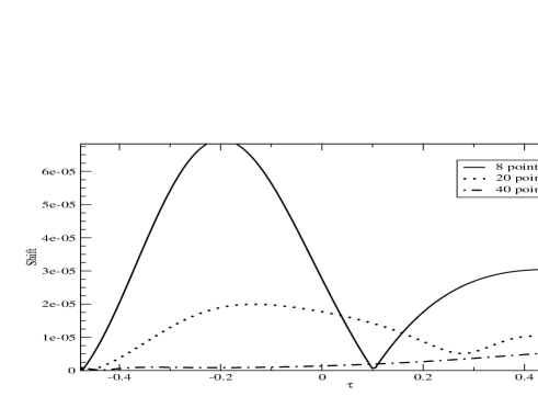
Figure 4: The L2 norm of the shift, which shows we are approximately in a gauge with zero shift.

Figure 5 shows the Riemann tensor for three resolutions. More precisely, it represents component $R_{3434}$ (where $3,4$ represent the ignorable coordinates) as a function of $\tau$ for $\theta=\pi$. The reason we chose this component is that it behaves as a scalar with respect to $t,\theta$ diffeomorphisms. Since we determine the lapse and the shift dynamically, for different resolutions we have different lapses and shifts and therefore different coordinates. As a consequence one cannot easily compare the other components of the Riemann tensor for different resolutions. One sees that the method converges, i.e. for smaller spatial separations the value of the Riemann tensor approximates well that of flat space-time.

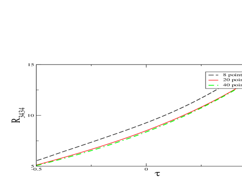
Figure 5: Convergence of the Riemann tensor for three different resolutions. Since we are working with an almost vanishing shift, the components of the Riemann tensor can be treated as observables and compared among different resolutions directly. With a non-vanishing dynamically determined shift this would not be possible. In such cases one can only compare observables of the theory.

We know the exact form of the Riemann tensor. In figure 6 we use it to evaluate the relative error in the evaluation. The exact form is $R_{3434}=c^{2}e^{-\tau}$ where $c$ is the only parameter present in the minisuperspace (recall $\tau=ct$). To avoid having to determine the constant we actually plot in figure 6 the following quantity,

$${{R_{3434}(\tau)\over R_{3434}(\tau(1))}-e^{-(\tau-\tau(1))}\over e^{-(\tau-\tau(1))}}$$ (30)

which yields the relative error.

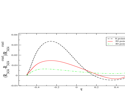
Figure 6: Relative error of the Riemann tensor compared to the exact solution.

In figure 7 we show the L2 norm of the square root of the sum of the squares of the constraints of the continuum theory evaluated in the discrete theory, for three resolutions. As expected, the magnitude of the constraints correlates well with the error in the evolution scheme.

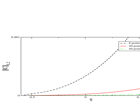
Figure 7: L2 norm of the constraints of the continuum theory evaluated in the discrete theory. As can be seen they are preserved well and in a convergent fashion. As argued in the text, the value of the constraints is a measure of the error of the evolutions in the discrete theory and this plot confirms it.

We are displaying the values of the constraints with any type of normalization. This may be misleading. As we see, although there is convergence there is also exponential growth. The growth can be adscribed to the general exponential growth of variables in Gowdy, particularly the factor $\exp(4\tau)$ that appears in the Hamiltonian constraint. To compensate for this in figure 8 we display the same data divided by the offending factor, and one cannot distinguish constraint growth.

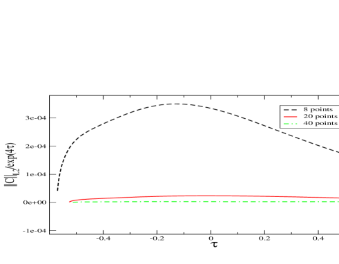
Figure 8: L2 norm of the constraints of the continuum theory evaluated in the discrete theory normalized by the factor $\exp(4\tau)$ that appears in the Hamiltonian constraint. One sees convergence with absence of growth in the normalized constraints. The reader may be puzzled as to why the curves do not start at the same point. The reason is that we are displaying the curves starting at the first iteration, not at the initial data. For very low resolutions the variables change quite a bit in the first iteration.

III.4 The flat sector

If one chooses initial data for the evolution equations (19,20,21,22) such that $P^{\lambda}=0$ and $\tau=0$, one can check that, in the continuum theory, one is producing flat space-time. We would like to check if the discrete theory is able to reproduce, at least in an approximate way, this behavior. This is usually known as the “gauge wave test” as is described, for instance in the “apples with apples” (www.appleswithapples.org) project, and it is known to be a somewhat significant hurdle for codes to pass (at least in full 3D).

In the discrete theory the pseudo-constraints (23,24) are identically satisfied and the lapse and shift are free. Let us start by considering a slicing with $M=1,N=0$. There are only two evolution equations left,

$$P^{\tau}(n+1,m) = P^{\tau}(n,m)+\lambda(n,m+1)-2\lambda(n,m)+\lambda(n,m-1)$$ (31)

$$\lambda(n+1,m) = P^{\tau}(n+1,m)+\lambda(n,m).$$ (32)

These equations can be combined to yield a single equation for $\lambda$,

$$\lambda(n+1,m)=\lambda(n,m+1)+\lambda(n,m-1)-\lambda(n-1,m),$$ (33)

and it is remarkable to notice that the exact solution of the discrete equations for $\lambda$ is given by a plane wave,

$$\lambda(n,m)=f(n+m)+g(n-m),$$ (34)

and therefore the space-time metric is manifestly a “gauge wave”. Also remarkable is that if one computes the discrete Riemann tensor all its components vanish identically. In this sense, our formalism aces one of the “apples with apples” tests exactly. If we choose $M={\rm constant}$ instead of one we will get boosted slices and again we will get the gauge wave as an exact solution and a vanishing Riemann tensor. If we choose more complicated slices, then the solution will be reproduced approximately. The resulting equations are,

$$P^{\tau}(n+1,m)-P^{\tau}(n,m) = M(n,m)(-8-\lambda(n,m+1)+\lambda(n,m))-M(n,m-1)(4+\lambda(n,m)-\lambda(n,m-1))$$ (35)

$$+N(n,m)P^{\tau}(n+1,m)-N(n,m-1)P^{\tau}(n+1,m-1)-4M(n,m+1)$$

$$\lambda(n+1,m)-\lambda(n,m) = M(n,m)P^{\tau}(n+1,m)+N(n,m)(-4+\lambda(n,m+1)-\lambda(n,m)+4N(n,m-1)$$ (36)

We have studied this case numerically and the code proves convergent and long term stable (we could not find evolutions that crashed) provided that one limits oneself to values of $M$ less than unity, otherwise one can explicitly check that the evolution system has eigenvalues of the amplification matrix larger than one (this is just the Courant condition).

IV Discussion

We have applied for the first time the “consistent discretization” approach to a nonlinear situation with field theoretic degrees of freedom, the Gowdy one polarization cosmologies. We see that one can successfully evolve in a convergent and stable fashion for about one crossing time. All of the expected features of the approach are present. One encounters that the Lagrange multipliers are determined by the evolution and that at some points they can become complex. Evolution can be continued by backtracking and switching to a different root of the equations that determine the Lagrange multipliers. We have not resorted to this type of technique for the results presented up to now in this paper. However, we have been able to extend the runs to about ten crossing times ($\tau=2.8$) using these types of techniques, but we have not carried out detailed convergence studies. The codes finally stop due to exponential overflows in the resolution of the linear system derived from the implicit nature of the equations.

The evaluation of the constraints of the continuum theory indicate that they are well preserved in a convergent fashion and can be used as independent error estimates of the solutions produced.

It should be noted that one has choices when one discretizes the theory. We have chosen here to discretize the full model without any gauge fixing. One could have, however, resorted to fixing gauge and discretizing a posteriori. There are various possibilities, since one can also partially gauge fix and discretize. Partial gauge fixings may be desirable in realistic numerical simulations in order to have some control on the gauge in which the simulations are performed. For instance, in binary black hole situations it has been noted that the use of corrotating shifts is desirable. One could envision a scheme in which one gauge fixes the shift to the desired one and uses the consistent discretization to determine the lapse.

The Gowdy example unfortunately has limitations as a test of the scheme given the exponential nature of the metric components. This prevents any scheme from achieving long term evolutions. A scheme like ours that involves complex operations involving many powers of the metric components is even more limited by this problem. We have tried to improve things by using quadruple precision in our Fortran code, but since one is battling exponential growth, this only offers limited help.

Summarizing, the scheme works, but given the limitations of the example it is not yet clear that it will prove useful in long term evolutions in other contexts. Turning to quantum issues, the complexity exhibited in the determination of the lapse and shift suggests that quantization of these models will have to be tackled numerically. This paper can be seen as a first step in this direction as well.

V Acknowledgments

We wish to thank Luis Lehner and Manuel Tiglio for discussions and Erik Schetter for comments on the manuscript. This work was supported by grant NSF-PHY0090091, NASA-NAG5-13430 and funds from the Horace Hearne Jr. Laboratory for Theoretical Physics and CCT-LSU.

References

- (1) C. Di Bartolo, R. Gambini and J. Pullin, Class. Quant. Grav. 19, 5275 (2002) [arXiv:gr-qc/0205123]; R. Gambini and J. Pullin, Phys. Rev. Lett. 90, 021301 (2003) [arXiv:gr-qc/0206055].
- (2) R. Gambini, J. Pullin, “Canonical quantum gravity and consistent discretizations”, to appear in the proceedings of 2nd International Conference on Fundamental Interactions, Domingos Martins, Espirito Santo, Brazil, 6-12 Jun 2004. [gr-qc/0408025].
- (3) R. Gambini, R.A. Porto and J. Pullin, In “Recent developments in gravity,” K. Kokkotas, N. Stergioulas, editors, World Scientific, Singapore (2003) [arXiv:gr-qc/0302064].
- (4) R. Gambini, R. Porto, J. Pullin, New J. Phys. 6, 45 (2004) [arXiv:gr-qc/0402118].
- (5) R. Gambini, R. Porto, J. Pullin, Class. Quant. Grav. 21, L51 (2004) [arXiv:gr-qc/0305098].
- (6) R. Gambini, R. Porto, J. Pullin, Phys. Rev. Lett. 93, 240401 (2004) [arXiv:hep-th/0406260].
- (7) R. A. Gambini, R. Porto and J. Pullin, “Fundamental decoherence in quantum gravity,”, To appear in the proceedings of 2nd International Workshop DICE2004: From Decoherence and Emergent Classicality to Emergent Quantum Mechanics, Castello di Piombino, Tuscany, Italy, 1-4 Sep 2004, Rev. Bras. Fis. [arXiv:gr-qc/0501027].
- (8) R. Gambini and J. Pullin, Class. Quant. Grav. 20, 3341 (2003) [arXiv:gr-qc/0212033].
- (9) C. Di Bartolo, R. Gambini and J. Pullin, J. Math. Phys. 46, 032501 (2005) [arXiv:gr-qc/0404052].
- (10) A. Lew, J. Marsden, M. Ortiz, M. West, in “Finite element methods: 1970’s and beyond”, L. Franca, T. Tezduyar, A. Masud, editors, CIMNE, Barcelona (2004).
- (11) R. McLachlan, M. Perlmutter “Integrators for nonholonomic mechanical systems” preprint (2005).
- (12) R. Gowdy, Phys. Rev. Lett 27, 826 (1971).
- (13) B. Berger, Liv. Rev. Rel. 1:7 (1998) [arXiv:gr-qc/0201056].
- (14) C. Misner, Phys. Rev. 8, 3271 (1973).
- (15) C. Di Bartolo, R. Gambini, R. Porto and J. Pullin, J. Math. Phys. 46, 012901 (2005) [arXiv:gr-qc/0405131].
- (16) M. H. P. van Putten, Class. Quant. Grav. 19, L31 (2002) [arXiv:gr-qc/0108056].
- (17) R. B. Schnabel and P. Frank, Tensor methods for nonlinear equations, SIAM J. Numer. Anal. 21 (1984), pp. 814–843, available at http://www.netlib.org/toms/768.