Upper limits on gravitational wave bursts in LIGO’s second science run
LIGO-P040040-07-R
to be submitted for publication to Phys Rev D

Abstract

We perform a search for gravitational wave bursts using data from the second science run of the LIGO detectors, using a method based on a wavelet time-frequency decomposition. This search is sensitive to bursts of duration much less than a second and with frequency content in the 100–1100 Hz range. It features significant improvements in the instrument sensitivity and in the analysis pipeline with respect to the burst search previously reported by LIGO. Improvements in the search method allow exploring weaker signals, relative to the detector noise floor, while maintaining a low false alarm rate, $O(0.1)$ $\mu$Hz. The sensitivity in terms of the root-sum-square (rss) strain amplitude lies in the range of $h_{\mathrm{rss}}\sim 10^{-20}-10^{-19}$ Hz^-1/2. No gravitational wave signals were detected in 9.98 days of analyzed data. We interpret the search result in terms of a frequentist upper limit on the rate of detectable gravitational wave bursts at the level of 0.26 events per day at 90% confidence level. We combine this limit with measurements of the detection efficiency for given waveform morphologies in order to yield rate versus strength exclusion curves as well as to establish order-of-magnitude distance sensitivity to certain modeled astrophysical sources. Both the rate upper limit and its applicability to signal strengths improve our previously reported limits and reflect the most sensitive broad-band search for untriggered and unmodeled gravitational wave bursts to date.

] RCS Revision: 1.23 ; compiled

Currently at ]Stanford Linear Accelerator Center

Currently at ]Jet Propulsion Laboratory

Permanent Address: ]HP Laboratories

Currently at ]Rutherford Appleton Laboratory

Currently at ]University of California, Los Angeles

Currently at ]Hofstra University

Permanent Address: ]GReCO, Institut d’Astrophysique de Paris (CNRS)

Currently at ]Jet Propulsion Laboratory

Currently at ]La Trobe University, Bundoora VIC, Australia

Currently at ]Keck Graduate Institute

Currently at ]National Science Foundation

Currently at ]University of Sheffield

Currently at ]Ball Aerospace Corporation

Currently at ]Jet Propulsion Laboratory

Currently at ]European Gravitational Observatory

Currently at ]Intel Corp.

Currently at ]University of Tours, France

Currently at ]Lightconnect Inc.

Currently at ]W.M. Keck Observatory

Currently at ]ESA Science and Technology Center

Currently at ]Raytheon Corporation

Currently at ]New Mexico Institute of Mining and Technology / Magdalena Ridge Observatory Interferometer

Currently at ]Jet Propulsion Laboratory

Currently at ]Mission Research Corporation

Currently at ]Mission Research Corporation

Currently at ]Jet Propulsion Laboratory

Currently at ]Harvard University

Permanent Address: ]Columbia University

Currently at ]Lockheed-Martin Corporation

Permanent Address: ]University of Tokyo, Institute for Cosmic Ray Research

Permanent Address: ]University College Dublin

Currently at ]Raytheon Corporation

Currently at ]Jet Propulsion Laboratory

Currently at ]Jet Propulsion Laboratory

Currently at ]Research Electro-Optics Inc.

Currently at ]Institute of Advanced Physics, Baton Rouge, LA

Currently at ]Intel Corp.

Currently at ]Thirty Meter Telescope Project at Caltech

Currently at ]European Commission, DG Research, Brussels, Belgium

Currently at ]University of Chicago

Currently at ]LightBit Corporation

Currently at ]Jet Propulsion Laboratory

Currently at ]Jet Propulsion Laboratory

Permanent Address: ]IBM Canada Ltd.

Currently at ]University of Delaware

Currently at ]Jet Propulsion Laboratory

Permanent Address: ]Jet Propulsion Laboratory

Currently at ]Jet Propulsion Laboratory

Currently at ]Shanghai Astronomical Observatory

Currently at ]University of California, Los Angeles

Currently at ]Laser Zentrum Hannover

The LIGO Scientific Collaboration, http://www.ligo.org

I Introduction

The Laser Interferometer Gravitational wave Observatory (LIGO) is a network of interferometric detectors aiming to make direct observations of gravitational waves. Construction of the LIGO detectors is essentially complete, and much progress has been made in commissioning them to (a) bring the three interferometers to their final optical configuration, (b) reduce the interferometers’ noise floors and improve the stationarity of the noise, and (c) pave the way toward long-term science observations. Interleaved with commissioning, four “science runs” have been carried out to collect data under stable operating conditions for astrophysical gravitational wave searches, albeit at reduced sensitivity and observation time relative to the LIGO design goals. The first science run, called S1, took place in the summer of 2002 over a period of 17 days. S1 represented a major milestone as the longest and most sensitive operation of broad-band interferometers in coincidence up to that time. Using the S1 data from the LIGO and GEO600 interferometers Abbott et al. (2004a), astrophysical searches for four general categories of gravitational wave source types—binary inspiral Abbott et al. (2004b), burst-like Abbott et al. (2004c), stochastic Abbott et al. (2004d) and continuous wave Abbott et al. (2004e)—were pursued by the LIGO Scientific Collaboration (LSC). These searches established general methodologies to be followed and improved upon for the analysis of data from future runs. In 2003 two additional science runs of the LIGO instruments collected data of improved sensitivity with respect to S1, but still less sensitive than the instruments’ design goal. The second science run (S2) collected data in early 2003 and the third science run (S3) at the end of the same year. Several searches have been completed or are underway using data from the S2 and S3 runs Abbott et al. (a, b); ref (a, b, c, d, e, f). A fourth science run, S4, took place at the beginning of 2005.

In this paper we report the results of a search for gravitational wave bursts using the LIGO S2 data. The astrophysical motivation for burst events is strong; it embraces catastrophic phenomena in the universe with or without clear signatures in the electromagnetic spectrum like supernova explosions Zwerger and Müller (1997); Dimmelmeier et al. (2001); Ott et al. (2004), the merging of compact binary stars as they form a single black hole Baker et al. (2004, 2002); Flanagan and Hughes (1998) and the astrophysical engines that power the gamma ray bursts Zhang and Meszaros (2003). Perturbed or accreting black holes, neutron star oscillation modes and instabilities as well as cosmic string cusps and kinks Damour and Vilenkin (2005) are also potential burst sources. The expected rate, strength and waveform morphology for such events is not generally known. For this reason, our assumptions for the expected signals are minimal. The experimental signatures on which this search focused can be described as burst signals of short duration ($\ll$ 1 second) and with enough signal strength in the LIGO sensitive band (100–1100 Hz) to be detected in coincidence in all three LIGO instruments. The triple coincidence requirement is used to reduce the false alarm rate (background) to much less than one event over the course of the run, so that even a single event candidate would have high statistical significance.

The general methodology in pursuing this search follows the one we presented in the analysis of the S1 data Abbott et al. (2004c) with some significant improvements. In the S1 analysis the ringing of the pre-filters limited our ability to perform tight time-coincidence between the triggers coming from the three LIGO instruments. This is addressed by the use of a new search method that does not require strong pre-filtering. This new method also provides an improved event parameter estimation, including timing resolution. Finally, a waveform consistency test is introduced for events that pass the time and frequency coincidence requirements in the three LIGO detectors.

This search examines 9.98 days of live time and yields one candidate event in coincidence among the three LIGO detectors during S2. Subsequent examination of this event reveals an acoustic origin for the signal in the two Hanford detectors, easily eliminated using a “veto” based on acoustic power in a microphone. Taking this into account, we set an upper limit on the rate of burst events detectable by our detectors at the level of 0.26 per day at an estimated 90% confidence level. We have used ad hoc waveforms (sine-Gaussians and Gaussians) to establish the sensitivity of the S2 search pipeline and to interpret our upper limit as an excluded region in the space of signal rate versus strength. The burst search sensitivity in terms of the root-sum-square (rss) strain amplitude incident on Earth lies in the range $h_{\mathrm{rss}}\sim 10^{-20}-10^{-19}$ Hz^-1/2. Both the upper limit (rate) and its applicability to signal strengths (sensitivity) reflect significant improvements with respect to our S1 result Abbott et al. (2004c). In addition, we evaluate the sensitivity of the search to astrophysically motivated waveforms derived from models of stellar core collapse Zwerger and Müller (1997); Dimmelmeier et al. (2001); Ott et al. (2004) and from the merger of binary black holes Baker et al. (2004, 2002).

In the following sections we describe the LIGO instruments and the S2 run in more detail (section II) as well as an overview of the search pipeline (section III). The procedure for selecting the data that we analyze is described in section IV. We then present the search algorithm and the waveform consistency test used in the event selection (section V) and discuss the role of vetoes in this search (section VI). Section VII describes the final event analysis and the assignment of an upper limit on the rate of detectable bursts. The efficiency of the search for various target waveforms is presented in section VIII. Our final results and discussion are presented in sections IX and X.

II The Second LIGO Science Run

LIGO comprises three interferometers at two sites: an interferometer with 4 km long arms at the LIGO Livingston Observatory in Louisiana (denoted L1) and interferometers with 4 km and 2 km long arms in a common vacuum system at the LIGO Hanford Observatory in Washington (denoted H1 and H2). All are Michelson interferometers with power recycling and resonant cavities in the two arms to increase the storage time (and consequently the phase shift) for the light returning to the beam splitter due to motions of the end mirrors Saulson (1994). The mirrors are suspended as pendulums from vibration-isolated platforms to protect them from external noise sources. A detailed description of the LIGO detectors as they were configured for the S1 run may be found in ref. Abbott et al. (2004a).

II.1 Improvements to the LIGO detectors for S2

The LIGO interferometers Abbott et al. (2004a); Sigg (2004) are still undergoing commissioning and have not yet reached their final operating configuration and sensitivity. Between S1 and S2 a number of changes were made which resulted in improved sensitivity as well as overall instrument stability and stationarity. The most important of these are summarized below.

The mirrors’ analog suspension controller electronics on the H2 and L1 interferometers were replaced with digital controllers of the type installed on H1 before the S1 run. The addition of a separate DC bias supply for alignment relieved the range requirement of the suspensions’ coil drivers. This, combined with flexibility of a digital system capable of coordinated switching of analog and digital filters, enabled the new coil drivers to operate with much lower electronics output noise. In particular, the system had two separate modes of operation: acquisition mode with larger range and noise, and run mode with reduced range and noise. A matched pair of filters was used to minimize noise in the coil current due to the discrete steps in the digital to analog converter (DAC) at the output of the digital suspension controller: a digital filter before the DAC boosted the high-frequency component relative to the low-frequency component, and an analog filter after the DAC restored their relative amplitudes. Better filtering, better diagonalization of the drive to the coils to eliminate length-to-angle couplings and more flexible control/sequencing features also contributed to an overall performance improvement.

The noise from the optical lever servos that damp the angular excitations of the interferometer optics was reduced. The mechanical support elements for the optical transmitter and receiver were stiffened to reduce low frequency vibrational excitations. Input noise to the servo due to the discrete steps in the analog to digital converter (ADC) was reduced by a filter pair surrounding the ADC: an analog filter to whiten the data going into the ADC and a digital filter to restore it to its full dynamic range.

Further progress was made on commissioning the wavefront sensing (WFS) system for alignment control of the H1 interferometer. This system uses the main laser beam to sense the proper alignment for the suspended optics. During S1, all interferometers had two degrees of freedom for the main interferometer (plus four degrees of freedom for the mode cleaner) controlled by their WFS. For S2, the H1 interferometer had 8 out of 16 alignment degrees of freedom for the main interferometer under WFS control. As a result, it maintained a much more uniform operating point over the run than the other two interferometers, which continued to have only two degrees of freedom under WFS control.

The high frequency sensitivity was increased by operating the interferometers with higher effective power. Two main factors enabled this power increase. Improved alignment techniques and better alignment stability (due to the optical lever and wavefront sensor improvements described above) reduced the amount of spurious light at the anti-symmetric port, which would have saturated the photodiode if the laser power had been increased in S1. Also, a new servo system to cancel the out-of-phase (non-signal) photocurrent in the anti-symmetric photodiode was added. This amplitude of the out-of-phase photocurrent is nominally zero for a perfectly aligned and matched interferometer, but various imperfections in the interferometer can lead to large low frequency signals. The new servo prevents these signals from causing saturations in the photodiode and its RF preamplifier. During S2, the interferometers operated with about $1.5$ W incident on the mode cleaner and about $40$ W incident on the beam splitter.

These changes led to a significant improvement in detector sensitivity. Figure 1 shows typical spectra achieved by the LIGO interferometers during the S2 run compared with LIGO’s S1 and design sensitivity. The differences among the three LIGO S2 spectra reflect differences in the operating parameters and hardware implementations of the three instruments, which were in various stages of reaching the final design configuration.

Figure 1: Typical LIGO strain sensitivities in units of Hz^-1/2 during the second science run (S2), compared to the most sensitive detector (L1) during the S1 science run. The solid line denotes the design goal for the 4 km instruments.

II.2 Data from the S2 run

The data analyzed in this paper were taken during LIGO’s second science run (S2), which spanned 59 days from February 14 to April 14, 2003. During this time, operators and scientific monitors worked to maintain continuous low noise operation of the LIGO instruments. The duty cycles for the individual interferometers, defined as the fraction of the total run time when the interferometer was locked (i.e., all interferometer control servos operating in their linear regime) and in its low noise configuration, were approximately 74% for H1, 58% for H2 and 37% for L1; the triple coincidence duty cycle (i.e., the time during which all three interferometers were simultaneously in lock and in low-noise configuration) was 22%. The longest continuous locked stretch for any interferometer during S2 was 66.2 hours for H1. The main sources of lost time were high microseismic motion at both sites due to storms, and anthropogenic noise in the vicinity of the Livingston Observatory.

Improved monitoring and automated alarms instituted after S1 gave the operators and scientific monitors better warnings of out-of-nominal operating conditions for the interferometers. As a result, the fraction of time lost to high noise or to missing calibration lines (both major sources of unanalyzable data during the S1 run) was greatly reduced. Thus, even though the S2 run was less than a factor of four longer than the S1 run and the duty cycle for triple interferometer coincidence was in fact marginally lower (23.4% for S1 vs. 22.0% for S2), the total amount of analyzable triple coincidence data was 305 hours compared to 34 hours for S1.

The signature of a gravitational wave is a differential change in the lengths of the two interferometer arms relative to the nominal lengths established by the control system, $s(t)=[\Delta L_{x}(t)-\Delta L_{y}(t)]/L$ , where $L$ is the average length of the $x$ and $y$ arms. As in S1, this time series was derived from the error signal of the feedback loop used to differentially control the lengths of the interferometer arms in order to keep the optical cavities on resonance. To calibrate the error signal, the effect of the feedback loop gain was measured and divided out. Although more stable than during S1, the response functions varied over the course of the S2 run due to drifts in the alignment of the optical elements. These were tracked by injecting fixed-amplitude sinusoidal signals (calibration lines) into the differential arm control loop, and monitoring the amplitudes of these signals at the measurement (error) point González et al. (2004).

The S2 run also involved coincident running with the TAMA interferometer Takahashi et al. (2004). TAMA achieved a duty cycle of 81% and had a sensitivity comparable to LIGO’s above $\sim 1$ kHz, but had poorer sensitivity at lower frequencies where the LIGO detectors had their best sensitivity. In addition, the location and orientation of the TAMA detector differs substantially from the LIGO detectors, which further reduced the chance of a coincident detection at low frequencies. For these reasons, the joint analysis of LIGO and TAMA data focused on gravitational wave frequencies from 700–2000 Hz and will be described in a separate paper ref (c). In this paper, we report the result of a LIGO-only search for signals in the range 100–1100 Hz. The overlap between these two searches (700–1100 Hz) serves to ensure that possible sources with frequency content spanning the two searches will not be missed. The GEO600 interferometer Willke et al. (2004), which collected data simultaneously with LIGO during the S1 run, was undergoing commissioning at the time of the S2 run.

III Search Pipeline Overview

The overall burst search pipeline used in the S2 analysis follows the one we introduced in our S1 search Abbott et al. (2004c). First, data selection criteria are applied in order to define periods when the instruments are well behaved and the recorded data can be used for science searches (section IV).

A wavelet-based algorithm called WaveBurst Klimenko et al. (2004a); Klimenko and Mitselmakher (2004) (section V) is then used to identify candidate burst events. Rather than operating on the data from a single interferometer, WaveBurst analyzes simultaneously the time series coming from a pair of interferometers and incorporates strength thresholding as well as time and frequency coincidence to identify transients with consistent features in the two data streams. To reduce the false alarm rate, we further require that candidate gravitational wave events occur effectively simultaneously in all three LIGO detectors (section V.2). Besides requiring compatible WaveBurst event parameters, this involves a waveform consistency test, the $r$-statistic Cadonati (2004) (section V.3), which is based on forming the normalized linear correlation of the raw time series coming from the LIGO instruments. This test takes advantage of the fact that the arms of the interferometers at the two LIGO sites are nearly co-aligned, and therefore a gravitational wave generally will produce correlated time series. The use of WaveBurst and the $r$-statistic are the major changes in the S2 pipeline with respect to the pipeline used for S1 Abbott et al. (2004c).

When candidate burst events are identified, they can be checked against veto conditions based on the many auxiliary read-back channels of the servo control systems and physical environment monitoring channels that are recorded in the LIGO data stream (section VI).

The background in this search is measured by artificially shifting in time the raw time series of one of the LIGO instruments, L1, and repeating the analysis as for the un-shifted data. The time-shifted case will often be referred to as “time-lag” data and the unshifted case as “zero-lag” data. We will describe the background estimation in more detail in section VII.

We have relied on hardware and software signal “injections” in order to establish the efficiency of the pipeline. Simulated signals with various morphologies Klimenko et al. (2004b) were added to the digitized raw data time series at the beginning of our analysis pipeline and were used to establish the fraction of detected events as a function of their strength (section VIII). The same analysis pipeline was used to analyze raw (zero-lag), time-lag, and injection data samples.

We maintain a detailed list with a number of checks to perform for any zero-lag event(s) surviving the analysis pipeline to evaluate whether they could plausibly be gravitational wave bursts. This “detection check-list” is updated as we learn more about the instruments and refine our methodology. A major aspect is the examination of environmental and auxiliary interferometric channels in order to identify terrestrial disturbances that might produce a candidate event through some coupling mechanism. Any remaining events are compared with the background and the experiment’s live time in order to establish a detection or an upper limit on the rate of burst events.

IV Data Selection

The selection of data to be analyzed was a key first step in this search. We expect a gravitational wave to appear in all three LIGO instruments, although in some cases it may be at or below the level of the noise. For this search, we require a signal above the noise baseline in all three instruments in order to suppress the rate of noise fluctuations that may fake astrophysical burst events. In the case of a genuine astrophysical event this requirement will not only increase our detection confidence but it will also allow us to extract in the best possible way the signal and source parameters. Therefore, for this search we have confined ourselves to periods of time when all three LIGO interferometers were simultaneously locked in low noise mode with nominal operating parameters (nominal servo loop gains, nominal filter settings, etc.), marked by a manually set bit (“science mode”) in the data stream. This produced a total of 318 hours of potential data for analysis. This total was reduced by the following data selection cuts:

• A minimum duration of 300 seconds was required for a triple coincidence segment to be analyzed for this search. This cut eliminated $0.9$% of the initial data set.

• Post-run re-examination of the interferometer configuration and status channels included in the data stream identified a small amount of time when the interferometer configuration deviated from nominal. In addition we identified short periods of time when the timing system for the data acquisition had lost synchronization. These cuts reduced the data set by $0.2$%.

• It was discovered that large low frequency excitations of the interferometer could cause the photodiode at the anti-symmetric port to saturate. This caused bursts of excess noise due to nonlinear up-conversion. These periods of time were identified and eliminated, reducing the data set by 0.3%.

• There were occasional periods of time when the calibration lines either were absent or were significantly weaker than normal. Eliminating these periods reduced the data set by approximately 2%.

• The H1 interferometer had a known problem with a marginally stable servo loop, which occasionally led to higher than normal noise in the error signal for the differential arm length (the channel used in this search for gravitational waves). A data cut was imposed to eliminate periods of time when the RMS noise in the 200–400 Hz band of this channel exceeded a threshold value for 5 consecutive minutes. The requirement for 5 consecutive minutes was imposed to prevent a short burst of gravitational waves (the object of this search) from triggering this cut. This cut reduced the data set by 0.4%.

These data quality cuts eliminated a total of 13 hours from the original 318 hours of triple coincidence data, leaving a “live-time” of 305 hours. The fraction of data surviving these quality cuts (96%) is a significant improvement over the experience in S1 when only 37% of the data passed all the quality cuts.

The trigger generation software used in this search (to be described in the next section) processed data in fixed 2-minute time intervals, requiring good data quality for the entire interval. This constraint, along with other constraints imposed by other trigger generation methods which were initially used to define a common data set, led to a net loss of 41 hours, leaving 264 hours of triple coincidence data actually searched.

The search for bursts in the LIGO S2 data used roughly 10% of the triple coincidence data set in order to tune the pipeline (as described below) and establish event selection criteria. This data set was chosen uniformly across the acquisition time and constituted the so-called “playground” for the search. The rate bound calculated in Sec. VII reflects only the remaining $\sim$90% of the data, in order to avoid bias from the tuning procedures.

V Methods for Event Trigger Selection

An accurate knowledge of gravitational wave burst waveforms would allow the use of matched filtering Wainstein and Zubakov (1962) along the lines of the search for binary inspirals Abbott et al. (2004b); ref (a). However, many different astrophysical systems may give rise to gravitational wave bursts, and the physics of these systems is often very complicated. Even when numerical relativistic calculations have been carried out, as in the case of core collapse supernovae, they generally yield roughly representative waveforms rather than exact predictions. Therefore, our present searches for gravitational wave bursts use general algorithms which are sensitive to a wide range of potential signals.

The first LIGO burst search Abbott et al. (2004c) used two Event Trigger Generator (ETG) algorithms: a time-domain method designed to detect a large “slope” (time derivative) in the data stream after suitable filtering Arnaud et al. (1999); Pradier et al. (2001), and a method called tfclusters Sylvestre (2002) which is based on identifying clusters of excess power in time-frequency spectrograms. Several other burst-search methods have been developed by members of the LIGO Scientific Collaboration. For this paper, we have chosen to focus on a single ETG called WaveBurst which identifies clusters of excess power once the signal is decomposed in the wavelet domain, as described below. Other methods which were applied to the S2 data include tfclusters; the excess power statistic of Anderson et al. Anderson et al. (2001); and the “Block-Normal” time-domain algorithm McNabb et al. (2004). In preliminary studies using S2 playground data, these other methods had sensitivities comparable to WaveBurst for the target waveforms described in section VIII, but their implementations were less mature at the time of this analysis.

An integral part of our S2 search and the final event trigger selection is to perform a consistency test among the data streams recorded by the different interferometers at each trigger time identified by the ETG. This is done using the $r$-statistic Cadonati (2004), a time-domain cross-correlation method sensitive to the coherent part of the candidate signals, described in subsection C below.

V.1 WaveBurst

WaveBurst is an ETG that searches for gravitational wave bursts in the wavelet time-frequency domain. It is described in greater detail in Klimenko et al. (2004a); Klimenko and Mitselmakher (2004). The method uses wavelet transformations in order to obtain the time-frequency representation of the data. Bursts are identified by searching for regions in the wavelet time-frequency domain with an excess of power, coincident between two or more interferometers, that is inconsistent with stationary detector noise.

WaveBurst processes gravitational wave data from two interferometers at a time. As shown in Fig. 2 the analysis is performed over three LIGO detectors resulting in the production of triggers for three detector pairs. The three sets of triggers are then compared in a “triple coincidence” step which checks for consistent trigger times and frequency components, as will be described in Section V.2.

Figure 2: Block diagram of the WaveBurst analysis pipeline for the three LIGO detectors, H1, H2 and L1 as applied in the S2 data.

For each detector pair, the WaveBurst ETG performs the following steps: (a) wavelet transformation applied to the gravitational wave channel from each detector, (b) selection of wavelet amplitudes exceeding a threshold, (c) identification of common wavelet components in the two channels, (d) clustering of nearby wavelet components, and (e) selection of burst triggers. During steps (a), (b) and (d) the data processing is independent for each channel. During steps (c) and (e) data from both channels are used.

The input data to the WaveBurst ETG are time series from the gravitational wave channel with duration of $120$ seconds and sampling rate of $16384$ Hz. Before the wavelet transformation is applied the data are downsampled by a factor of two. Using an orthogonal wavelet transformation (based on a symlet wavelet with filter length of 60) the time series are converted into wavelet series $W_{ij}$, where $i$ is the time index and $j$ is the wavelet layer index. Each wavelet layer can be associated with a certain frequency band of the initial time series. The time-frequency resolution of the WaveBurst scalograms is the same for all the wavelet layers ($1/128$ sec $\times\;64$ Hz). Therefore, the wavelet series $W_{ij}$ can be displayed as a time-frequency scalogram consisting of 64 wavelet layers with $n=15360$ pixels (data samples) each. This tiling is different from the one in the conventional dyadic wavelet decomposition where the time resolution adjusts to the scale (frequency)  Klimenko and Mitselmakher (2004); Daubechies (1992); Chatterji et al. (2004). The constant time-frequency resolution makes the WaveBurst scalograms similar to spectrograms produced with windowed Fourier transformations.

For each layer we first select a fixed fraction $P$ of pixels with the largest absolute amplitudes. These are called black pixels. The number of selected black pixels is $nP$. All other wavelet pixels are called white pixels. Then we calculate rank statistics for the black pixels within each layer. The rank $R_{ij}$ is an integer number from 1 to $nP$, with the rank 1 assigned to the pixel with the largest absolute amplitude in the layer. Given the rank of wavelet amplitudes $R_{ij}$, the following non-parametric pixel statistic is computed

$$y_{ij}=-\ln\left(\frac{R_{ij}}{nP}\right).$$ (1)

For white pixels the value of $y_{ij}$ is set to zero. The statistic $y_{ij}$ can be interpreted as the pixel’s logarithmic significance. Assuming Gaussian detector noise, the logarithmic significance can be also calculated as

$$\tilde{y}_{ij}=g_{P}(\tilde{w}_{ij})\equiv\ln(P)-\ln\left(\sqrt{2/\pi}\int_{\tilde{w}_{ij}}^{\infty}e^{-x^{2}/2}\;dx\right),$$ (2)

where $\tilde{w}_{ij}$ is the absolute value of the pixel amplitude in units of the noise standard deviation. In practice, the LIGO detector noise is not Gaussian and its probability distribution function is not determined a priori. Therefore, we use the non-parametric statistic $y_{ij}$, which is a more robust measure of the pixel significance than $\tilde{y}_{ij}$. Using the inverse function of $g_{P}$ with $y_{ij}$ as an argument, we introduce the non-parametric amplitude

$$w_{ij}=g_{P}^{-1}(y_{ij}),$$ (3)

and the excess power ratio

$$\rho_{ij}=w^{2}_{ij}-1,$$ (4)

which characterizes the pixel excess power above the average detector noise.

After the black pixels are selected, we require their time-coincidence in the two channels. Given a black pixel of significance $y_{ij}$ in the first channel, this is accepted if the significance of neighboring (in time) pixels in the second channel ($y^{\prime}_{ij}$) satisfies

$$y^{\prime}_{(i-1)j}+y^{\prime}_{ij}+y^{\prime}_{(i+1)j}>\eta,$$ (5)

where $\eta$ is the coincidence threshold. Otherwise, the pixel is rejected. This procedure is repeated for all the black pixels in the first channel. The same coincidence algorithm is applied to pixels in the second channel. As a result, a considerable number of black pixels in both channels produced by fluctuations of the detector noise are rejected. At the same time, black pixels produced by gravitational wave bursts have a high acceptance probability because of the coherent excess of power in two detectors.

After the coincidence procedure is applied to both channels a clustering algorithm is applied jointly to the two channel pixel maps. As a first step, we merge (OR) the black pixels from both channels into one time-frequency plane. For each black pixel we define neighbors (either black or white), which share a side or a vertex with the black pixel. The white neighbors are called halo pixels. We define a cluster as a group of black and halo pixels which are connected either by a side or a vertex. After the cluster reconstruction, we go back to the original time-frequency planes and calculate the cluster parameters separately for each channel. Therefore, there are always two clusters, one per channel, which form a WaveBurst trigger.

The cluster parameters are calculated using black pixels only. For example, the cluster size $k$ is defined as the number of black pixels. Other parameters which characterize the cluster strength are the cluster excess power ratio $\rho$ and the cluster logarithmic likelihood $Y$. Given a cluster $C$, these are estimated by summing over the black pixels in the cluster:

$$\rho=\sum_{ij\in{C}}\rho_{ij}~{}~{},~{}~{}Y=\sum_{ij\in{C}}y_{ij}.$$ (6)

Given the times $t_{i}$ of individual pixels, the cluster center time is calculated as

$$T={\sum_{ij\in{C}}{t_{i}\;w^{2}_{ij}}}\;/{\sum_{ij\in{C}}{w^{2}_{ij}}}.$$ (7)

As configured for this analysis, WaveBurst initially generated triggers with frequency content between 64 Hz and 4096 Hz. As we will see below, the cluster size, likelihood, and excess power ratio can be used for the further selection of triggers, while the cluster time and frequency span are used in a coincidence requirement. The frequency band of interest for this analysis, 100–1100 Hz, is selected during the later stages of the analysis.

There are two main WaveBurst tunable input parameters: the black pixel fraction $P$ which is applied to each frequency layer, and the coincidence threshold $\eta$. The purpose of these parameters is to control the average black pixel occupancy $O(P,\eta)$, the fraction of black pixels over the entire time-frequency scalogram. To ensure robust cluster reconstruction, the occupancy should not be greater than $1$%. For white Gaussian detector noise the functional form of $O(P,\eta)$ can be calculated analytically. This can be used to set a constraint on $P$ and $\eta$ for a given target $O(P,\eta)$. If $P$ is set too small (less then a few percent), noise outliers due to instrumental glitches may monopolize the limited number of available black pixels and thus allow gravitational wave signals to remain hidden. To avoid this domination of instrumental glitches, we run the analysis with $P$ equal to 10%. This value of $P$ together with the occupancy target $O(P,\eta)$ of 0.7% defines the coincidence threshold $\eta$ at 1.5.

All the tuning of the WaveBurst method was performed on the S2 playground data set (Section IV). For the selected values of $P$ and $\eta$, the average trigger rate per LIGO instrument pair was approximately $6$ Hz, about twice the false alarm rate expected for white Gaussian detector noise. The trigger rate was further reduced by imposing cuts on the excess power ratio $\rho$. For clusters of size $k$ greater than $1$ we required $\rho$ to be greater than $6.25$ while for single pixel clusters ($k=1$) we used a more restrictive cut of $\rho$ greater than $9$. This selection on the event parameters further reduced the counting rates per LIGO instrument pair to $\sim{1}$ Hz. The times and reconstructed parameters of WaveBurst events passing these criteria were written onto disk. This allowed the further processing and selection of these events without the need to re-analyze the full data stream, a process which is generally time and CPU intensive.

V.2 Triple coincidence

Further selection of WaveBurst events proceeds by identifying triple coincidences. The output of the WaveBurst ETG is a set of coincident triggers for a selected interferometer pair $A,B$. Each WaveBurst trigger consists of two clusters, one in $A$ and one in $B$. For the three LIGO interferometers there are three possible pairs: (L1,H1), (H1,H2) and (H2,L1). In order to establish triple coincidence events, we require a time-frequency coincidence of the WaveBurst triggers generated for these three pairs. To evaluate the time coincidence we first construct $T_{AB}=(T_{A}+T_{B})/2$, i.e., the average central time of the $A$ and $B$ clusters for the trigger. Three such combined central times are thus constructed: $T_{L1H1}$, $T_{H1H2}$, and $T_{H2L1}$. We then require that all possible differences of these combined central times fall within a time window $T_{w}=20$ ms. This window is large enough to accommodate the maximum difference in gravitational wave arrival times at the two detector sites ($10$ ms) and the intrinsic time resolution of the WaveBurst algorithm which has an rms on the order of $3$ ms as discussed in section VIII.

We apply a loose requirement on the frequency consistency of the WaveBurst triggers. First, we calculate the minimum ($f_{min}$) and maximum ($f_{max}$) frequency for each interferometer pair $(A,B)$

$$f_{min}=min(f_{low}^{A},f_{low}^{B}),~{}~{}~{}f_{max}=max(f_{high}^{A},f_{high}^{B}),$$ (8)

where $f_{low}$ and $f_{high}$ are the low and high frequency boundaries of the $A$ and $B$ clusters. Then, the trigger frequency bands are calculated as $f_{max}-f_{min}$ for all pairs. For the frequency coincidence, the bands of all three WaveBurst triggers are required to overlap. An average frequency is then calculated from the clusters, weighted by signal-to-noise ratio, and the coincident event candidate is kept for this analysis if this average frequency is above 64 Hz and below 1100 Hz.

The final step in the coincidence analysis of the WaveBurst events involves the construction of a single measure of their combined significance. As we described already, triple coincidence events consist of three WaveBurst triggers involving a total of six clusters. Each cluster has its parameters calculated on a per-interferometer basis. Assuming white detector noise, the variable $Y$ for a cluster of size $k$ follows a Gamma probability distribution. This motivates the use of the following measure of the cluster significance:

$$Z=Y-\ln{\left(\sum_{m=0}^{k-1}\frac{Y^{m}}{m!}\right),}$$ (9)

which is derived from the logarithmic likelihood $Y$ of a cluster $C$ and from the number $k$ of black pixels in that cluster Klimenko et al. (2004a); Klimenko and Mitselmakher (2004). Given the significance of the six clusters, we compute the combined significance of the triple coincidence event as

$$Z_{G}=\left(Z^{L1}_{L1H1}\;Z^{H1}_{L1H1}\;Z^{H2}_{H2L1}\;Z^{L1}_{H2L1}\;Z^{H1}_{H1H2}~{}\;Z^{H2}_{H1H2}\right)^{1/6},$$ (10)

where $Z^{A}_{AB}$ ($Z^{B}_{AB}$) is the significance of the $A$ ($B$) cluster for the $(A,B)$ interferometer pair.

In order to evaluate the rate of accidental coincidences, we have repeated the above analysis on the data after introducing an unphysical time shift (“lag”) in the Livingston data stream relative to the Hanford data streams. The Hanford data streams are not shifted relative to one another, so any noise correlations from the local environment are preserved. Figure 3 shows the distribution of cluster significance (equation 9) from the three individual detectors, and the combined significance (equation 10), over the entire S2 data set, for both zero-lag and time-lag coincidences. Using 46 such time-lag instances of the S2 playground data we have set the threshold on $Z_{G}$ for this search in order to yield a targeted false alarm rate of $10~{}\mu$Hz. Without significantly compromising the pipeline sensitivity, this threshold was selected to be $\ln(Z_{G})>1.7$. In the 64–1100 Hz frequency band, the resulting false alarm rate in the S2 playground analysis was approximately $15~{}\mu$Hz. The coincident events selected by WaveBurst in this way are then checked for their waveform consistency using the $r$-statistic.

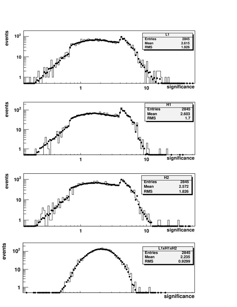
Figure 3: The significance distribution of the triple coincident WaveBurst events for individual detectors (L1, H1, H2) and the combined significance of their triple coincidences (L1xH1xH2) for the S2 data set. Solid histograms reflect the zero-lag events, while the points represent background (time-lag) events as produced with unphysical time shifts between the Livingston and Hanford detectors (and normalized to the S2 live-time). The change in the significance distribution for the individual detectors around significance equal to four is attributed to the onset of single pixel clusters (for which a higher threshold was applied).

V.3 $r$-statistic test

The $r$-statistic test Cadonati (2004) is applied as the final step of searching for gravitational wave event candidates. This test re-analyzes the raw (unprocessed) interferometer data around the times of coincident events identified by the WaveBurst ETG.

The fundamental building block in performing this waveform consistency test is the $r$-statistic, or the normalized linear correlation coefficient of two sequences, $\{x_{i}\}$ and $\{y_{i}\}$ (in this case, the two gravitational wave signal time series):

$$r=\frac{\sum_{i}(x_{i}-\bar{x})(y_{i}-\bar{y})}{\sqrt{\sum_{i}(x_{i}-\bar{x})^{2}}\sqrt{\sum_{i}(y_{i}-\bar{y})^{2}}},$$ (11)

where $\bar{x}$ and $\bar{y}$ are their respective mean values. This quantity assumes values between $-1$ for fully anti-correlated sequences and $+1$ for fully correlated sequences. For uncorrelated white noise, we expect the $r$-statistic values obtained for arbitrary sets of points of length $N$ to follow a normal distribution with zero mean and $\sigma=1/\sqrt{N}$. Any coherent component in the two sequences will cause $r$ to deviate from the above normal distribution. As a normalized quantity, the $r$-statistic does not attempt to measure the consistency between the relative amplitudes of the two sequences. Consequently, it offers the advantage of being robust against fluctuations of detector amplitude response and noise floor. A similar method based on this type of time-domain cross-correlation has been implemented in a LIGO search for gravitational waves associated with a GRB Mohanty et al. (2004); Abbott et al. (b) and elsewhere Astone et al. (2002a).

As will be described below, the final output of the $r$-statistic test is a combined confidence statistic which is constructed from $r$-statistic values calculated for all three pairs of interferometers. For each pair, we use only the absolute value of the statistic, $|r|$, rather than the signed value. This is because an astrophysical signal can produce either a correlation or an anticorrelation in the interferometers at the two LIGO sites, depending on its sky position and polarization. In fact, the $r$-statistic analysis was done using whitened (see below) but otherwise uncalibrated data, with an arbitrary sign convention. A signed correlation test using calibrated data would be appropriate for the H1-H2 pair, but all three pairs were treated equivalently in the present analysis.

The number of points $N$ considered in calculating the statistic in Eq. (11), or equivalently the integration time $\tau$, is the most important parameter in the construction of the $r$-statistic. Its optimal value depends in general on the duration of the signal being considered for detection. If $\tau$ is too long, the candidate signal is “washed out” by the noise when computing $r$. On the other hand, if it is too short, then only part of the coherent signal is included in the integration. Simulation studies have shown that most of the short-lived signals of interest to the LIGO burst search can be identified successfully using a set of three discrete integration times with lengths of 20, 50 and 100 ms.

Within its LIGO implementation, the $r$-statistic analysis first performs data “conditioning” to restrict the frequency content of the data to LIGO’s most sensitive band and to suppress any coherent lines and instrumental artifacts. Each data stream is first band-pass filtered with an 8th-order Butterworth filter with corner frequencies of 100 Hz and 1572 Hz, then down-sampled to a 4096 Hz sampling rate. The upper frequency of 1572 Hz was chosen in order to have 20 dB suppression at 2048 Hz and thus avoid aliasing. The lower frequency of 100 Hz was chosen to suppress the contribution of seismic noise; it also defines the lower edge of the frequency band for this gravitational wave burst search, since it is above the lower frequency limit of 64 Hz for WaveBurst triggers. The band-passed data are then whitened with a linear predictor error filter with a 10 Hz resolution trained on a 10 second period before the event start time. The filter removes predictable content, including lines that were stationary over a 10 second time scale. It also has the effect of suppressing frequency bands with large stationary noise, thus emphasizing transients Chatterji et al. (2004).

The next step in the $r$-statistic analysis involves the construction of all the possible $r$ coefficients given the number of interferometer pairs involved in the trigger, their possible relative time-delays due to their geographic separation, and the various integration times being considered. Relative time delays up to $\pm 10$ ms are considered for each detector pair, corresponding to the light travel time between the Hanford and Livingston sites. Future analyses will restrict the time delay to a much smaller value when correlating data from the two Hanford interferometers, to allow only for time calibration uncertainties. Furthermore, in the case of WaveBurst triggers with reported durations greater than the integration time $\tau$, multiple integration windows of that length are considered, offset from the reported start time of the trigger by multiples of $\tau/2$. For a given integration window indexed by $p$ (containing $N_{p}$ data samples), ordered pair of instruments indexed by $l,m$ $(l\neq m)$, and relative time delay indexed by $k$, the $r$-statistic value $|r^{k}_{plm}|$ is calculated. For each $p\,l\,m$ combination, the distribution of $|r^{k}_{plm}|$ for all values of $k$ is compared to the null hypothesis expectation of a normal distribution with zero mean and $\sigma=1/\sqrt{N_{p}}$ using the Kolmogorov-Smirnov test. If these are statistically consistent at the 95% level, then the algorithm assigns no significance to any apparent correlation in this detector pair. Otherwise, a one-sided significance and its associated logarithmic confidence are calculated from the maximum value of $|r^{k}_{plm}|$ for any time delay, compared to what would be expected if there were no correlation. Confidence values for all ordered detector pairs are then averaged to define the combined correlation confidence for a given integration window. The final result of the $r$-statistic test, $\Gamma$, is the maximum of the combined correlation confidence over all of the integration windows being considered. Events with a value of $\Gamma$ above a given threshold are finally selected.

The $r$-statistic implementation, filter parameters, and set of integration times were chosen based on their performance for various simulated signals. The single remaining parameter, the threshold on $\Gamma$, was tuned primarily in order to ensure that much less than one background event was expected in the whole S2 run, corresponding to a rate of O$(0.1)~{}\mu$Hz. Since the rate of WaveBurst triggers was approximately $15~{}\mu$Hz, as mentioned in Section V.2, a rejection factor of around 150 was required.

Table 1 shows the rejection efficiency of the $r$-statistic test for two thresholds on $\Gamma$ when the test is applied to white Gaussian noise (200 ms segments), to real S2 interferometer noise at randomly selected times (200 ms segments), and to the data at the times of time-lag (i.e., background) WaveBurst triggers in the S2 playground. In the first two cases, 200 ms of data was processed by the $r$-statistic algorithm, whereas in the latter case, the amount of data processed was determined by the trigger duration reported by WaveBurst. The table shows that random detector noise rarely produced a $\Gamma$ value above $3.0$, but the rejection factor for WaveBurst triggers was not high enough. A $\Gamma$ threshold of $4.0$ was ultimately chosen for this analysis, yielding an estimated rejection factor of $\sim 250$ for WaveBurst triggers.

Table 1: Percentage of S2 background events rejected by the $r$-statistic for two different thresholds on $\Gamma$.

Event Production	$\Gamma>3.0$	$\Gamma>4.0$
200 ms white Gaussian noise	$99.9992$%	$99.999996$%
200 ms real noise (random)	$99.89$%	$99.996$%
WaveBurst background events	$98.6\pm 0.5$%	$99.6\pm 0.3$%

As we will discuss in Section VIII, the $r$-statistic waveform consistency test with $\Gamma>4.0$ represents, for the waveforms we considered, a sensitivity that is equal to or better than that of the WaveBurst ETG. As a result of this, the false dismissal probability of the $r$-statistic test does not impair the efficiency of the whole pipeline.

VI Vetoes

We performed several studies in order to establish any correlation of the triggers produced by the WaveBurst search algorithm with environmental and instrumental glitches. LIGO records hundreds of auxiliary read-back channels of the servo control systems employed in the instruments’ interferometric operation as well as auxiliary channels monitoring the instruments’ physical environment. These channels can provide ways for establishing evidence that a transient is not of astrophysical origin, i.e., a glitch attributed to the instruments themselves and/or to their environment. Assuming that the coupling of these channels to a genuine gravitational wave burst is null (or below threshold within the context of a given analysis), such glitches appearing in these auxiliary channels may be used to veto the events that appear simultaneously in the gravitational wave channel.

Given the number of auxiliary channels and the parameter space that we need to explore for their analysis, an exhaustive a priori examination of all of them is a formidable task. The veto study was limited to the S2 playground data set and to a few tens of channels thought to be most relevant. Several different choices of filter and threshold parameters were tested in running the glitch finding algorithms. For each of these configurations, the efficiency of the auxiliary channel in vetoing the event triggers (presumed to be glitches), as well as the dead-time introduced by using that auxiliary channel as a veto, were computed and compared to judge the effectiveness of the veto condition.

Another important consideration in a veto analysis is to verify the absence of coupling between a real gravitational wave burst and the auxiliary channel, such that the real burst could cause itself to be vetoed. The “safety” (absence of such a coupling) of veto conditions was evaluated using hardware signal injections (described in section VIII), by checking whether the simulated burst signal imposed on the arm length appeared in the auxiliary channel. Only one channel, referred to as AS_I, in the L1 instrument derived from the antisymmetric port photodiode with a demodulation phase orthogonal to that of the gravitational wave channel, was found to be “unsafe” in this respect, containing a small amount of the injected signal.

None of the channels and parameters we examined yielded an obviously good veto (e.g., one with an efficiency of 20% or greater and a dead-time of no more than a few percent) to be used in this search. Among the most interesting channels was the one in the L1 instrument that recorded the DC level of the light out of the antisymmetric port of the interferometer, referred to as AS_DC. That channel was seen to correlate with the gravitational wave channel through a non-linear coupling with interferometer alignment fluctuations. A candidate veto based on this channel was shown to be able to reject $\sim 15$% of the triggers, but with a non-negligible dead-time of 5%. Finding no better option, we decided not to apply any a priori vetoes in this search, judging that the effect on the results would be insignificant.

Although none of the auxiliary channels studied in the playground data yielded a compelling veto, these studies provided experience applicable to examining any candidate gravitational wave event(s) found in the full data set. A basic principle established for the search was that a statistical excess of zero-lag event candidates (over the expected background) would not, by itself, constitute a detection; the candidate(s) would be subjected to further scrutiny to rule out any environmental or instrumental explanation that might not have been apparent in the initial veto studies. As will be described in the next section, one event did survive all the pre-determined cuts of the analysis but subsequent examination of auxiliary channels identified an environmental origin for the signal in the two Hanford detectors.

VII Signal and Background Rates

In the preceding section we described the methods that we used for the selection of burst events. These were applied to the S2 triple coincidence data set excluding the playground for a total of $239.5$ hours ($9.98$ days) of observation time. Every aspect of the analysis discussed from this point on will refer only to this data set.

VII.1 Event analysis

The WaveBurst analysis applied to the S2 data yielded 16 coincidence events (at zero-lag). The application of the $r$-statistic cut rejected 15 of them, leaving us with a single event that passed all the analysis criteria.

The background in this search is assumed to be due to random coincidences between unrelated triggers at the two LIGO sites. We have measured this background by artificially shifting the raw time series of the L1 instrument. As in our S1 search, we have chosen not to time-shift relative to each other the two Hanford instruments (H1, H2). Although we had no evidence of H1-H2 correlations in the S1 burst search, indications for such correlations in other LIGO searches exist Abbott et al. (2004d). A total of 46 artificial lags of the raw time series of the L1 instrument, at 5-second steps in the range [$-115$,$115$] seconds, were used in order to make a measurement of the accidental rate of coincidences, i.e., the background. This step size was much larger than the duration of any signal that we searched for and was also larger than the autocorrelation time-scale for the trigger generation algorithm applied to S2 data. This can be seen in Fig. 4 where a histogram of the time between consecutive events is shown for the double and their resulting triple coincidence WaveBurst zero-lag events before any combined significance or $r$-statistic cut is applied. These distributions follow the expected exponential form, indicating a quasi-stationary Poisson process. The background events generated in this way were also subjected to the $r$-statistic test in an identical way with the one used for the zero-lag events. Each time-shift experiment had a different live-time according to the overlap, when shifted, of the many non-contiguous data segments that were analyzed for each interferometer. Taking this into account, the total effective live-time for the purpose of measuring the background in this search was $391$ days, equal to $39.2$ times the zero-lag observation time.

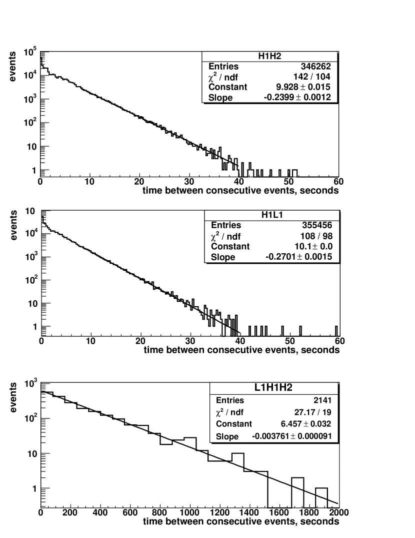
Figure 4: Time between consecutive WaveBurst events (prior to the application of the $r$-statistic test). The top two panels show the distributions for double-coincidence H1-H2 and H1-L1 triggers, respectively. The triple coincidence events, shown in the bottom panel, are reasonably well described by a Poisson process of constant mean. The exponential fits are performed for time delays greater than 4 s.

A plot of the measured background events found in each of the 46 time-lag experiments, before the application of the $r$-statistic, is shown in Fig. 5 as a function of the lag time. These numbers of events are corrected so that they all correspond to the zero-lag live-time. A Poisson fit can be seen in the adjacent panel; the fit describes the distribution of event counts reasonably well.

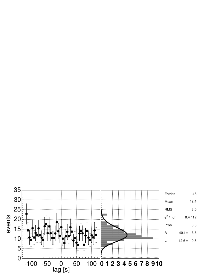
Figure 5: WaveBurst event count (prior to the $r$-statistic test) versus lag time (in seconds) of the L1 interferometer with respect to H1 and H2. The zero-lag measurement, i.e., the only coincidence measurement that is physical, is also shown. Due to the fragmentation of the data set, each time-lag has a slightly different live-time; for this reason, the event count is corrected so that they all correspond to the zero-lag live-time. A projection of the event counts to a one-dimensional histogram with a Poisson fit is also shown in the adjacent panel.

Figure 6 shows a histogram of the $\Gamma$ values, i.e., the multi-interferometer combined correlation confidence, for the zero-lag events. The normalized background distribution, estimated from time-lag coincidences, is shown for comparison. One zero-lag event passed the requirement $\Gamma>4$ that we had chosen based on the playground data; this event will be discussed in the following subsection. Only two time-lag coincidences above this $\Gamma$ threshold were found among all 46 time lags. With such low statistics, the rate and distribution of the background for large $\Gamma$ is poorly known, but we can get an approximate measure of the significance of the zero-lag event by comparing it to the cumulative mean background rate with $\Gamma>4$, which is roughly $0.05$ events for the same observation time. Thus, the chance of having found such a background event in the zero-lag sample is roughly 5%. Table 2 summarizes the number of events and corresponding rates before and after the application of the $r$-statistic. The background estimates reported in the table are normalized to the same live-time as for the zero-lag coincidence measurement.

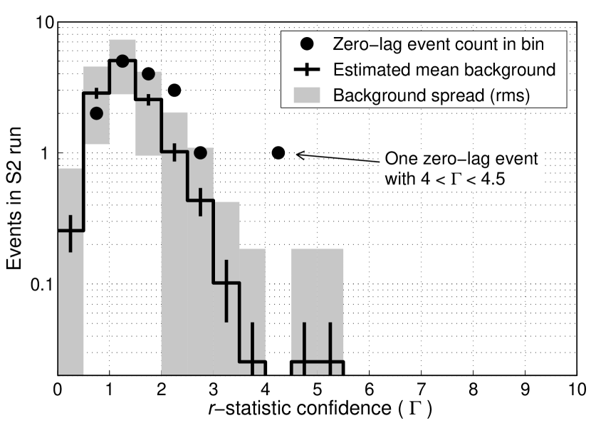
Figure 6: Circles: histogram of $r$-statistic confidence value ($\Gamma$) for zero-lag events passing the WaveBurst analysis. Stair-step curve: mean background per bin, estimated from time lags, for an observation time equal to that of the zero-lag analysis. The black error bars indicate the statistical uncertainty on the mean background. The shaded bars represent the expected root-mean-square statistical fluctuations on the number of background events in each bin.

Table 2: Event statistics for the S2 burst search. The expected numbers of background events are normalized to the live-time of the zero-lag analysis.

WaveBurst	events in $239.5$ hours ($9.98$ days)	rate
	Before $r$-statistic test
Coincidences	16	$18.6\;\mu$Hz
Background	12.3	$14.3\pm 0.7\;\mu$Hz
	After $r$-statistic test
Coincidences	1	$1.2\;\mu$Hz
Background	0.05	$0.06\pm 0.04\;\mu$Hz

Sources of systematic errors may arise in the choices we have made on how to perform the time-lag experiments, namely the choice of step and window size as well as the time-lag method by itself. We have performed time-lag experiments using different time steps, all of which yielded statistically consistent results. The one-sigma systematic uncertainty from the choice of step size is estimated to be less than 0.04 events with $\Gamma>4$.

VII.2 Examination of the surviving event candidate

The single event in the triple coincidence data set that survived all previously described analysis cuts barely passed the WaveBurst combined significance and $r$-statistic thresholds. An examination of the event parameters estimated by WaveBurst revealed that the three instruments recorded low frequency signals in the $\sim 135$ Hz range and with comparable bandwidths, although WaveBurst provides only a rough estimate of the dominant frequency of an event candidate. The signal $h_{\mathrm{rss}}$ strengths in the two Hanford detectors were in the $6\times 10^{-20}-10^{-19}$ Hz^-1/2 range, well above the instruments’ typical noise in this band, while for the Livingston detector, $h_{\mathrm{rss}}$ was at the $2.7\times 10^{-21}$ Hz^-1/2 level, much closer to the noise floor of the instrument.

Given the low estimated probability of this event being due to a random triple coincidence, it was treated as a candidate gravitational wave detection and was therefore subjected to additional scrutiny. In particular, the auxiliary interferometric and environmental monitoring channels were examined around the time of the event to check for an interferometer malfunction or an environmental cause. The investigation revealed that the event occurred during a period of strongly elevated acoustic noise at Hanford lasting tens of seconds, as measured by microphones placed near the interferometers. The effects of environmental influences on the interferometers were measured in a special study during the S2 run by intentionally generating acoustic and other environmental disturbances and comparing the resulting signals in the gravitational wave and environmental monitoring channels. These coupling measurements indicated that the acoustic event recorded on the microphones could account for the amplitude and frequency of the signal in the H1 and H2 gravitational wave channels at the time of the candidate event. On this basis, it was clear that the candidate event should be attributed to the acoustic disturbance and not to a gravitational wave.

The source of the acoustic noise appears to have been an aircraft. Microphone signals from the five Hanford buildings exhibited Doppler frequency shifts in a sequence consistent with the overflight of an airplane roughly paralleling the X arm of the interferometers, on a typical approach to the nearby Pasco, Washington airport. Similar signals in the microphone and gravitational wave channels at other times have been visually confirmed as over-flying airplanes.

No instrumental or environmental cause was identified for the signal in the Livingston interferometer at the time of the candidate event, but that signal was much smaller in amplitude and was consistent with being a typical fluctuation in the Livingston detector noise, accidentally coincident with the stronger signals in the two Hanford detectors.

Because of the sensitivity of the interferometers to the acoustic environment during S2, a program to reduce acoustic coupling was undertaken prior to S3. The acoustic sensitivities of the interferometers were reduced by 2 to 3 orders of magnitude by addressing the coupling mechanisms on optics tables located outside of the vacuum system, and by acoustically isolating the main coupling sites.

VII.3 Propeller-airplane acoustic veto

Given the clear association of the surviving event with an acoustic disturbance, we tracked the power in a particular microphone channel, located in the LIGO Hanford corner station, over the entire S2 run. We defined a set of time intervals with significantly elevated acoustic noise by setting a threshold on the power in the 62–100 Hz band—where propeller airplanes are observed to show up most clearly—averaged over one-minute intervals. The threshold was chosen by looking at the distribution over the entire S2 run, and was far below the power at the time of the “airplane” outlier event discussed above. Over the span of the run, $0.7$% of the data was collected during times of elevated acoustic noise as defined in this way. Eliminating these time intervals removes the zero-lag outlier as well as the time-lag event with the largest value of $\Gamma$, while having only a slight effect on the rest of the background distribution, as shown in Fig. 7. We conclude that acoustic disturbances from propeller airplanes contribute a small but non-negligible background if this veto is not applied.

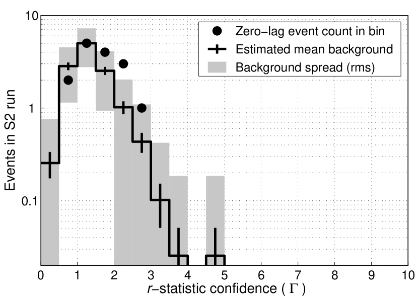
Figure 7: Circles: histogram of $r$-statistic confidence value ($\Gamma$) for zero-lag events passing the WaveBurst analysis and surviving the acoustic veto. The background estimated from time-lag events surviving the acoustic veto is shown in the same manner as in Fig. 6.

VII.4 Rate limit

We now use the results of this analysis to place a limit on the average rate (assuming a uniform distribution over time) of gravitational wave bursts that are strong enough to be detected reliably by our analysis pipeline. The case of somewhat weaker signals, which are detectable with efficiency less than unity, will be considered in the next section.

Our intention at the outset of this analysis was to calculate a frequentist 90% confidence interval from the observation time, number of observed candidate events, and estimated background using the Feldman-Cousins Feldman and Cousins (1998) approach. Although this procedure could yield an interval with a lower bound greater than zero, we would not claim the detection of a gravitational wave signal based on that criterion alone; we would require a higher level of statistical significance, including additional consistency tests. Thus, in the absence of a detection, our focus is on the upper bound of the calculated confidence interval; we take this as an upper limit on the event rate.

The actual outcome of our analysis presented us with a dilemma regarding the calculation of a rate limit. Our pipeline was designed to perform a “blind” upper limit analysis, with all choices about the analysis to be based on playground data which was excluded from the final result; following this principle, the “emergent” acoustic veto described above should be disallowed (since it was developed in response to the candidate event which passed all of the initial cuts), and the upper bound should be calculated based on a sample of one candidate event. On the other hand, it seemed unacceptable to ignore the clear association of that event with a strong acoustic disturbance and to continue to treat it as a candidate gravitational wave burst. We decided to apply the acoustic veto, reducing the observation time by $0.7$% and calculating an upper limit based on a final sample containing no events. However, any decision to alter the analysis procedure based on information from the analysis must be approached with great caution and an awareness of the impact on the statistics of the result. In particular, a frequentist confidence interval construction which has been designed to give 90% minimum coverage for an ordinary (unconditional) analysis procedure can yield less than 90% coverage if it is blindly used in a conditional analysis involving an emergent veto, due to the chance that a real gravitational wave burst could be vetoed, and due to the fact that the background would be mis-estimated. In the present analysis, we know that the chance of a gravitational wave burst being eliminated by the acoustic veto described above is only $0.7$%; however, we must consider the possibility that there are other, “latent” veto conditions which are not associated with any events in this experimental instance but which might be adopted to veto a gravitational wave burst in case of a chance coincidence.

It is impossible to enumerate all possible latent veto conditions without an exhaustive examination of auxiliary channels in the full data set. Judging from our experience with examining individual event candidates and potential veto conditions in the playground data set, we believe that there are few possible veto conditions with sufficiently low dead-time and a plausible coupling mechanism (like the acoustic veto) to be considered. Nevertheless, we have performed Monte Carlo simulations to calculate frequentist coverage for various conditional limit-setting procedures under the assumption that there are many latent vetoes, with a variety of individual dead-times and with a net combined dead-time of 35%. A subset of eight latent vetoes with individual dead-times less than 5%, sufficiently low that we might adopt the veto if it appeared to correlate with a single gravitational-wave event, had a combined dead-time of 12%. Veto conditions with larger dead-times would be considered only if they seemed to explain multiple event candidates to a degree unlikely to occur by chance.

The simulations led us to understand that we can preserve the desired minimum coverage (e.g., 90%) by assigning a somewhat larger interval when an emergent veto has been applied. This is a means of incorporating the information that an observed event is probably due to the environmental disturbance identified by the veto, without assuming that it is certainly due to the environmental disturbance and simply applying the veto. The resulting upper limit is looser than what would be obtained by simply applying the veto. Among a number of possible ways to assign such an interval, we choose to use the Feldman-Cousins interval calculation with an input confidence level somewhat greater than our target coverage and with the background taken to be zero. Taking the background to be zero provides some necessary conservatism since we have not sought vetoes for the time-lag coincidences from which the background was originally estimated, but this has little effect on the result since the background rate is low.

According to the simulations, using a confidence level of 92% in the Feldman-Cousins upper limit calculation after adopting an emergent veto is sufficient to ensure an actual minimum coverage of greater than 90%, and using a confidence level of 96% is sufficient to ensure an actual minimum coverage of greater than 95%. The resulting rate limits for strong gravitational wave bursts are presented in Table 3. The upper limit at 90% confidence, $0.26$ events per day, represents an improvement over the rate limit from our S1 result Abbott et al. (2004c) by a factor of 6. As will be described in the following section, the present analysis also is sensitive to much weaker bursts than the S1 analysis was.

Table 3: Upper limits on the rate of strong gravitational wave bursts for two different frequentist confidence levels. The method used to calculate these limits is described in the text.

Confidence level	Upper limit
90%	$0.26$ events/day
95%	$0.33$ events/day

VIII Efficiency of the Search

VIII.1 Target waveforms and signal generation

In order to estimate the sensitivity of the burst analysis pipeline, we studied its response to simulated signals of various waveform morphologies and strengths. The simulated signals were prepared in advance, then “injected” into the S2 triple coincidence data set by using software to add them to the digitized time series that had been recorded by the detectors Klimenko et al. (2004b). The times of the simulated signals were chosen pseudo-randomly, uniformly covering the S2 triple coincidence data set with an average separation of one minute and a minimum separation of 10 seconds. The modified data streams were then re-analyzed using the same analysis pipeline.

Several ad hoc and astrophysically motivated waveforms were selected for injections:

• sine-Gaussian waveforms of the form $h(t+t_{0})=h_{0}\sin(2\pi f_{0}t)\exp(-t^{2}/\tau^{2})$, where $\tau$ was chosen according to $\tau=$Q$/(\sqrt{2}\pi f_{0})$ with Q=8.9, and $f_{0}$ assumed the value of 100, 153, 235, 361, 554, and 849 Hz;

• Gaussian waveforms of the form $h(t+t_{0})=h_{0}\exp(-t^{2}/\tau^{2})$ and with $\tau$ equal to 0.1, 0.5, 1.0, 2.5, 4.0 and 6.0 ms;

• waveforms resulting from numerical simulations of core collapse supernovae that are available in the literature Zwerger and Müller (1997); Dimmelmeier et al. (2001); Ott et al. (2004);

• binary black hole merger waveforms as described in Baker et al. (2002); ast and for total system masses of 10, 30, 50, 70 and 90 solar masses.

The sine-Gaussian and Gaussian waveforms were chosen to represent the two general classes of short-lived gravitational wave bursts of narrow-band and broad-band character respectively. The supernovae and binary black hole merger waveforms were adopted as a more realistic model for gravitational wave bursts.

In order to ensure self-consistent injections which would accurately test the coincidence criteria in the pipeline, we took into account the exact geometry of the individual LIGO detectors with respect to the impinging gravitational burst wavefront. A gravitational wave burst is expected to be comprised of two waveforms $h_{+}(t)$ and $h_{\times}(t)$ which represent its two polarizations, conventionally defined with respect to the polarization of the source. The signal produced on the output of a LIGO detector $h_{det}(t)$ is a linear combination of these two waveforms,

$$h_{det}(t)=F_{+}h_{+}(t)+F_{\times}h_{\times}(t),$$ (12)

where $F_{+}$ and $F_{\times}$ are the antenna pattern functions Thorne (1987); Saulson (1994). The antenna pattern functions depend on the source location on the sky (spherical polar angles $\theta$ and $\phi$) and the wave’s polarization angle $\psi$. The source coordinates $\theta$ and $\phi$ were chosen randomly so that they would appear uniformly distributed on the sky. For every source direction the simulated signals were injected with the appropriate relative time delay corresponding to the geometric separation of the two LIGO sites. For the two ad hoc waveform families (sine-Gaussian, Gaussian) as well as for the supernovae ones, a linearly polarized wave was assumed with a random polarization angle. The binary black hole merger waveforms come with two polarizations Baker et al. (2002) and both were taken into account.

For the supernovae waveforms the inclination of the source with respect to the line of sight was taken to be optimal (ninety degrees), so that the maximum gravitational wave emission is in the direction of the Earth. For the binary black hole merger case we used the same $h_{\mathrm{rss}}$ amplitude in the two polarizations thus corresponding to an inclination of 59.5 degrees. Of course, a real population of astrophysical sources would have random inclinations, and the wave amplitude at the Earth would depend on the inclination as well as the intrinsic source strength and distance. Our injection approach is in keeping with our intent to express the detection efficiency in terms of the gravitational wave amplitude reaching the Earth, not in terms of the intrinsic emission by any particular class of sources (even though some of the waveforms we consider are derived from astrophysical models). For a source producing radiation in only one polarization state, a change in the inclination simply reduces the amplitude at the Earth by a multiplicative factor. However, a source which emits two distinct polarization components produces a net waveform at the Earth which depends nontrivially on inclination angle; thus, our fixed-inclination injections of black hole merger waveforms can only be considered as discrete examples of such signals, not as representative of a population. In any case, the waveforms we use are only approximations to those expected from real supernovae and black hole mergers.

VIII.2 Software injection results

In order to add the aforementioned waveforms to the raw detector data, their signals were first digitized at the LIGO sampling frequency of 16384 Hz. Their amplitudes defined in strain dimensionless units were converted to units of ADC counts using the response functions of the detectors determined from calibration González et al. (2004). The resulting time series of ADC($t$) were then added to the raw detector data and were made available to the analysis pipeline. In analyzing the injection data, every aspect of the analysis pipeline that starts with single-interferometer time series ADC($t$) and ends with a collection of event triggers was kept identical to the one that was used in the analysis of the real, interferometric data, including the acoustic veto. For each of the four waveform families we introduced earlier in this section, a total of approximately 3000 signals were injected into the three LIGO detectors, uniformly distributed in time over the entire S2 data set that was used for setting the rate bound. As in our S1 signal injection analysis, we quantify the strength of the injected signals using the root-sum-square (rss) amplitude at the Earth (i.e., without folding in the antenna pattern of a detector) defined by

$$h_{\mathrm{rss}}\equiv\sqrt{\int(|h_{+}(t)|^{2}+|h_{\times}(t)|^{2})\,dt}~{}.$$ (13)

This is a measure of the square root of the signal “energy” and it can be shown that, when divided by the detector spectral noise, it approximates the signal-to-noise ratio that is used to quantify the detectability of a signal in optimal filtering. The quantity $h_{\mathrm{rss}}$ has units of Hz^-1/2 and can thus be directly compared to the detector sensitivity curves, as measured by power spectral densities over long time scales. The pixel and cluster strength quantities calculated by the WaveBurst ETG are monotonic functions of the $h_{\mathrm{rss}}$ of a given signal. The $h_{\mathrm{rss}}$ amplitudes of the injected signals were chosen randomly from 20 discrete logarithmically-spaced values in order to map out the detection efficiency as a function of signal strength.

The efficiency of the analysis pipeline is defined as the fraction of injected events which are successfully detected. The software injections exercised a range of signal strengths that allowed us to measure (in most cases) the onset of efficiency up to nearly unity. Efficiency measurements between $0.01$ and $0.99$ were fitted with an asymmetric sigmoid of the form

$$\epsilon(h_{\mathrm{rss}})=\frac{1}{1+\left(\frac{h_{\mathrm{rss}}}{h_{\mathrm{mid}}}\right)^{\alpha\left(1+\beta\tanh(h_{\mathrm{rss}}/h_{\mathrm{mid}})\right)}}\,,$$ (14)

where $h_{\mathrm{mid}}$ is the $h_{\mathrm{rss}}$ value corresponding to an efficiency of $0.5$, $\beta$ is the parameter that describes the asymmetry of the sigmoid (with range $-1$ to $+1$), and $\alpha$ describes the slope. The analytic expressions of the fits were then used to determine the signal strength $h_{\mathrm{rss}}$ for which an efficiency of 50%, 90% and 95% was reached.

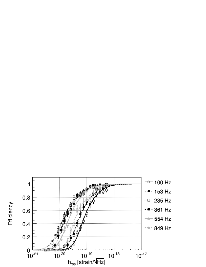
Figure 8: Detection efficiency of the analysis pipeline as a function of the signal strength for sine-Gaussian waveforms of Q=8.9 and central frequencies of 100, 153, 235, 361, 554 and 849 Hz. The efficiencies plotted reflect averaging over random sky positions and polarization angles for injections covering the entire S2 data set. The $x$ axis reflects the $h_{\mathrm{rss}}$ as defined in equation 13.

In Fig. 8 we show the efficiency curves, i.e., the efficiency versus signal strength (at the Earth) of our end-to-end burst search pipeline for the case of the six different sine-Gaussian waveforms we have introduced earlier in this section. As described in the previous subsection, these efficiency curves reflect averaging over random sky positions and polarization angles. As expected given the instruments’ noise floor (see Fig. 1), the best sensitivity is attained for sine-Gaussians with a central frequency of 235 Hz; for this signal type, the required strength in order to reach 50% efficiency is $h_{\mathrm{rss}}=$1.5$\times 10^{-20}$ Hz^-1/2, which is roughly a factor of 20 above the noise floor of the least sensitive LIGO instrument at 235 Hz during S2. In Fig. 9 we show the same curves for the Gaussian family of waveforms we considered. The 6 ms Gaussian presents the worst sensitivity because most of its signal power is below 100 Hz. The maximum $h_{\mathrm{rss}}$ used for the Gaussian injections was $1.32\times 10^{-18}$ Hz^-1/2; we cannot rely on the fitted curves to accurately extrapolate the efficiencies much beyond that $h_{\mathrm{rss}}$. The sensitivity of this search to $h_{\mathrm{rss}}$ for these two families of waveforms is summarized in Table 4.

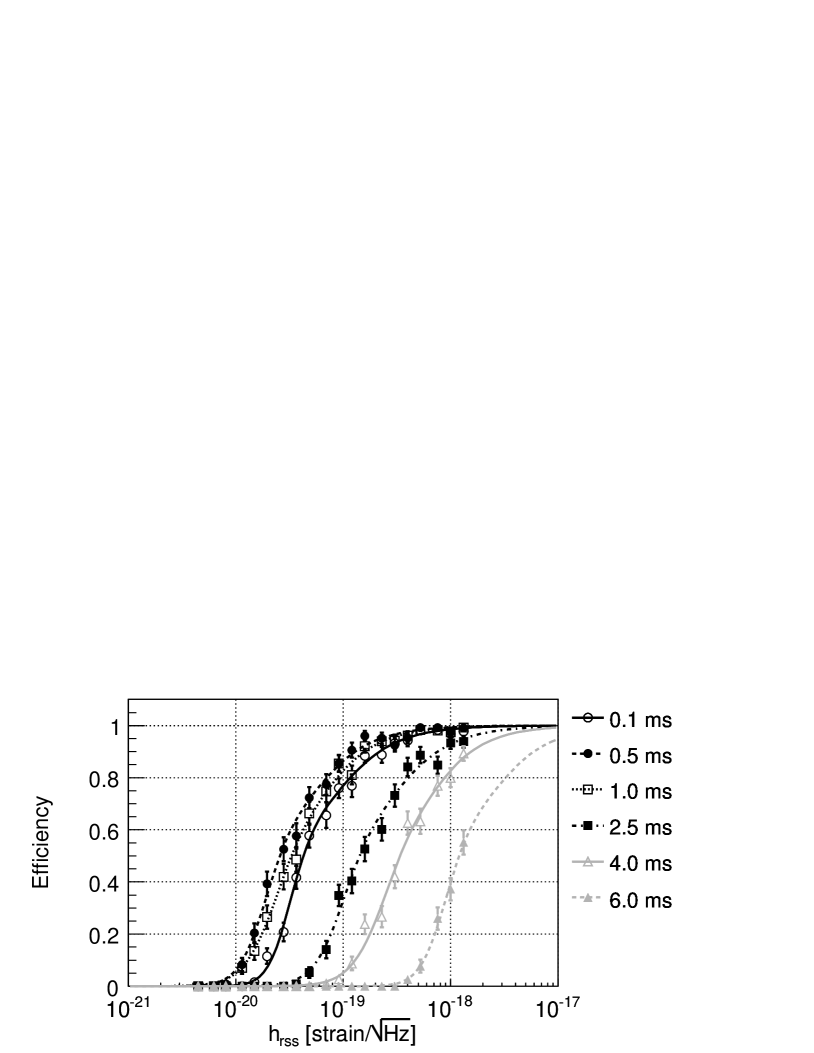
Figure 9: Same plot as in Fig. 8 but for Gaussian injections of $\tau=$0.1, 0.5, 1.0, 2.5, 4.0 and 6.0 ms.

Table 4: Summary of the S2 pipeline $h_{\mathrm{rss}}$ (from equation 13) sensitivity to ad hoc waveforms in units of $10^{-20}$ Hz^-1/2. These values are averages over random sky positions and signal polarizations. The injections did not span a wide enough range of amplitudes to accurately determine the 95% efficiency value for the $\tau$=$4.0$ ms Gaussian, nor the 90% and 95% efficiency values for the $\tau$=$6.0$ ms Gaussian.

	50%	90%	95%
sine-Gaussian $f_{0}$=100 Hz	8.2	33	53
sine-Gaussian $f_{0}$=153 Hz	5.5	24	40
sine-Gaussian $f_{0}$=235 Hz	1.5	7.6	13
sine-Gaussian $f_{0}$=361 Hz	1.7	8.2	14
sine-Gaussian $f_{0}$=554 Hz	2.3	10	17
sine-Gaussian $f_{0}$=849 Hz	3.9	20	34
Gaussian $\tau$=0.1 ms	4.3	21	37
Gaussian $\tau$=0.5 ms	2.6	13	22
Gaussian $\tau$=1.0 ms	3.3	16	26
Gaussian $\tau$=2.5 ms	14	75	130
Gaussian $\tau$=4.0 ms	34	154	—
Gaussian $\tau$=6.0 ms	121	—	—

VIII.3 Signal parameter estimation

The software signal injections we just described provide a good way of not only measuring the efficiency of the search but also benchmarking WaveBurst’s ability to extract the signal parameters. An accurate estimation of the signal parameters by a detection algorithm is essential for the successful use of time and frequency coincidence among candidate triggers coming from the three LIGO detectors.

We compare the central time of a WaveBurst event (section V) with the known central time of the signal injection. For each of the two ad hoc waveform families considered so far, as well as for each of the astrophysical waveforms we will discuss in section IX, WaveBurst is able to resolve the time of the event on the average with a systematic shift of less than 3 ms and with a standard deviation of the same value. In Fig. 10 we show a typical plot of the timing error for the case of all the sine-Gaussian injections we injected in the software simulations and for the three LIGO instruments together. The apparent deviation from zero has a contribution coming from the calibration phase error. Another contribution comes from the fact that the detected central time is based on a finite time-frequency volume of the signal’s decomposition which is obtained after thresholding. It remains however well within our needs for a tight time coincidence between interferometers. For the same type of signals, we list in Table 5 the reconstructed versus injected central frequency. The measurements are consistent within the signal bandwidth.

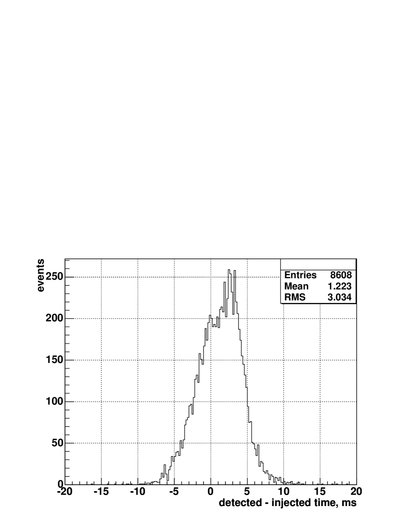
Figure 10: Timing error of the WaveBurst algorithm in the three LIGO instruments during S2 when sine-Gaussian injections of varying frequency and strength were injected. For comparison, the time separation between the two LIGO sites is 10 ms and the coincidence time window used in this analysis is 20 ms.

Table 5: Central frequency reconstruction for Q=8.9 sine-Gaussian injections.

Injected	Mean of detected	Standard deviation of
frequency (Hz)	frequency (Hz)	detected frequency (Hz)
100	98.4	3.9
153	159.5	4.4
235	242.7	14.2
361	363.7	14.0
554	544.3	17.0
849	844.9	21.4

The WaveBurst algorithm estimates the signal strength from the measured excess power in the cluster pixels, expressed as $h_{\mathrm{rss}}$ as in equation 13 but with the integrand being the antenna-pattern-corrected $h_{det}(t)$ given by equation 12 rather than the intrinsic $h(t)$ of the gravitational wave. Figure 11 shows that this quantity is slightly overestimated on average, particularly for weak signals. Several factors contribute to mis-estimation of the signal strength. WaveBurst limits the signal $h_{\mathrm{rss}}$ integration to within the detected time-frequency volume of an event and not over the entire theoretical support of a signal. Errors in the determination of the signal’s time-frequency volume due to thresholding may lead to systematic uncertainties in the determination of its strength. The $h_{\mathrm{rss}}$ shown in Fig. 11 also reflects the folding of the measurements from all three LIGO instruments and thus it is affected by calibration errors and noise fluctuations in any instrument. Our simulation analysis has shown that the detected signal’s $h_{\mathrm{rss}}$ is the quantity most sensitive to detector noise and its variability; for this reason, it is not used in any step of the analysis either as part of the coincidence analysis or for the final event selection.

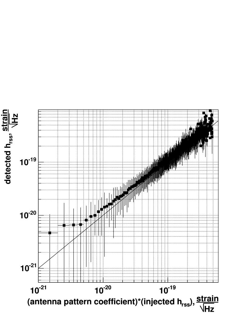
Figure 11: Detected versus injected root-sum-square (rss) signal strength for Q=8.9 sine-Gaussian injections. The vertical bars indicate one-sigma spread of the reconstructed values.

VIII.4 Hardware injection results

During the S2 data taking, as well as shortly before and after it, several run intervals were designated for hardware signal injections. These injections were intended to address any instrumental issues, including calibrations, and provide a robust end-to-end test of LIGO’s data analysis pipelines. They also provided an important tool for establishing the “safety” of the veto analysis, i.e., the absence of any couplings between a real gravitational wave burst and the auxiliary channels we considered as potential vetoes (section VI). An arbitrary function generator connected to the mirror position actuators provided the capability of exciting the mirrors according to a simulated gravitational wave pattern. The waveforms injected through this hardware calibration included several of the ones described in the target waveform section above. The signals were injected into all three LIGO instruments at identical times, without attempting to mock up the relative time delays and amplitudes that would be produced by a source at a particular position in the sky. Thus the coincidence analysis, using the end-to-end pipeline invoked in the analysis of the real data alone as well as with software injections, was not fully appropriate for the hardware injections. We have restricted ourselves to examining the performance of the LIGO instruments and of the WaveBurst ETG in detecting these events and reconstructing their signal parameters using each individual detector. Both the time and frequency reconstruction by the WaveBurst algorithm on these hardware-injected signals is consistent with our software injections and within our expectations.

VIII.5 Error analysis

The largest source of systematic error in the efficiency of this search is uncertainty in the absolute calibration of the detectors. Several contributions to this uncertainty have been considered González et al. (2004). Systematic uncertainties are less than 12% for L1, 5% for H1, and 6% for H2 over the frequency band used in this analysis. The calibration at any given point in time is subject to an additional uncertainty from detector noise affecting the measurement of the amplitude of the calibration lines. These random errors were especially large near the beginning of the run, when the H1 and L1 calibration lines were rather weak. However, the efficiency of the search, averaged over the run, is insensitive to these random errors. The overall systematic uncertainty on the triple-coincidence efficiency is a combination of the individual systematic uncertainties which depends on the relative sensitivities of the detectors, with the least sensitive detector having the greatest influence. As shown in Fig. 1, H2 was the least sensitive detector at low frequencies while H1 was the least sensitive at high frequencies. The net uncertainty in the efficiency is estimated to be less than 8% at all frequencies.

No significant systematic error is attributed to the procedure we followed in order to perform the efficiency measurement. The various signal morphologies were superimposed over the entire S2 data sample and its full range of detector behavior. The statistical error attributed to the finite number of simulations used for the efficiency measurement is reflected in the goodness of the sigmoid-like fits and is estimated to be less than 5%. The efficiency measurement was performed in multiple slightly-varying ways all of which yielded results within one standard deviation. These variations included different sampling of the S2 data set, different versions of the calibration constants, and different number and placement of the signal injections.

Combining all uncertainties, we estimate our efficiency to any given signal morphology to be accurate at the 10% level or better.

IX Search Results

IX.1 Rate versus strength upper limit

As we have seen in section VII, using the zero-lag and background rate measurements we set an upper bound on the rate of gravitational wave bursts at the instruments at the level of $0.26$ events per day at the 90% confidence level. We will now use the measurement of the efficiency of the search as described in the previous section in order to associate the above rate bound with the strength of the gravitational wave burst events. This is the rate versus strength interpretation that we introduced in our previous search for bursts in LIGO using the S1 data Abbott et al. (2004c).

The rate bound of our search as a function of signal strength $h_{\mathrm{rss}}$ is given by

$$R(h_{\mathrm{rss}})=\frac{\eta}{\epsilon(h_{\mathrm{rss}})}$$ (15)

where the numerator $\eta$ is the upper bound on the rate of detectable signal events at a given confidence level (Sec. VII.4) and the denominator is the fractional efficiency for signals of strength $h_{\mathrm{rss}}$ (at the Earth). This rate versus strength interpretation makes the same assumptions on the signal morphology and origin as the ones that enter in the determination of the efficiency. In Fig. 12 we show the rate versus strength upper limit for the sine-Gaussian and Gaussian waveform families. For a given signal strength $h_{\mathrm{rss}}$ these plots give the upper limit at the 90% confidence level on the rate of burst events at the instruments with strength equal to or greater than $h_{\mathrm{rss}}$. In that sense, the part of the plot above and to the right of these curves defines the region of signal strength-rate excluded by this search at 90% confidence level. As one would expect, for strong enough signals the efficiency of the search is 1 for all the signal morphologies: this part of the plot remains flat at a level that is set primarily by the observation time of this search. For weaker signals the efficiency decreases and the strength-rate plot curves up. Eventually, as the efficiency vanishes the rate limit reaches infinity asymptotically. These curves for the various waveforms are not identical, as the detailed trailing off of the efficiency is dependent on the waveform. The exclusion rate-strength plots obtained from the S2 analysis represent a significant improvement with respect to the S1 result Abbott et al. (2004c). As already noted in section VII, the horizontal part of the plot determined by the observation time is improved by a factor of 6 while the sensitivity-limited curved part of it reflects an improvement in the efficiency of a factor of 17 or better, depending on the waveform morphology.

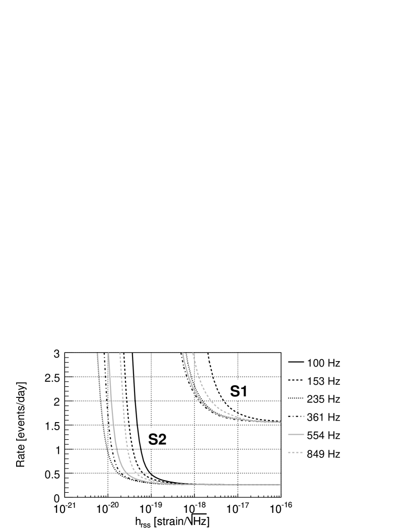
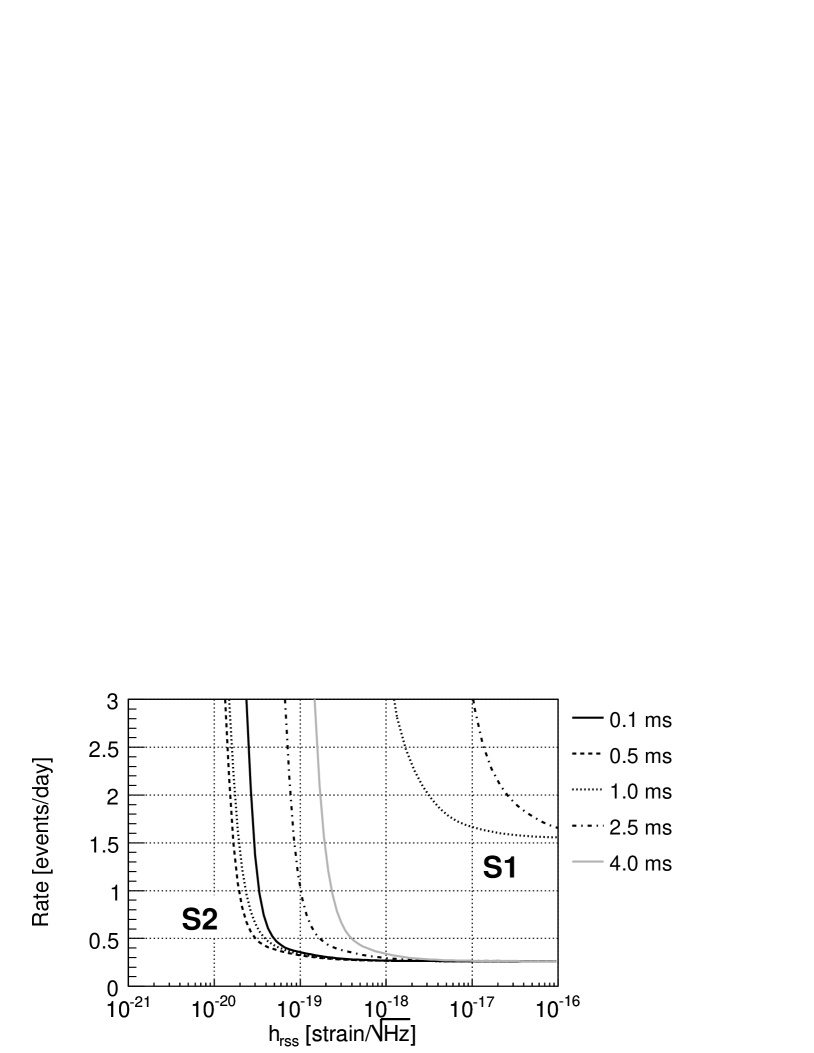
Figure 12: Rate versus $h_{\mathrm{rss}}$ exclusion plots at the 90% confidence level derived from the LIGO burst search using the S2 data. The top plot corresponds to burst events modeled by sine-Gaussians of Q=8.9 and frequencies ranging from 100 Hz to 849 Hz, while the bottom plot corresponds to ones events modeled by Gaussians of the $\tau$’s shown. For comparison, the corresponding curves resulting from the S1 analysis are superimposed.

IX.2 Astrophysical waveforms

As mentioned in the introduction, potential sources of gravitational wave bursts targeted in this search include core collapse supernovae, merging compact binaries (neutron stars and/or black holes) and gamma ray bursts. In recent years there has been much effort devoted to predicting gravitational wave burst waveforms from astrophysical sources, generally relying on detailed numerical and approximation methods. Our search is designed to be sensitive to a broad range of short-duration bursts, so we wish to evaluate how it performs for plausible astrophysical signals suggested by certain models. As part of our signal simulation analysis for this search, we focus in particular on the case of the core collapse of rapidly spinning massive stars  Zwerger and Müller (1997); Dimmelmeier et al. (2001); Ott et al. (2004), and of binary black hole mergers Baker et al. (2002, 2004); ast .

The core collapse simulations employ detailed hydrodynamical models in two dimensions, enforcing axisymmetry of the rotating star throughout its evolution. The core collapse is initiated artificially (e.g., through a change in the adiabatic index of the core material Zwerger and Müller (1997)). An accelerating quadrupole moment is calculated in 2D from the distribution and flow of matter during the collapse, from which the gravitational wave signal is derived. The rapid spinning of the progenitor star may produce multiple bounces of the dense core, which is reflected in the waveform of the emitted waves. Simple models of the differential rotation of material in the star also lead to significant differences in the resulting waveforms. Relativistic effects Dimmelmeier et al. (2001), if included, serve to effectively “stiffen” the core, shifting the waves to higher frequencies and shorter durations. The simulation is followed through the core collapse phase when most of the gravitational wave signal is produced; it need not be continued through to the explosion of the outer layers (and indeed, these simulations may not produce such explosions). The simulations attempt to sample the space of important parameters (progenitor star angular momentum, differential angular momentum versus radius, density versus radius, adiabatic index of the core, etc.), resulting in collections of waveforms with widely varying morphologies; but of course the actual distributions of such parameters are poorly known. In ref. Ott et al. (2004) the authors employ updated progenitor models and nuclear equation of state. For the studies described here, we make use of 78 waveforms supplied in ref. Zwerger and Müller (1997), 26 from ref. Dimmelmeier et al. (2001), and 72 from ref. Ott et al. (2004). We emphasize that we are studying these waveforms only as a guide for evaluating our search algorithm; we do not rely on accurately modelling a realistic population of progenitor stars.

The binary black hole merger waveforms are taken from the Lazarus project Baker et al. (2002, 2004); ast , which combines numerical simulation of the vacuum Einstein equations for the most significantly nonlinear part of the interaction with close-limit perturbation theory for the late-time dynamics. The authors in Baker et al. (2002, 2004); ast generate waveforms from simulations of equal mass binary black holes with no intrinsic spin starting from near the innermost stable circular orbit following a binary black hole inspiral. It should be kept in mind that these waveforms include the ringdown phase of the binary system and would naturally occur after an inspiral waveform, which is searched for using matched filtering techniques Abbott et al. (2004b); ref (a).

In all of these models, the simulations and calculations predict gravitational wave bursts with time durations ranging from a fraction of a millisecond to tens or hundreds of milliseconds and with a significant fraction of their power in LIGO’s most sensitive frequency band (100–1100 Hz). This observation motivates the choice of parameters for the sine-Gaussian and Gaussian waveforms used to optimize and evaluate the efficiency for our search pipeline, as discussed in section VIII. After tuning our pipeline algorithms using these ad hoc waveforms, we evaluate the efficiency for our search to detect the waveforms predicted from the astrophysical simulations. The amplitudes of these waveforms are predicted by the simulations, so that in addition to evaluating the efficiency as a function of $h_{\mathrm{rss}}$ (at the Earth), we can also present them as a function of distance to the source (for a particular source inclination). We have evaluated the efficiency versus actual distance, averaged over source directions and polarizations, assuming an isotropic distribution in source direction. This assumption becomes invalid for supernova progenitors in the Galactic disk, when the LIGO detectors become sensitive to supernovae at distances greater than the disk thickness (on the order of 150 pc). It is also invalid for extra-galactic binary black hole mergers, since the distribution of nearby galaxies is far from isotropic at the 1 Mpc scale. This evaluation of the efficiency as a function of distance is only to “set the scale” for the current and future astrophysical searches.

For the case of core collapse supernovae we considered the collections of waveforms from the three studies discussed above Zwerger and Müller (1997); Dimmelmeier et al. (2001); Ott et al. (2004). There are 176 such supernovae waveforms. They are generally broad-band in frequency; for 115 of them their central frequency is within the sensitive band of this search (100–1100 Hz) and for them we established strength and distance sensitivities. Sources were uniformly distributed over the whole sky with random polarization and fixed, optimal inclination. For detecting these waveforms, $h_{\mathrm{rss}}$ amplitudes of a few times $10^{-20}$ Hz^-1/2 corresponding to source distances of the order of 100 pc were required. Such close-by supernovae are, of course, quite rare. In Fig. 13 we show the expected $h_{\mathrm{rss}}$ (at the detectors) and the central frequency for each of the 176 supernovae waveforms assuming they originate from a core collapse supernovae that is optimally oriented and polarized and is located at 100 pc from the detectors. Superimposed, we show the sensitivity of the LIGO instruments during S2.

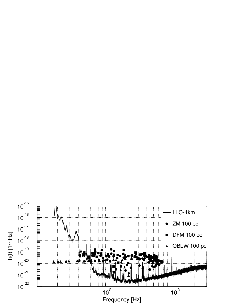
Figure 13: Signal strength $h_{\mathrm{rss}}$ at the detectors versus central frequency for the 176 supernovae waveforms from the three models described in references Zwerger and Müller (1997); Dimmelmeier et al. (2001); Ott et al. (2004): the hydrodynamical model of ref. Zwerger and Müller (1997), labeled “ZM”, the relativistic effects considered in ref. Dimmelmeier et al. (2001) and labeled “DFM”, and finally the hydrodynamical model employing realistic nuclear equation of state of ref. Ott et al. (2004), labeled “OBLW”. In all cases, the supernova events are positioned in optimal orientation and polarization at 100 pc from the detectors. The strain sensitivity of the L1 detector during the S2 run is shown for comparison.

For the case of binary black hole mergers, we have considered systems of black hole mass in the range of 10-90 $M_{\odot}$. The characteristic frequency of the resulting waveform is inversely proportional to the mass of the system and thus five different masses of 10, 30, 50, 70 and 90 $M_{\odot}$ were chosen in order to span the nominal frequency band of this search, i.e., the 100–1100 Hz band. Moreover, the waveforms of these systems Baker et al. (2002, 2004); ast come with two polarizations and they thus offered a check of the robustness of the waveform consistency test, the $r$-statistic, against complex morphologies. The efficiency is calculated over the whole sky considering the two polarization waveforms and a fixed inclination angle. The best performing mass system corresponds to 50 $M_{\odot}$: the characteristic frequency of this system corresponds to the best operating point of the LIGO instruments, i.e., close to 250 Hz. On the contrary, the two worst performing mass systems reflect frequencies at the two ends of the LIGO instrument’s sensitivities relevant to this search, i.e., 100 Hz and 1100 Hz. As with the supernova waveforms, the black-hole simulations provide us with order-of-magnitude estimates of the distance to which our detectors were sensitive to such astrophysical systems during the S2 run. For the Lazarus black-hole mergers our $h_{\mathrm{rss}}$ amplitudes of a few times $10^{-20}$ Hz^-1/2 correspond to distances of order 1 Mpc.

All four waveform families we have considered for our simulations, either ad hoc or astrophysically motivated, have frequency content that ranges over the entire band of our search. Within each of these families, signal strengths in order to reach fixed efficiency (e.g., 50%) range over approximately an order of magnitude; this is primarily a manifestation of the different frequency content of each waveform and the fact that the LIGO detectors’ frequency response is not flat (and varies by an order of magnitude or more over the 100–1100 Hz band, as shown in Fig. 1). We are in the process of augmenting the waveform library to be considered in future LIGO burst searches. This will give us further opportunities to test the robustness of our methods and the use of $h_{\mathrm{rss}}$ as a measure of the signal strength relevant to burst detection in LIGO.

X Summary and Discussion

We have presented a search for gravitational wave bursts using the data the three LIGO detectors collected during their second science run. Transients with sufficient energy in LIGO’s most sensitive band during the S2 run, 100–1100 Hz, were searched for. A search for gravitational wave bursts with frequency content above the 1100 Hz range is being pursued in coincidence with the TAMA Takahashi et al. (2004) detector and will be described in a separate publication ref (c). Our analysis yielded a single candidate event which was subsequently determined to be terrestrial in origin and was vetoed retroactively. Incorporating this into a frequentist statistical approach, we set an upper limit on the rate of strong gravitational wave bursts of $0.26$ events per day at the 90% confidence level. This rate limit is a factor of 6 below our previously published value Abbott et al. (2004c), due primarily to the longer duration of the S2 run and to better data quality.

The efficiency of this search was measured using various waveform morphologies. Besides the families of ad hoc waveforms we introduced in our previous search, we also measured the efficiency of our search to astrophysically motivated waveforms resulting from numerical simulations of the core collapse supernovae and binary black hole mergers. For most of the waveforms considered, the values of $h_{\mathrm{rss}}$ at 50% efficiency lie in the $10^{-20}-10^{-19}$ Hz^-1/2 range. The sensitivity attained by this search represents an improvement with respect to S1 by a factor of 17 or more for waveforms studied in both searches. This difference is frequency dependent and mainly reflects the instruments’ noise floor improvement by a factor of $\sim$10. The rest is attributed to improvements of the search algorithm and the use of the waveform consistency test ($r$-statistic), allowing a lower effective threshold on signal amplitude. The interpreted results of this search include the rate versus strength exclusion curves on a per waveform morphology basis. The improvements on the rate and signal strength sensitivity are both reflected in significantly more stringent regions now allowed in these rate versus strength plots.

X.1 Comparison with previous searches

In our S1 paper, we made a comparison with results from searches with broad-band interferometric detectors described in Nicholson et al. (1996); Forward (1978). The upper limit set by these detectors is at the level of 0.94 events per day and with a signal strength sensitivity of $h_{\mathrm{rss}}=5.9\times 10^{-18}$ Hz^-1/2, both of which are now surpassed by our S2 search. In our S1 paper we also compared with the results of the IGEC search for gravitational wave bursts Astone et al. (2003). LIGO’s broad band response allowed us to set better limits on bursts whose power was mainly at frequencies away from the bars’ resonances. At or near the bars’ resonant frequencies, however, the IGEC search benefited from a much longer observing time and somewhat better sensitivity at those frequencies, and thus was able to set rate limits far below what we were able to do in LIGO. With improved sensitivity in S2, it is interesting to again compare LIGO’s performance at a frequency near the bars’ resonance. In order to perform this comparison in our published S1 work Abbott et al. (2004c) we chose the sine-Gaussian simulations at 849 Hz frequency and with Q=8.9. Although this waveform morphology has significant signal power in the narrow frequency band (895–930 Hz) of sensitivity for most of the IGEC detectors, it actually fails to maintain an approximately flat Fourier spectrum over the broader range (694–930 Hz) needed in order to encompass all of them. For this reason, in order to perform the same comparison in S2 we have used the Gaussian of $\tau$=0.1 ms signal morphology which was the closest waveform with a flat spectrum in the 694–930 Hz range that we included in our S2 simulations.

The IGEC analysis Astone et al. (2003) set an upper limit of $\sim 4\times 10^{-3}$ events/day at the 95% confidence level on the rate of gravitational wave bursts. The limit was derived assuming optimal source direction and polarization and was also given as a function of the burst Fourier amplitude in a rate versus strength exclusion curve similar to LIGO’s. Using LIGO’s S2 Gaussian of $\tau$=0.1 ms simulations, the WaveBurst ETG efficiency for sources with random linear polarizations is 50% at a strength of $4.3\times 10^{-20}$ Hz^-1/2 (see Table 4). For the same sources all with optimal polarizations, the 50% efficiency point improves by roughly a factor of 3, to $1.6\times 10^{-20}$ Hz^-1/2. Thus the optimally oriented rate versus strength curve looks similar to Fig. 12, but shifted to the left. Substituting the 95% confidence level (CL) event limit of $0.33$ for the 90% CL event limit of $0.26$ shifts the curve up. Lastly, the IGEC excluded region from Fig. 13 of Astone et al. (2003) can be translated from bars’ natural units (Hz^-1) to units of $h_{\mathrm{rss}}$ (Hz^-1/2). Given the Fourier transform h(f) for a Gaussian waveform h(t),

$$h(t)=h_{\mathrm{rss}}\left(\frac{2}{\pi\tau^{2}}\right)^{1/4}\exp{(-t^{2}/\tau^{2})}$$ (16)

$$h(f)=h_{\mathrm{rss}}\left(2\pi\tau^{2}\right)^{1/4}\exp{(-\pi^{2}\tau^{2}f^{2})},$$ (17)

we convert the IGEC values of spectral amplitude h(f) into $h_{\mathrm{rss}}$ for a Gaussian of $\tau$=0.1 ms signal morphology (the conversion is a function of the assumed frequency of the IGEC result and may vary by a few percent over the 694–930 Hz range.) The resulting comparison can be seen in Fig. 14.

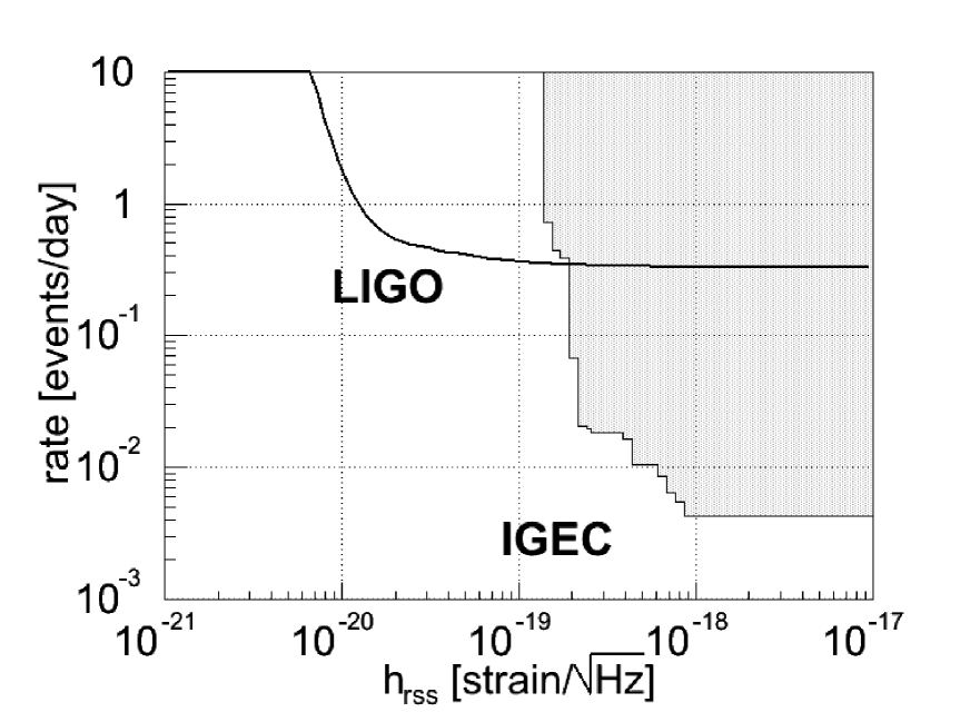
Figure 14: Rate versus $h_{\mathrm{rss}}$ exclusion curves at the 95% confidence level for optimally oriented Gaussians of $\tau$=0.1 ms. The solid curve displays the 95% confidence level measurement obtained by LIGO with this search. The IGEC exclusion region is shown shaded and it is adapted from Fig. 13 of Astone et al. (2003). If the comparison were performed using Q=8.9, 849 Hz sine-Gaussians, the LIGO and IGEC curves would move to smaller amplitudes by factors of 1.1 and $\sim$3, respectively.

With LIGO and S2 we are able to stretch the excluded region substantially to the left (i.e., to weaker signals) of the boundary of the excluded region in the rate versus strength curve of Fig. 13 in Astone et al. (2003). However, although S2’s increased observing time allows a lower rate limit than could be set in S1, it is still the case that the IGEC longer duration search allows substantially better rate limits to be set, for signals strong enough for its detectors to have seen them.

Furthermore, we are interested in a comparison with the results reported from the analysis of the EXPLORER and NAUTILUS 2001 data. In their 2002 paper Astone et al. (2002b) the Rome group that analyzes the data of and operates these two resonant mass detectors reported a slight excess of events seen in sidereal hours between 3 and 5. The events seen in concidence by the two detectors are of an average temperature of approximately 120mK which according to the authors corresponds to an optimally oriented gravitational wave burst Fourier amplitude of $2.7\times 10^{-21}$Hz^-1 (equation 4 from ref. Astone et al. (2002b)). The rate of such events is of order 200 events/year (or 0.55 events/day) Astone et al. (2002b); Coccia et al. (2004). Given the amplitude of the observed events by the resonant mass detectors, the corresponding $h_{\mathrm{rss}}$ of the hypothetical events in our LIGO instruments will generally depend on the signal morphology. As with our aforementioned IGEC analysis, we considered the case of a Gaussian of $\tau$=0.1 ms, for which the Fourier amplitude of the observed events at the detectors’ average resonance frequency implies an $h_{\mathrm{rss}}$ of $1.9\times 10^{-19}$ Hz^-1/2. Keeping in mind that the suggested $h_{\mathrm{rss}}$ values refer to optimal orientation, we can see from Fig. 14 that for this event strength the LIGO S2 search set an upper bound to their flux at roughly $0.4$ events per day at the 95% CL. It should be noted, though, that depending on the assumptions of signal waveform (for example a single cycle of a 914 Hz sinusoid or a narrow-band sine-Gaussian signal centered on the same frequency) or considering the range of event strengths recorded by EXPLORER and NAUTILUS (rather than their average value only) the corresponding $h_{\mathrm{rss}}$ at the LIGO detectors may come nearer to the threshold of our sensitivity and thus make our rate limits poorer. The signal strength and rate of the 2001 Rome results come with enough uncertainties that given the LIGO S2 sensitivity and exposure we cannot make a definitive comparison. The significant improvements in sensitivity and longer observation times that we expect in new LIGO searches in the near future will enable us to move in this direction.

X.2 Discussion and future directions

The search for gravitational wave bursts in LIGO’s S2 run has seen significant improvements introduced in the search methodology and interpretation with respect to S1. This included the introduction of the waveform consistency cut and the use of astrophysically motivated waveforms as part of the search interpretation. Additional improvements are currently under way. We expect them to bring stronger suppression of the background via the use of a burst amplitude consistency test between the LIGO detectors as well as new ways of performing our event analysis within the context of a distributional analysis of their strength. Moreover, we plan to make use of data taking periods corresponding to the double coincidence of the instruments that are not part of the triple coincidence dataset. We will continue investigating the optimization of search algorithms for specific types of waveforms and adding stronger astrophysical context in our search by invoking source population models or targeting plausible point sources. Among the lessons learned in the S2 search has been the importance of the follow-up investigations dictated by coincident triggers revealed by the pipeline. As expected, with the detector performance nearing design sensitivity, potential couplings from the environment and the instrument itself will become apparent and will need to be identified and vetoed out. Our on-going work for vetoes will become more prominent together with the need to define rigorous criteria and procedures for following up on such events. LIGO’s subsequent runs have already collected data of comparable duration and improved sensitivity with respect to S2 and they will present the next milestone of the search for bursts where a good number of these improvements will be exercised.

The software used in this analysis is available in the LIGO Scientific Collaboration’s CVS archives at http://www.lsc-group.phys.uwm.edu/cgi-bin/ cvs/viewcvs.cgi/?cvsroot=lscsoft under the S2_072704 tag for WaveBurst in LAL and LALWRAPPER and rStat-1-2 tag for $r$-statistic in MATAPPS.