Discrete space-time

Abstract

We review recent efforts to construct gravitational theories on discrete space-times, usually referred to as the “consistent discretization” approach. The resulting theories are free of constraints at the canonical level and therefore allow to tackle many problems that cannot be currently addressed in continuum quantum gravity. In particular the theories imply a natural method for resolving the big bang (and other types) of singularities and predict a fundamental mechanism for decoherence of quantum states that might be relevant to the black hole information paradox. At a classical level, the theories may provide an attractive new path for the exploration of issues in numerical relativity. Finally, the theories can make direct contact with several kinematical results of continuum loop quantum gravity. We review in broad terms several of these results and present in detail as an illustration the classical treatment with this technique of the simple yet conceptually challenging model of two oscillators with constant energy sum.

I Introduction

The idea that space-time might be discrete has arisen at various levels in gravitational physics. On one hand, some approaches hypothesize that at a fundamental level a discrete structure underlies space-time. Other approaches start with a continuum theory but upon quantization discrete structures associated with space-time emerge. Finally, discretizations are widely used in physics, and in gravity in particular, as a calculational tool at two levels: a) at the time of numerically computing predictions of the theory (classical and quantum mechanically) and b) as a regularization tool for quantum calculations.

Whatever the point of view that may lead to the consideration of a discrete space-time, the formulation of gravitational theories on such structures presents significant challenges. At the most immediate level, the presence of discrete structures can conflict with diffeomorphism invariance, a desirable property of gravitational theories. This manifests itself in various ways. For instance, if one simply proceeds to discretize the equations of motion of general relativity, as is common in numerical relativity applications, one finds that the resulting equations are inconsistent: the evolution equations do not preserve the constraints, as they do in the continuum. In another example, if one considers the discretization of the constraints of canonical quantum gravity, the resulting discrete constraints fail to close an algebra, which can be understood as another manifestation of the inconsistency faced in numerical relativity.

A new viewpoint has recently emerged towards the treatment of theories on discrete space-times. At the most basic level, the viewpoint advocates discretizing the action of the theory and working out the resulting equations of motion rather than discretizing the equations of motion directly. The resulting equations of motion stemming from the discrete action are generically guaranteed to be consistent. So immediately the problem of consistency is solved. This has led to the approach being called the “consistent discretization” approach. This approach has been pursued in the past in numerical approaches to unconstrained theories and is known as “variational integrators” (see Marsd for a review) and it appears to have several desirable properties. Constrained systems have only been considered if they are holonomic (i.e. they only depend on the configuration variables), although see mclc for some recent results for anholonomic constraints.

In spite of these positive prospects, the resulting theories have features that at first sight may appear undesirable. For instance, quantities that in the usual continuum treatment are Lagrange multipliers of first class constrained systems (and therefore freely specifiable), become determined by the equations of motion. The equations that determine the Lagrange multipliers in general may have undesirable complex solutions.

On the other hand, the approach has potentially very attractive features: equations that in the continuum are constraints among the dynamical variables become evolution equations that are automatically solved by the scheme. Having no constraints in the theory profoundly simplifies things at the time of quantization. The conceptually hard problems of canonical quantum gravity are almost entirely sidestepped by this approach. For instance, one can introduce a relational description in the theory and therefore solve the “problem of time” that created so much trouble in canonical quantum gravity. The resulting relational description naturally implies a loss of unitarity that may have implications for the black hole information puzzle. The discrete theories also have a tendency to avoid singularities, since the latter usually do not fall on the computational grid. At a quantum level this implies that singularities have zero probability. This provides a singularity avoidance mechanism that is distinct from the one usually advocated in loop quantum cosmology. From the point of view of numerical relativity, the resulting evolution schemes preserve the constraints of the continuum theory to a great degree of accuracy, at least for solutions that approximate the continuum limit. This is different from usual “free evolution” schemes which can converge to continuum solutions that violate the constraints. As we will see, we are still somewhat away from being able to advocate that the resulting schemes can be competitive in numerical relativity. But given that enforcing the constraints has been identified by some researchers as the main obstacle to numerical relativity, the proposed schemes deserve some consideration.

An aspect of presupposing a discrete structure for space-time that may also appear undesirable is that in loop quantum gravity the discrete structures only emerge after quantization. The initial formulation of the theory is in the continuum. Therefore there is the risk that the new viewpoint may not be able to make contact with the many attractive kinematical results of loop quantum gravity. We will see that a connection is in fact possible, and it retains the attractive aspects of both approaches.

In this paper we would like to review the “consistent discretization” approach to gravitational theories. In section II we will outline the basics of the strategy. In section III we concretely apply the method to a simple yet important model problem so the reader can get a flavor of what to expect from the method classically. In section IV we discuss cosmological models and in section V the introduction of a relational time and the black hole information puzzle. In section VI we discuss connections with continuum loop quantum gravity. We end with a discussion.

II Consistent discretizations

We start by considering a continuum theory representing a mechanical system. Although our ultimate interest is in field theories, the latter become mechanical systems when discretized. Its Lagrangian will be denoted by ${\hat{L}(q^{a},\dot{q}^{a})}$, $a=1\ldots M$. This setting is general enough to accommodate, for instance, totally constrained systems. In such case $\dot{q}$ will be the derivative of the canonical variables with respect to the evolution parameter. It is also general enough to include the systems that result from formulating on a discrete space-time lattice a continuum field theory.

We discretize the evolution parameter in intervals (possibly varying upon evolution) $t_{n+1}-t_{n}=\epsilon_{n}$ and we label the generalized coordinates evaluated at $t_{n}$ as $q_{n}$. We define the discretized Lagrangian as

$$L(n,n+1)\equiv L(q^{a}_{n},q^{a}_{n+1})\equiv\epsilon_{n}{\hat{L}}(q^{a},\dot{q}^{a})$$ (1)

where

$$q^{a}=q^{a}_{n}\quad\hbox{and}\quad\dot{q}^{a}\equiv{{q^{a}_{n+1}-q^{a}_{n}}\over\epsilon_{n}}.$$ (2)

Of course, one could have chosen to discretize things in a different fashion, for instance using a different approximation for the derivative, or by choosing to write the continuum Lagrangian in terms of different variables. The resulting discrete theories generically will be different and will approximate the continuum theory in different ways. However, given a discrete theory, the treatment we outline in this paper is unique.

The action can then be written as

$$S=\sum_{n=0}^{N}L(n,n+1).$$ (3)

It should be noted that in previous treatments DiGaPu ; GaPu we have written the Lagrangian in first order form, i.e. $L=\int dt\left(p\dot{q}-H(p,q)\right)$. It should be emphasized that this is contained as a particular case in the treatment we are presenting in this paper. In this case one takes both $q$ and $p$ to be configuration variables, and one is faced with a Lagrangian that involves $q_{n},p_{n}$ and $q_{n+1}$ as variables, being independent of $p_{n+1}$.

If the continuum theory is invariant under reparameterizations of the evolution parameter, one can show that the information about the intervals $\epsilon_{n}$ may be absorbed in the Lagrange multipliers. In the case of standard mechanical systems it is simpler to use an invariant interval $\epsilon_{n}=\epsilon$.

The Lagrange equations of motion are obtained by requiring the action to be stationary under variations of the configuration variables $q^{a}$ fixed at the endpoints of the evolution interval $n=0,n=N+1$,

$${\partial L(n,n+1)\over\partial q^{a}_{n}}+{\partial L(n-1,n)\over\partial q^{a}_{n}}=0.$$ (4)

We introduce the following definition of the canonically conjugate momenta of the configuration variables,

$$p^{a}_{n+1} \equiv {\partial L(n,n+1)\over\partial q^{a}_{n+1}}$$ (5)

$$p^{a}_{n} \equiv {\partial L(n-1,n)\over\partial q^{a}_{n}}=-{\partial L(n,n+1)\over\partial q^{a}_{n}}$$ (6)

Where we have used Eq. (4). The equations (5) and (6) define a canonical transformation for the variables $q_{n},p_{n}$ to $q_{n+1},p_{n+1}$ with a the type 1 generating function $F_{1}=-L(q^{a}_{n},q^{a}_{n+1})$. Notice that the evolution scheme is implicit, one can use the bottom equation (since we are in the non-singular case) to give an expression for $q_{n+1}$ in terms of $q_{n},p_{n}$, which in turn can be substituted in the top equation to get an equation for $p_{n+1}$ purely in terms of $q_{n},p_{n}$.

It should be noted that there are several other possible choices, when going from the set of equations (5,6) to an explicit evolution scheme (see jmp for further details.)

The canonical transformation we introduced becomes singular as an evolution scheme if $\displaystyle\left|{\partial^{2}L(n,n+1)\over\partial q^{a}_{n+1}\partial q^{b}_{n}}\right|$ vanishes. If the rank of the matrix of second partial derivatives is $K$ the system will have $2(M-K)$ constraints of the form,

$$\Phi_{A}(q^{a}_{n},p^{a}_{n}) = 0$$ (7)

$$\Psi_{A}(q^{a}_{n+1},p^{a}_{n+1}) = 0.$$ (8)

And these constraints need to be enforced during evolution, which may lead to new constraints. We refer the reader for the detailed Dirac analysis to jmp .

To clarify ideas, let us consider an example. The model consists of a parameterized free particle in a two dimensional space-time under the influence of a linear potential. The discrete Lagrangian is given by,

$$L_{n}\equiv L(q_{n}^{a},\pi_{n}^{a},N_{n},q_{n+1}^{a},\pi_{n+1}^{a},N_{n+1})=\pi_{n}^{a}(q_{n+1}^{a}-q^{a}_{n})-N_{n}[\pi_{n}^{0}+\frac{1}{2}(\pi_{n}^{1})^{2}+\alpha q_{n}^{1}].$$ (9)

We have chosen a first order formulation for the particle. However, this Lagrangian is of the type we considered in this paper, one simply needs to consider all variables, $q^{a},\pi^{a},N$ as configuration variables. The system is clearly singular since the $\pi^{\prime}s$ and $N$ only appear at level $n$ (or in the continuum Lagrangian, their time derivatives are absent). When considered as a Type I generating function, the above Lagrangian leads to the equations

$$p^{a}_{\pi,\,n+1} = \frac{\partial L_{n}}{\partial\pi^{a}_{n+1}}=0,$$ (10)

$$p^{a}_{q,\,n+1} = \frac{\partial L_{n}}{\partial q^{a}_{n+1}}=\pi_{n}^{a},$$ (11)

$$p_{N,\,n+1} = \frac{\partial L_{n}}{\partial N_{n+1}}=0,$$ (12)

and

$$p^{a}_{\pi,\,n} = -\frac{\partial L_{n}}{\partial\pi^{a}_{n}}=-(q_{n+1}^{a}-q_{n}^{a})+\pi_{n}^{1}N_{n}\delta^{a}_{1}+N_{n}\delta^{a}_{0},$$ (13)

$$p^{a}_{q,\,n} = -\frac{\partial L_{n}}{\partial q^{a}_{n}}=\pi_{n}^{a}+\delta^{a}_{1}\alpha N_{n},$$ (14)

$$p_{N,\,n} = -\frac{\partial L_{n}}{\partial N_{n}}=\pi_{n}^{0}+\frac{1}{2}(\pi_{n}^{1})^{2}+\alpha q_{n}^{1}.$$ (15)

The constraints (10,12,14,15) can be imposed strongly to eliminate the $\pi$’s and the $N$’s and obtain an explicit evolution scheme for the $q$’s and the $p_{q}$’s,

$$q^{0}_{n} = q^{0}_{n+1}-\frac{C_{n+1}}{\alpha p^{1}_{q,\,n+1}},$$ (16)

$$q^{1}_{n} = q^{1}_{n+1}-\frac{C_{n+1}}{\alpha},$$ (17)

$$p^{0}_{q,\,n} = p^{0}_{q,\,n+1},$$ (18)

$$p^{1}_{q,\,n} = p^{1}_{q,\,n+1}+\frac{C_{n+1}}{p^{1}_{q,\,n+1}},$$ (19)

and the Lagrange multipliers get determined to be,

$$N_{n}=\frac{C_{n+1}}{\alpha p^{1}_{q,\,n+1}},$$ (20)

where $C_{n+1}=p^{0}_{q,\,n+1}+(p^{1}_{q,\,n+1})^{2}/2+\alpha q^{1}_{n+1}$. The evolution scheme runs backwards, one can construct a scheme that runs forward by solving for $N$ and $\pi$ at instant $n$ when imposing the constraints strongly. The two methods yield evolution schemes of different functional form since one propagates “forward” in time and the other “backward”. The inequivalence in the functional form stems from the fact that the discretization of the time derivatives chosen in the Lagrangian is not centered. It should be emphasized that if one starts from given initial data and propagates forwards with the first system of equations and then backwards using the second, one will return to the same initial data.

So we see in the example how the mechanism works. It yields evolution equations that usually are implicit as evolution schemes. The equations are consistent. The Lagrange multipliers get determined by the scheme and there are no constraints left on the canonical variables. The evolution is implemented by a (non-singular) canonical transformation. The number of degrees of freedom is larger than those in the continuum. There will exist different sets of initial data that lead to different solutions for the discrete theory but nevertheless will just correspond to different discrete approximations and parameterizations of a single evolution of the continuum theory.

III The Rovelli model

To analyze the method in a simple —yet challenging— model we consider the model analyzed by Rovelli Rovelli in the context of the problem of time in canonical quantum gravity: two harmonic oscillators with constant energy sum. The intention of this section is to illustrate how the method works and some of the expectations one can hold when applying the method to more complex situations. The model itself can obviously be treated with more straightforward discretization techniques given its simplicity. The fact that the method works well for the model should not be construed as proof that it will be successful in other numerical applications. Current efforts suggest that the technique is successfully applicable to Gowdy cosmologies.

The model has canonical coordinates $q^{1},q^{2},p^{1},p^{2}$ with the standard Poisson brackets and a constraint given by,

$$C=\frac{1}{2}\left((p^{1})^{2}+(p^{2})^{2}+(q^{1})^{2}+(q^{2})^{2}\right)-M=0,$$ (21)

with $M$ a constant. No Hamiltonian system can correspond to this dynamical system since the presymplectic space is compact and therefore cannot contain any $S\times R$ structure. Nevertheless, we will see that the consistent discretization approach does yield sensible results. This helps dispel certain myths about the consistent discretization scheme. Since it determines Lagrange multipliers a lot of people tend to associate the scheme as some sort of “gauge fixing”. For this model however, a gauge fixing solution would be unsatisfactory, since it would only cover a portion of phase space. We will see this is not the case in the consistent discretization scheme. We will also see that the evolution scheme is useful numerically in practice.

We start by writing a discrete Lagrangian for the model,

$$L(n,n+1)=p^{1}_{n}\left(q^{1}_{n+1}-q^{1}_{n}\right)+p^{2}_{n}\left(q^{2}_{n+1}-q^{2}_{n}\right)-\frac{N_{n}}{2}\left((p^{1}_{n})^{2}+(p^{2}_{n})^{2}+(q^{1}_{n})^{2}+(q^{2}_{n})^{2}-2M\right),$$ (22)

and working out the canonical momenta for all the variables, i.e., $P_{q}^{1},P_{q}^{2},P_{p}^{1},P_{p}^{2}$. One then eliminates the $p^{1,2}$ and the $P_{p}^{1,2}$ and is left with evolution equations for the canonical pairs,

$$q^{1}_{n+1} = q^{1}_{n}+N_{n}\left(P^{1}_{q,n}-2q^{1}_{n}\right)$$ (23)

$$q^{2}_{n+1} = q^{2}_{n}+N_{n}\left(P^{2}_{q,n}-2q^{2}_{n}\right)$$ (24)

$$P^{1}_{q,n+1} = P^{1}_{q,n}-N_{n}q^{1}_{n}$$ (25)

$$P^{2}_{q,n+1} = P^{2}_{q,n}-N_{n}q^{2}_{n}.$$ (26)

The Lagrange multiplier gets determined by the solution(s) of a quadratic equation,

$$\left((q^{1}_{n})^{2}+(q^{2}_{n})^{2}\right)(N_{n})^{2}-2\left(P^{1}_{q,n}q^{1}_{n}+P^{2}_{q,n}q^{2}_{n}\right)N_{n}+\left(P^{1}_{q,n}\right)^{2}+\left(P^{2}_{q,n}\right)^{2}+\left(q^{1}_{n}\right)^{2}+\left(q^{2}_{n}\right)^{2}-2M=0.$$ (27)

We would like to use this evolution scheme to follow numerically the trajectory of the system. For this, we need to give initial data. Notice that if one gives initial data that satisfy the constraint identically at level $n$, the quadratic equation for the lapse has a vanishing independent term and therefore the solution is that the lapse $N$ vanishes (the nonvanishing root will be large and far away from the continuum generically). To construct initial data one therefore considers a set for which the constraint vanishes and introduces a small perturbation on one (or more) of the variables. Then one will have evolution. Notice that one can make the perturbation as small as desired. The smaller the perturbation, the smaller the lapse and the closer the solution will be to the continuum.

For concreteness, we choose the following initial values for the variables, $M=2$,

$$q^{1}_{0} = 0,$$ (28)

$$q^{2}_{0} = (\sqrt{3}-\Delta)\sin({\pi\over 4}),$$ (29)

$$P^{1}_{q,0} = 1,$$ (30)

$$P^{1}_{q,0} = (\sqrt{3}-\Delta)\cos({\pi\over 4}),$$ (31)

We choose the parameter $\Delta$ to be the perturbation, i.e., $\Delta=0$ corresponds to an exact solution of the constraint, for which the observable $A=1/2$ (see below for its definition). The evolution scheme can easily be implemented using a computer algebra program like Maple or Mathematica.

Before we show results of the evolution, we need to discuss in some detail how the method determines the lapse. As we mentioned, it is obtained by solving the quadratic equation (27). This implies that generically there will be two possible solutions and in some situations they could be negative or complex. One can choose any of the two solutions at each point during the evolution. It is natural numerically to choose one “branch” of the solution and keep with it. However, if one encounters that the roots become complex, we have observed that it is possible to backtrack to he previous point in the iteration, choose the alternate root to the one that had been used up to that point and continue with the evolution. Similar procedure could be followed when the lapse becomes negative. It should be noted that negative lapses are not a problem per se, it is just that the evolution will be retraced backwards. We have not attempted to correct such retracings, i.e. in the evolutions shown we have only “switched branches” whenever the lapse becomes complex. This occurs when the discriminant in the quadratic equation (27) vanishes.

Figure (1) shows the evolution of $q_{1}$ as a function of $n$. The figure looks choppy since the “rate of advance” (magnitude of the lapse) varies during the evolution.

Figure 1: The evolution of one of the variables of the oscillator model as a function of the discretization parameter $n$. The irregular nature of the curve is due to the fact that the lapse is a dynamical variable and therefore the rate of advance changes during evolution. The sharp feature around $n=250$ is due to the fact that the lapse becomes negative and the evolution runs backwards for a while, until about $n=310$.

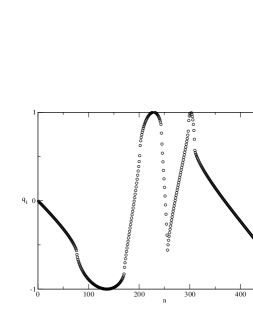
Figure (1) also exhibits that in a reparameterization invariant theory like this one it is not too useful to plot parameterization dependent quantities. One would have to exhibit relational quantities that are true observables of the theory to obtain physically relevant information. In this particular model, Rovelli has given an explicit expression for a relational (“evolving”) observable

$$q^{2}(q^{1})=\sqrt{M/A-1}\left[q^{1}\cos\phi\pm\sqrt{2A-(q^{1})^{2}}\sin\phi\right],$$ (32)

where $A$ and $\phi$ are constants of the motion (“perennials”), whose expression in terms of the coordinates is,

$$4A = 2M+(p^{1})^{2}-(p^{2})^{2}+(q^{1})^{2}-(q^{2})^{2},\tan\phi={p^{1}q^{2}-p^{2}q^{1}\over p^{1}p^{2}+q^{2}q^{1}}.$$ (33)

The relational observable gives an idea of the trajectory in configuration space in a manner that is invariant under reparameterizations. In figure (2) we show the error in the evaluation of the relational observable with respect to the exact expression of the continuum in our model.

Figure 2: The error in the evaluation of the relational observable in the discretized evolution, compared with respect to the exact continuum expression. We show the absolute error, but since the quantities are of order one it can also be understood as the relative error. The peaks in the error are due to the functional form of the observable involving the square root of $2A-q_{1}^{2}$. This vanishes when $q_{1}=\pm 1$ (see previous plot) and this magnifies the error in the observable.

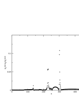
This model has two independent “perennials” that can be used to construct relational observables like the one we just discussed. The first one of these perennials happens to be an exact conserved quantity of the discretized theory. The relation between perennials in the continuum and conserved quantities of the discrete theory was further discussed in cosmo . The perennial in question is,

$$O_{1}=p^{1}q^{2}-p^{2}q^{1}.$$ (34)

Another perennial is given by

$$O_{2}=(p^{1})^{2}-(p^{2})^{2}+(q^{1})^{2}-(q^{2})^{2}.$$ (35)

This quantity is not an exact conserved quantity of the discrete model, it is conserved approximately, as we can see in figure (3). We see that the discrete theory conserves the perennial quite well in relative error and even though in intermediate steps of the evolution the error grows, it decreases later.

Figure 3: The model has two “perennials”. One of them is an exact conserved quantity of the discrete theory, so we do not present a plot for it. The second perennial $(O_{2})$ is approximately conserved. The figure shows the relative error in its computation in the discrete theory. It is worthwhile noticing that, unlike what is usual in free evolution schemes, errors do not accumulate, they may grow for a while but later they might diminish.

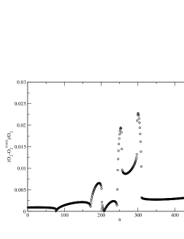
In figure (4) we depict the absolute value of the constraint of the continuum theory as a function of discrete time $n$. It is interesting to observe that in the discrete theory the variables approximate the ones of the continuum with an error that is proportional to the value of the constraint. Therefore the value of the constraint can be taken as an indicator of how accurately one is mirroring the continuum theory. It is a nice feature to have such an error indicator that is independent of the knowledge of the exact solution. This is clearly exhibited by contrasting (4) with (3) and seeing how the value of the constraint mirrors the error in the perennial. It should be noted that the proportionality factor between the value of the constraint and the error is a function of the dynamical variables and therefore the value of the constraint should only be taken as an indicator, not an exact measure of the error. However, it is a good indicator when one carries out convergence studies, since there the dynamical variables do not change in value significantly from one resolution to the next and the constraint diminishes as one converges to the continuum.

Figure 4: Absolute value of the constraint of the continuum theory, evaluated in the discrete theory. The plot shows that the constraint of the continuum theory does not increase in the discrete theory as a function of evolution (a major desired goal in numerical relativity). The value of the constraint is also a measure of the error in the quantities of the discrete theory with respect to those of the continuum one (compare with the error in the observable in figure 3, for example) that can be used to independently assess the accuracy of the theory in convergence studies.

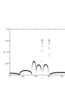
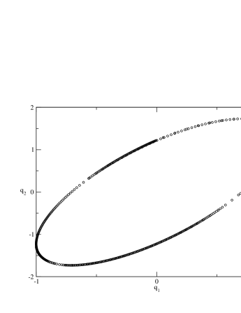
Figure (5) shows the trajectory in configuration space. As we see, the complete trajectory is covered by the discretized approach. This is important since many people tend to perceive the consistent discretization approach as “some sort of gauge fixing”. This belief stems from the fact that when one gauge fixes a theory, the multipliers get determined. In spite of this superficial analogy, there are many things that are different from a gauge fixing. For instance, as we discussed before, the number of degrees of freedom changes. In addition to this, this example demonstrates another difference. If one indeed had gauge fixed this model, one would fail to cover the entire available configuration space, given its compact nature.

Figure 5: The orbit in configuration space. As it is readily seen, the consistent discrete approach covers the entire available configuration space. This clearly exhibits that the approach is not a “gauge fixing”. Gauge fixed approaches cannot cover the entire configuration space due to its compact nature. The dynamical changes in the value of the lapse can be seen implicitly through the density of points in the various regions of the trajectory. Also apparent is that the trajectory is traced on more than one occasion in various regions. Deviation from the continuum trajectory is not noticeable in the scales of the plot.

An issue of interest in any numerical method is the concept of convergence. Any reasonable numerical scheme should be such that one has control on the approximation of the exact solution. Figure (6) shows the convergence in the error of the estimation of the observable $O_{2}$. We see that one has convergence in the traditional sense, i.e. making the discretization step smaller lowers the errors. However, one notes differences with the usual type of convergence in the sense that here we have that it is not uniform as a function of the evolution time. One notes, for example, that at isolated points some of the coarser runs have very low errors. To understand this one needs to recall that in our approach discrete expressions differ from the continuum ones as,

$$O=O_{\rm continuum}+f(p,q)C$$ (36)

with $C$ the constraints. It could happen that at a particular point in a coarse evolution the constraint chances to take a value very close to zero. Slightly finer resolution runs may not land on top of that particular point and therefore will apparently have larger errors in the region. Eventually, if one increases the resolution enough, one will be able to achieve better accuracy than with the coarser run.

Figure 6: Convergence of the method with increasing resolution. We display the relative error in one of the perennials of the theory as a function of $n$. The two runs with the coarser resolutions are shown with one point out of every ten displayed. The finer run is shown with one point displayed out of every thirty. The range of $n$ displayed corresponds to a full trajectory along the ellipse in configuration space. So the improvement in accuracy is throughout the entire evolution with different levels of improvement at different points. See the text as to why we fine tune the evolution steps for the various runs in the convergence study.

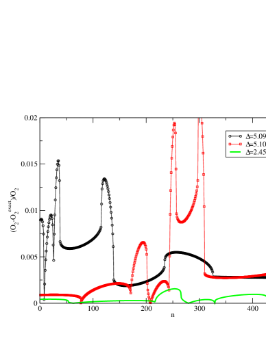
The reader may ponder why the parameter we have chosen to characterize the discretization is listed with several digits of precision in the convergence runs. The reason is the following: our algorithm exhibits some sensitivity on the parameter in the following sense. If one chooses slightly different values of $\Delta$, the way in which the scheme will usually cover the phase space will be different. For instance, one choice may cover the configuration space ellipse in one continuous sweep, another close choice may reverse course several times before covering the ellipse. From a physical point of view this is no problem, but from the point of view of comparing runs as a function of $n$ one wishes to compare runs that behave in the same way. Therefore when one “halves the stepsize” one may need to fine tune by trial an error to make sure one is comparing evolutions that behave similarly in terms of the (unphysical) parameter $n$.

IV Applications in quantum cosmology

To try to seek an application more connected with gravitational physics, yet simple enough that we can solve things analytically, let us consider a cosmological model. The model in question will be a Friedmann model with a cosmological constant and a scalar field. To make the solution of the model analytically tractable we will consider a very massive scalar field (i.e. we will ignore the kinetic term of the field in the action). We have actually solved this and other models without this approximation numerically and obtained results that are conceptually similar to the ones we present here.

The Lagrangian for the model, written in terms of Ashtekar’s new variables (there is no impediment in treating the model with traditional variables if one wishes) is,

$$L=E\dot{A}+\pi\dot{\phi}-NE^{2}(-A^{2}+(\Lambda+m^{2}\phi^{2})|E|)$$ (37)

where $\Lambda$ is the cosmological constant, $m$ is the mass of the scalar field $\phi$, $\pi$ is its canonically conjugate momentum and $N$ is the lapse with density weight minus one. Here $E$ and $A$ are the functions of time which are what remains of the triad and connection for the homogeneous case. The appearance of $|E|$ in the Lagrangian is due to the fact that the term cubic in $E$ is supposed to represent the spatial volume and therefore should be positive definite. In terms of the ordinary lapse $\alpha$ we have $\alpha=N|E|^{3/2}$. The equations of motion and the only remaining constraint (Hamiltonian) are

$$\dot{A} = N(\Lambda+m^{2}\phi^{2}){\rm sgn}(E)E^{2}$$ (38)

$$\dot{E} = 2NE^{2}A$$ (39)

$$\dot{\phi} = 0$$ (40)

$$\dot{\pi} = -2N|E|^{3}m^{2}\phi$$ (41)

$$A^{2} = (\Lambda+m^{2}\phi^{2})|E|$$ (42)

It immediately follows from the large mass approximation that $\phi={\rm constant}$. To solve for the rest of the variables, we need to distinguish four cases, depending on the signs of $E$ and $A$. Let us call $\epsilon={\rm sgn}(E)$ and $\chi={\rm sgn}(A)$. Then the solution (with the choice of lapse $\alpha=1$) is,

$$A = \chi\exp\left(\chi\epsilon t\sqrt{\Lambda+m^{2}\phi^{2}}\right)$$ (43)

$$E = \epsilon{\exp\left(2\chi\epsilon t\sqrt{\Lambda+m^{2}\phi^{2}}\right)\over{\Lambda+m^{2}\phi^{2}}}$$ (44)

There are four possibilities according to the signs $\epsilon,\chi$. If $\epsilon=\chi=1$ or $\epsilon=\chi=-1$ we have a universe that expands. If both have different signs, the universe contracts. This just reflects that the Lagrangian is invariant if one changes the sign of either $A$ or $E$ and the sign of time. It is also invariant if one changes simultaneously the sign of both $A$ and $E$.

Let us turn to the observables of the theory (quantities that have vanishing Poisson brackets with the constraint (42) and therefore are constants of the motion). The theory has four phase space degrees of freedom with one constraint, therefore there should be two independent observables. Immediately one can construct an observable $O_{1}=\phi$, since the latter is conserved due to the large mass approximation. To construct the second observable we write the equation for the trajectory,

$${d\pi\over dA}={-2Em^{2}\phi\over\Lambda+m^{2}\phi^{2}}=-{2A^{2}m^{2}\phi\over\left(\Lambda+m^{2}\phi^{2}\right)^{2}}{\rm sgn}E$$ (45)

where in the latter identity we have used the constraint. Integrating, we get the observable,

$$O_{2}=\pi+{2\over 3}{m^{2}\phi\over\left(\Lambda+m^{2}\phi^{2}\right)^{2}}A^{3}{\rm sgn}E$$ (46)

and using the constraint again we can rewrite it,

$$O_{2}=\pi+{2\over 3}{m^{2}\phi\over\Lambda+m^{2}\phi^{2}}AE.$$ (47)

Although the last two expressions are equivalent, we will see that upon discretization only one of them becomes an exact observable of the discrete theory.

We consider the evolution parameter to be a discrete variable. Then the Lagrangian becomes

$$L(n,n+1)=E_{n}(A_{n+1}-A_{n})+\pi_{n}(\phi_{n+1}-\phi_{n})-N_{n}E_{n}^{2}(-A^{2}_{n}+(\Lambda+m^{2}\phi^{2}_{n})|E_{n}|)$$ (48)

The discrete time evolution is generated by a canonical transformation of type 1 whose generating function is given by $-L$, viewed as a function of the configuration variables at instants $n$ and $n+1$. The canonical transformation defines the canonically conjugate momenta to all variables. The transformation is such that the symplectic structure so defined is preserved under evolution. The configuration variables will be $(A_{n},E_{n},\pi_{n},\phi_{n},N_{n})$ with canonical momenta $(P^{A}_{n},P^{E}_{n},P^{\phi}_{n},P^{\pi}_{n},P^{N}_{n})$ defined in the traditional fashion by functional differentiation of the action with respect to the canonical variables. We do not reproduce their explicit expression here for reasons of brevity, the reader can consult them in reference cosmo . The definitions of the momenta can be combined in such a way as to yield a simpler evolution system,

$$A_{n+1}-A_{n} = N_{n}(P^{A}_{n+1})^{2}_{n}(\Lambda+m^{2}\phi^{2}_{n}){\rm sgn}P^{A}_{n+1},$$ (49)

$$P^{A}_{n+1}-P^{A}_{n} = 2N_{n}A_{n}(P^{A}_{n+1})^{2}$$ (50)

$$\phi_{n+1}-\phi_{n} = 0$$ (51)

$$P^{\phi}_{n+1}-P^{\phi}_{n} = -2N_{n}(P^{A}_{n+1})^{2}m^{2}\phi_{n}|P^{A}_{n+1}|,$$ (52)

$$0 = -A^{2}_{n}+(\Lambda+m^{2}\phi^{2}_{n})|P^{A}_{n+1}|,$$ (53)

and the phase space is now spanned by $A_{n},P^{A}_{n},\phi_{n},P^{\phi}_{n}$.

From (50) we determine,

$$P^{A}_{n+1}={1+\xi\sqrt{1-8P^{A}_{n}A_{n}N_{n}}\over 4A_{n}N_{n}},$$ (54)

where $\xi=\pm 1$ and we will see the final solution is independent of $\xi$. Substituting in (53) and solving for the lapse we get,

$$N_{n}={\left[-P^{A}_{n}\left(\Lambda+m^{2}\phi_{n}^{2}\right)+A_{n}^{2}{\rm sgn}P^{A}_{n}\right]\left(\Lambda+m^{2}\phi_{n}^{2}\right)\over 2A_{n}^{5}}.$$ (55)

Let us summarize how the evolution scheme presented actually operates. Let us assume that some initial data $A^{(0)},P^{A}_{(0)}$, satisfying the constraints of the continuum theory, are to be evolved. The recipe will consist of assigning $A_{0}=A^{(0)}$ and $P^{A}_{1}=P^{A}_{(0)}$. Notice that this will automatically satisfy (53). In order for the scheme to be complete we need to specify $P^{A}_{0}$. This is a free parameter. Once it is specified, then the evolution equations will determine all the variables of the problem, including the lapse. Notice that if one chooses $P^{A}_{0}$ such that, together with the value of $A_{0}$ they satisfy the constraint, then the right hand side of the equation for the lapse (55) would vanish and no evolution takes place. It is clear that one can choose $P^{A}_{0}$ in such a way as to make the evolution step as small as desired.

The equation for the lapse (55) implies that the lapse is a real number for any real initial data. But it does not immediately imply that the lapse is positive. However, it can be shown that the sign of the lapse, once it is determined by the initial configuration, does not change under evolution. The proof is tedious since one has to separately consider the various possible signs of $\epsilon$ and $\chi$.This is an important result. In spite of the simplicity of the model, there was no a priori reason to expect that the construction would yield a real lapse. Or that upon evolution the equation determining the lapse could not become singular or imply a change in the sign of the lapse, therefore not allowing a complete coverage of the classical orbits in the discrete theory.

In general the discrete theory, having more degrees of freedom than the continuum theory, will have more constants of the motion than observables in the continuum theory. In this example, the discrete theory has four degrees of freedom. One can find four constants of the motion. One of them we already discussed. The other one is $\phi$. The two other constants of the motion can in principle be worked out. One of them is a measure of how well the discrete theory approximates the continuum theory and is only a function of the canonical variables (it does not depend explicitly on $n$). The constant of the motion is associated with the canonical transformation that performs the evolution in $n$. It is analogous to the Hamiltonian of the discrete theory. The expression can be worked out as a power series involving the discrete expression of the constraint of the continuum theory. This constant of motion therefore vanishes in the continuum limit. The other constant of the motion also vanishes in the continuum limit.

That is, we have two of the constants of the motion that reduce to the observables of the continuum theory in the continuum limit and two others that vanish in such limit. The discrete theory therefore clearly has a remnant of the symmetries of the continuum theory. The canonical transformations associated with the constants of the motion which have non-vanishing continuum limit map dynamical trajectories to other trajectories that can be viewed as different choices of lapse in the discrete theory. This is the discrete analog of the reparameterization invariance of the continuum theory. As we will see soon the lapse in the discrete theory is determined up to two constants. The choice of these two constants is the remnant of the reparameterization invariance of the continuum theory that is present in the discrete theory.

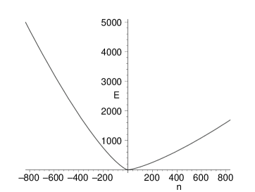
Figure (7) shows the comparison of the discrete evolution of the model with the exact solution of the continuum theory. As we see the discrete theory approximates the continuum theory very well.

,

Figure 7: The discrete evolution of the triad $E$ and the connection $A$ as a function of the discrete evolution parameter $n$. We have chosen initial conditions that produce a positive branch of $A$ for $n>0$ and a negative branch for $n<0$. For the triad we chose both branches positive.

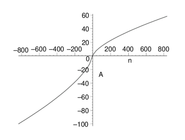
Figure (8) blows up the region of the evolution close to the singularity. As it can be seen the discrete theory evolves through the singularity. Emerging on the other side the evolution has a different value for the lapse and therefore a different time-step. This could be used to implement the proposal of Smolin that physical constants change when one tunnels through the singularity (in lattice theories the lattice spacing determines the “dressed” value of physical constants). See smolin for further discussion of this point.

Figure 8: The approach to the singularity in the discrete and continuum solutions. The discrete theory has a small but non-vanishing triad at $n=0$ and the singularity is therefore avoided.

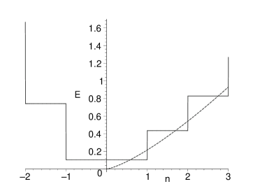
To quantize the theory one has to implement the equations of evolution via a unitary transformation. Details of the derivation can be found in cosmo . The result is

$$<A_{1},\phi_{1},n||A_{2},\phi_{2},n+1> = \delta(\phi_{1}-\phi_{2})\exp\left(i{{\rm sgn}(A_{1})A_{2}^{2}(A_{1}-A_{2})\over\Theta}\right)\sqrt{{|A_{1}|\over\pi\Theta}}.$$ (56)

It should be noted that not all canonical transformations correspond to unitary evolutions at the quantum level. If the canonical transformation defines an isomorphism between the phase spaces at levels $n$ and $n+1$, then one can show that the canonical transformation can be implemented by an isometry at a quantum level. If the isomorphism is an automorphism then the canonical transformation can be implemented as a unitary transformation. A good discussion of canonical transformations in quantum mechanics can be found in Anderson Anderson .

With the unitary transformation introduced above one can answer any question about evolution in the Heisenberg picture for the model in question. One could also choose to work in the Schrödinger picture, evolving the states. Notice that the wavefunctions admit a genuine probabilistic interpretation. This is in distinct contrast with the usual “naive Schrödinger interpretation” of quantum cosmology which attempted to ascribe probabilistic value to the square of a solution of the Wheeler–DeWitt equation (see Kuchar for a detailed discussion of the problems associated with the naive interpretation).

An interesting aspect of this quantization is that for any square-integrable wavefunction and for any value of the parameter $n$, the expectation value of $(P^{A}_{n})^{2}$, and therefore that of $E^{2}$ is non-vanishing, and so are the metric and the volume of the slice. Therefore quantum mechanically one never sees a singularity. The mechanism for elimination of the singularity is quite distinct from the one encountered in loop quantum cosmology Bojowald . The reader may ask how generic is our mechanism. Are singularities always avoided? Singularities are avoided (simply because the a lattice point generically will not coincide with them) provided that they do not occur at a boundary of the phase space. If they occur at a boundary, it is guaranteed that a lattice point will coincide with the singularity and therefore it will not be avoided. In the example we showed the singularity does not occur on the boundary. However, it appears this is a special feature of the large mass approximation in the scalar field. For other models we have studied, at least worked out in the Ashtekar variables, the connection diverges at the singularity and therefore the singularity is at one boundary of the phase space. This can be remedied by changing variables before discretizing so that the singularity is not on a boundary, but it is not what is the direct outcome of discretizing the theory in the Ashtekar variables. An alternative that also eliminates the singularity is to rewrite things in terms of holonomic variables as is done in loop quantum cosmology.

As we will discuss in the next section, it is more desirable to introduce a quantization that is relational in nature. This is because the evolution parameter $n$ cannot be observed physically and therefore is not a good choice of time to have a quantization that is physical. Having implemented the evolution equations as a unitary transformation and having a probabilistic interpretation for the wavefunctions is all that is needed to work out a relational quantization in detail without any of the conceptual problems that were encountered in the past (see Page and Wootters PaWo and the critique of their work by Kuchař Kuchar ).

To define a time we therefore introduce the conditional probabilities, “probability that a given variable have a certain value when the variable chosen as time takes a given value”. For instance, taking $A$ as our time variable, let us work out first the probability that the scalar field conjugate momentum be in the range $\Delta P^{\phi}=[P^{\phi}_{(1)},P^{\phi}_{(2)}]$ and “time” is in the range $\Delta A=[A_{(1)},A_{(2)}]$ (the need to work with ranges is because we are dealing with continuous variables). We go back to the naive quantization and recall that the wavefunction $\Psi[A,\phi,n]$ in the Schrödinger representation admits a probabilistic interpretation. One can also define the amplitude $\Psi[A,P^{\phi},n]$ by taking the Fourier transform. Therefore the probability of simultaneous measurement is,

$$P_{\rm sim}(\Delta P^{\phi},\Delta A)=\lim_{N\to\infty}{1\over N}\sum_{n=0}^{N}\int_{P^{\phi}_{(1)},A_{(1)}}^{P^{\phi}_{(2)},A_{(2)}}\Psi^{2}[A,P^{\phi},n]dP^{\phi}dA.$$ (57)

We have summed over $n$ since there is no information about the “level” of the discrete theory at which the measurement is performed, since $n$ is just a parameter with no physical meaning. With the normalizations chosen if the integral in $P^{\phi}$ and $A$ were in the range $(-\infty,\infty)$, $P_{\rm sim}$ would be equal to one.

To get the conditional probability $P_{\rm cond}(\Delta P^{\phi}|\Delta A)$, that is, the probability that having observed $A$ in $\Delta A$ we also observe $P^{\phi}$ in $\Delta P^{\phi}$, we use the standard probabilistic identity

$$P_{\rm sim}(\Delta P^{\phi},\Delta A)=P(\Delta A)P_{\rm cond}(\Delta P^{\phi}|\Delta A)$$ (58)

where $P(\Delta A)$ is obtained from expression (57) taking the integral on $P^{\phi}$ from $(-\infty,\infty)$. We therefore get

$$P_{\rm cond}(\Delta P^{\phi}|\Delta A)={\lim_{N\to\infty}{1\over N}\sum_{n=0}^{N}\int_{P^{\phi}_{(1)},A_{(1)}}^{P^{\phi}_{(2)},A_{(2)}}\Psi^{2}[A,P^{\phi},n]dP^{\phi}dA\over\lim_{N\to\infty}{1\over N}\sum_{n=0}^{N}\int_{-\infty,A_{(1)}}^{\infty,A_{(2)}}\Psi^{2}[A,P^{\phi},n]dP^{\phi}dA}.$$ (59)

Notice that all the integrals are well defined and the resulting quantity behaves as a probability in the sense that integrating from $(-\infty,\infty)$ in $P^{\phi}$ one gets unity.

Introducing probabilities is not enough to claim to have completed a quantization. One needs to be able to specify what happens to the state of the system as a measurement takes place. The most natural reduction postulate is that,

$$|\psi>\rightarrow{\Pi_{P^{\phi},A}|\phi>\over\sqrt{|<\phi|\Pi_{P^{\phi},A}|\phi>|}},$$ (60)

where

$$\Pi_{P^{\phi},A}=\sum_{n=0}^{N}|P^{\phi},A,n><P^{\phi},A,n|.$$ (61)

The model considered is too simple to test too much of the framework, however, we have shown that one can work out in detail the discrete treatment at a classical an quantum mechanical level without conceptual obstructions. It is a big leap to claim that because everything worked well for such a simple model these ideas will succeed in full GR. Currently we are working in detail the discretization of Gowdy cosmologies, which have field theoretic degrees of freedom. Recently achieved success Gowdy in such models greatly enhances our confidence in the ability of this scheme to discretize general relativity.

For now, we would like to take a glimpse at some possibilities that the framework will introduce in the full theory, we do so in the next section.

V Applications in quantum gravity

Having made the case that one can approximate general relativity by a discrete theory that is constraint-free allows us to make progress in many aspects of quantum gravity. Most of the hard conceptual problems that one faces in canonical quantum gravity are related to the presence of constraints in the theory. For an unconstrained theory, most obstructions are eliminated. One of the first obstructions we can deal with is the “problem of time”. To a certain extent we have shown that this is possible in Rovelli’s example (which has a “problem of time”) and in the cosmological model. But actually progress is possible in a more generic sense. One can, for instance, implement the relational time that was proposed by Page and Wootters PaWo in the full theory. The idea consists in quantizing the theory by promoting all variables to quantum operators, unlike the usual Schrödinger quantization in which a variable called “time” is kept classical. One then picks from among the quantum operators one that we will call “clock”. It should be emphasized that it is a quantum operator and therefore will have an expectation value, fluctuations, etc. One then computes conditional probabilities for the other variables in the theory to take certain values when the “clock” variable has a given value.

The resulting conditional probabilities do not evolve according to a Schrödinger equation. If one chooses as “clock” a variable that behaves close to classicality (small fluctuations) then one can show that the conditional probabilities evolve approximately by a Schrödinger evolution. But as the fluctuations in the clock variable increase there appear corrective terms in the evolution equations. The fist kind of corrective terms were evaluated in GaPoPunjp and have the form of a Lindblad type of evolution. A feature of the evolution implied by the use of “real clocks” as we are considering is that it is not unitary. In general pure states evolve into mixed states. This is easy to understand in our discrete approach. There we saw that evolution in terms of the discrete parameter $n$ was implemented by a canonical transformation. Upon quantization evolution is implemented by a unitary operator. However, the real clock variable we choose will in general have a probability distribution with a certain spread in $n$. If evolution is unitary in $n$ then it cannot be unitary in the clock variable since in general for a given value of the clock variable one will have a superposition of states with different values of $n$.

This lack of unitarity could in principle be experimentally observable. We have estimated its magnitude in GaPoPuprl . In order to make an estimate one needs to make a model of what is the “most classical” clock one can construct. To do this we borrowed from ideas of Ng and Van Dam, Amelino-Camelia and more recently Lloyd and collaboratorsngac . They start with the observation of Salecker and Wigner SaWi that the accuracy of a clock is limited by its mass $\delta T>\sqrt{T/M}$ (in units of $\hbar=c=1$) where $T$ is the time to be measured. Then they argue that the maximum amount of mass one can concentrate can be achieved in a black hole. If the clock is a black hole its accuracy is given by its quasinormal frequencies, $\delta T>T_{P}^{2}M$. where $T_{P}$ is Planck’s time. Combining the two inequalities we get, $\delta T\sim T_{P}\sqrt[3]{T/T_{P}}$

If one now considers a model system consisting of two quantum mechanical levels and estimates the lack of coherence induced by the use of the relational time one finds that it that the elements of the density matrix that are off-diagonal in the energy basis decay exponentially. The exponent is given by $t_{P}^{(4/3)}T^{(2/3)}\omega_{12}^{2}$ where $T$ is the time we observe the system and $\omega_{12}$ is the Bohr frequency between both levels. Given the presence of the $t_{P}$ factor, this effect is unobservable for almost all experimental situations. An exception could be “macroscopic” quantum states, like the ones that are starting to become available through Bose-Einstein condensates. Current technology does not produce states that are “macroscopic enough” for the effect to be observable, and it remains to be seen if future technologies could produce such states (and keep them free of ambiental decoherence effects) for this effect to be observable (for an independent discussion see SiJa .

One place where the fundamental decoherence could play a role is in the black hole information puzzle. Black holes take a very long time to evaporate and therefore there is a chance for the decoherence to build up. The question is: does it build up enough to wipe out all coherence from the states before the black hole would have done the same via Hawking evaporation? We recently estimated the effect by considering a very naive model of a black hole consisting of two energy levels separated by $kT$ with k the Boltzmann constant and $T$ the temperature predicted by Hawking for the black hole. We found out that piombino

$$|\rho_{12}(T_{\rm max})|\sim|\rho_{12}(0)|\left({M_{\rm Planck}\over M_{\rm BH}}\right)^{2\over 3}$$ (62)

where $\rho_{12}$ is an off-diagonal element of the density matrix of the state of interest at the time the black hole would have evaporated. For a Solar sized black hole the magnitude of the off diagonal element is $10^{-28}$, that is, it would have de facto become a mixed state even before invoking the Hawking effect. The information paradox is therefore unobservable in practice. It should be noted that this estimate is an optimistic one. In reality clocks fare much worse than the estimate we worked out and the fundamental decoherence will operate even faster than what we consider here.

VI Connections with continuum loop quantum gravity

In spite of the possibilities raised by the discrete approach, some readers may feel that it forces us to give up too much from the outset. This was best perhaps captured by Thomas Thiemann Thiemann , who said “While being a fascinating possibility, such a procedure would be a rather drastic step in the sense that it would render most results of LQG obtained so far obsolete”. Indeed, the kinematical structure built in loop quantum gravity, with a rigorous integration measure and the natural basis of spin foam states appear as very attractive tools to build theories of quantum gravity. We would like to discuss how to recover these structures in our discrete approach.

To make contact with the traditional kinematics of loop quantum gravity, we consider general relativity and discretize time but keep space continuous, and we proceed as in the consistent discretization approach, that is, discretizing the action and working out the equations of motion. We start by considering the action written in terms of Ashtekar variables asle ,

$$S=\int dtd^{3}x\left(\tilde{P}^{a}_{i}F_{0a}^{i}-N^{a}C_{a}-NC\right)$$ (63)

where $N,N^{a}$ are Lagrange multipliers, $\tilde{P}^{a}_{i}$ are densitized triads, and the diffeomorphism and Hamiltonian constraints are given by, $C^{a}=\tilde{P}^{a}_{i}F_{ab}^{i}$, $C={\tilde{P}^{a}_{i}\tilde{P}^{b}_{j}\over\sqrt{\rm det}q}\left(\epsilon^{ijk}F_{ab}^{i}-(1+\beta^{2})K_{[a}^{i}K_{b]}^{j}\right)$ where $\beta K_{a}^{i}\equiv\Gamma_{a}^{i}-A_{a}^{i}$ and $\Gamma_{a}^{i}$ is the spin connection compatible with the triad, and $q$ is the three metric. We now proceed to discretize time. The action now reads,

$$S = \int dtd^{3}x\left[{\rm Tr}\left(\tilde{P}^{a}\left(A_{a}(x)-V(x)A_{n+1,a}(x)V^{-1}(x)+\partial_{a}(V(x))V^{-1}(x)\right)\right)\right.$$

$$\left.-N^{a}C_{a}-NC+\mu\sqrt{\rm det}q{\rm Tr}\left(V(x)V^{\dagger}(x)-1\right)\right]$$

In the above expression $V(x)=V_{I}T^{I}$ is the parallel transport matrix along a time-like direction and $F_{0a}$ is approximated by the holonomy along a plaquette that is finite in the “time-like” direction and infinitesimal in the “space-like” direction and $T^{0}=1/\sqrt{2}$ and $T^{a}=-i\sigma^{a}/\sqrt{2},a=1..3$ and $\sigma$’s are the Pauli matrices and the coefficients $V_{I}$ are real. We have omitted the subscript $n$ to simplify the notation and kept it in the quantities that are evaluated at $n+1$. The last term involves a Lagrange multiplier $\mu$ and is present in order to enforce the fact that the parallel transport matrices are unitary. We notice that the $SU(2)$ gauge invariance is preserved in the semi-discrete theory. This in turn implies that Gauss’ law for the momentum canonically conjugate to the connection, $\tilde{E}^{a}_{n+1}\equiv V^{-1}\tilde{P}^{a}V$ is preserved automatically upon evolution. Remarkably, although the theory does not have a diffeomorphism constraint, one can show that the quantity that in the continuum would correspond to the diffeomorphism constraint is a conserved quantity (to intuitively see this, notice that the action is invariant under (time independent) spatial diffeomorphisms and $n$ and $n+1$). One can then impose that this quantity vanish and this requirement is consistent with evolution. One would therefore have a theory with the same constraints as kinematical loop quantum gravity and with an explicit evolution scheme as is usual in consistently discretized theories.

In reference difeo we have actually worked out the procedure in detail for the case of $2+1$ dimensions, treating gravity as a BF theory. The procedure reproduces the physical space for the theory of traditional quantizations.

Summarizing, one can apply the consistent discretization approach by discretizing only time. The resulting theory has no constraints, but the diffeomorphism constraint can be introduced additionally, so the resulting theory has the same kinematics as loop quantum gravity. The dynamics is implemented via a unitary operator. As in the full discrete approach, one can envision bypassing many of the hard conceptual questions of canonical quantum gravity, for instance introducing a relational notion of time. This can actually be seen as a concrete framework to implement loop quantum gravity numerically, since it is not expected that one will be able to work out things analytically in the full case.

VII Conclusions

The consistent discretization approach is emerging as an attractive technique to handle discrete general relativity, both at a classical and at a quantum mechanical level. In quantum gravity, since it does away with the constraints it solves in one sweep some of the hardest conceptual issues of canonical quantization. In classical general relativity there is a growing body of evidence that suggests that the discretizations work numerically and approximate the continuum theory (including its constraints) in a convergent and stable way. Having discrete theories with these properties classically is a desirable point of view for any effort towards quantization. The discrete approach also yields directly computable evolutions quantum mechanically opening the possibility for concrete numerical quantum gravity calculations.

VIII Acknowledgements

This work was supported in part by grants NSF-PHY0244335, and by funds of the Horace C. Hearne Jr. Institute for Theoretical Physics and CCT-LSU.

References

- (1) A. Lew, J. Marsden, M. Ortiz, M. West, in “Finite element methods: 1970’s and beyond”, L. Franca, T. Tezduyar, A. Masud, editors, CIMNE, Barcelona (2004).
- (2) R. McLachlan, M. Perlmutter “Integrators for nonholonomic mechanical systems” preprint (2005).
- (3) C. Di Bartolo, R. Gambini, J. Pullin, Class. Quan. Grav. 19, 5275 (2002).
- (4) R. Gambini and J. Pullin, Phys. Rev. Lett. 90, 021301, (2003).
- (5) C. Di Bartolo, R. Gambini, R. Porto and J. Pullin, J. Math. Phys. 46, 012901 (2005) [arXiv:gr-qc/0405131].
- (6) C. Rovelli, Phys. Rev. D 42, 2638 (1990).
- (7) R. Gambini and J. Pullin, Class. Quant. Grav. 20, 3341 (2003) [arXiv:gr-qc/0212033].
- (8) R. Gambini and J. Pullin, Int. J. Mod. Phys. D 12, 1775 (2003) [arXiv:gr-qc/0306095].
- (9) A. Anderson, Annals Phys. 232,292-331 (1994) [arXiv:hep-th/9305054].
- (10) K. Kuchař, “Time and interpretations of quantum gravity”, in “Proceedings of the 4th Canadian conference on general relativity and relativistic astrophysics”, G. Kunstatter, D. Vincent, J. Williams (editors), World Scientific, Singapore (1992). Available online at http://www.phys.lsu.edu/faculty/pullin/kvk.pdf
- (11) M. Bojowald, Pramana 63, 765 (2004)
- (12) D. N. Page and W. K. Wootters, Phys. Rev. D 27, 2885 (1983); W. Wootters, Int. J. Theor. Phys. 23, 701 (1984); D. N. Page, “Clock time and entropy” in “Physical origins of time asymmetry”, J. Halliwell, J. Perez-Mercader, W. Zurek (editors), Cambridge University Press, Cambridge UK, (1992).
- (13) R. Gambini, M. Ponce, J. Pullin, “Consistent discretizations of Gowdy cosmologies” (in preparation).
- (14) R. Gambini, R. Porto and J. Pullin, New J. Phys. 6, 45 (2004) [arXiv:gr-qc/0402118].
- (15) R. Gambini, R. A. Porto and J. Pullin, Phys. Rev. Lett. 93, 240401 (2004) [arXiv:hep-th/0406260].
- (16) G. Amelino-Camelia, Mod. Phys. Lett. A 9, 3415 (1994) [arXiv:gr-qc/9603014]; Y. J. Ng and H. van Dam, Annals N. Y. Acad. Sci. 755, 579 (1995) [arXiv:hep-th/9406110]; Mod. Phys. Lett. A 9, 335 (1994); V. Giovanetti, S. Lloyd, L. Maccone, Science 306, 1330 (2004); S. Lloyd, Y. J. Ng, Scientific American, November 2004.
- (17) E. Wigner, Rev. Mod. Phys. 29, 255 (1957); H. Salecker, E. Wigner, Phys. Rev. 109, 571 (1958).
- (18) C. Simon and D. Jaksch, Phys. Rev. A70, 052104 (2004) [arXiv:quant-ph/0406007].
- (19) R. A. Gambini, R. Porto and J. Pullin, “Fundamental decoherence in quantum gravity,”, to appear in the proceedings of 2nd International Workshop DICE2004: From Decoherence and Emergent Classicality to Emergent Quantum Mechanics, Castello di Piombino, Tuscany, Italy, 1-4 Sep 2004, H. T. Elze, editor [arXiv:gr-qc/0501027].
- (20) T. Thiemann, “The Phoenix project: Master constraint programme for loop quantum gravity,” arXiv:gr-qc/0305080.
- (21) A. Ashtekar, J. Lewandowski Class. Quant. Grav. 21, R53 (2004) [arXiv:gr-qc/0404018].
- (22) R. Gambini and J. Pullin, Phys. Rev. Lett. 94, 101302 (2005) [arXiv:gr-qc/0409057].