Gowdy $T^{3}$ Cosmological Models in $N=1$ Supergravity

Abstract

We investigate the canonical quantization of supergravity $N=1$ in the case of a midisuperspace described by Gowdy $T^{3}$ cosmological models. The quantum constraints are analyzed and the wave function of the universe is derived explicitly. Unlike the minisuperspace case, we show the existence of physical states in midisuperspace models. The analysis of the wave function of the universe leads to the conclusion that the classical curvature singularity present in the evolution of Gowdy models is removed at the quantum level due to the presence of the Rarita-Schwinger field.

File: gowsg2.tex; 30.03.2005

I Introduction

Supergravity was originally developed as an elementary field theory which should avoid the ultraviolet divergencies and consequently would represent the long awaited unification of gravity with the remaining fundamental interactions of nature. Supersymmetry plays an important role in the development of unification models beyond the standard model of elementary particles, in the formulation of the conceptual fundamentals of quantum field theory and quantum gravity, and more recently in the understanding of important aspects of superstring theory (see, for instance, reviews1 for reviews of the conceptual basis of supersymmetry and supergravity). Today, supergravity is considered in the first place as an effective field theory which should describe the low-mass degrees of freedom of a more fundamental theory, probably the still unknown M-theory; however, at the moment the only known candidate for such a theory is superstring theory (see, for example, reviews2 ).

The classical field equations following from the $N=1$ supergravity Lagrangian were derived in pi78 by using the Hamiltonian formalism. There are constraints for each of the gauge symmetries contained in the theory: spacetime diffeomorphisms, local Lorentz invariance, and supersymmetry. One important result that follows from the analysis of the field equations is that one of the constraints relates the torsion tensor and the Rarita-Schwinger field so that it can be used to eliminate the torsion tensor from the theory.

The canonical quantization of supergravity is performed in general by applying Dirac’s procedure for constrained systems. One uses the 3+1 decomposition of the canonical theory to obtain a Hamiltonian in which the symmetry generators of the gauge fields are constrained by Lagrange multipliers. Then it is postulated that the wave function is annihilated by all the constraints. In the case of $N=1$ supergravity there are three constraints: the Hamiltonian constraint, the generators of Lorentz rotations and the supersymmetric constraint. It turns out tei77 that the Hamiltonian constraint is identically satisfied once the supersymmetric constraint is fulfilled. Accordingly, only the Lorentz and supersymmetric constraints are the central issue.

The study of $N=1$ supergravity models has been limited so far to minisuperspace models ho ; gc ; gc2 ; pde ; opr ; maoso ; mms98 ; mac99 as direct generalizations of quantum cosmology models. The standard approach to quantum cosmology consists in canonically quantizing a minisuperspace model which is obtained by imposing certain symmetry conditions on the metrics allowed on the spacelike slices of the universe. This procedure, however, reduces the number of degrees of freedom to a finite number and the problem of quantization can be attacked by applying the canonical methods of quantum mechanics qc ; ryan . The dynamics of the system is governed by the Wheeler-DeWitt equation which is a second order differential constraint equation following from general covariance, and acts on the wave function of the universe. The most general minisuperspace models analyzed in the literature correspond to homogeneous and anisotropic Bianchi cosmological models. Since the corresponding metrics depend only on time, the dynamics of the spacelike 3-dimensional slices becomes trivial, unless an additional reparametrization is performed. Usually, in the reparametrization one of the scale factors of the Bianchi metric is taken as “internal time” so that the Wheeler-DeWitt equation generates a wave function of the universe which explicitly depends on the internal time and the remaining scale factors. Although this is a quite elegant procedure which in each case leads to an explicit wave function of the universe, the main problem regarding the existence of classical initial singularity remains unsolved. In fact, in all analyzed minisuperspaces the classical singularity remains at the quantum level. Moreover, the original hope that the behavior of minisuperspace models would hold at least qualitatively in the full theory seems to be not realized. In fact, in kucryan it was shown that even in the simple case of a microsuperspace (a reduced minisuperspace) contained in the seed minisuperspace the behavior of the corresponding wave functions is widely different. The problem of the initial classical singularity has been attacked alternatively by proposing a wave function for the ground state harhaw or a tunneling effect vil84 , among other proposals. In both cases the main idea consists in replacing the classical singularity by an ad hoc postulated universe. The initial singularity problem remains thus unsolved. The consideration of an additional Rarita-Schwinger field in the context of supergravity minisuperspace models (supersymmetric quantum cosmology) does not solve the problem, and the classical singularity remains.

In all the cases the failure to solve the singularity problem can be attributed to the fact that, due to the strong symmetry reduction, only a finite number of degrees of freedom can be considered. To face this difficulty one needs to analyze genuine field theories with an infinite number of degrees of freedom. An option would be to consider milder symmetry reductions which leave unaffected a specific set of true local degrees of freedom. These are the so called midisuperspace models. Such spacetimes have a long history in general relativity. Indeed, any spacetime which allows the existence of two commuting Killing vector fields leads to a real field theory with an infinite number of degrees of freedom. The field equations in this case can be shown to be equivalent to the wave equation for a scalar field propagating in a fictitious flat 2+1-dimensional spacetime krameretal . The local degrees of freedom are contained in the scalar field.

In this work we will consider the specific midisuperspace described by Gowdy $T^{3}$ cosmological models gow71 ; gow74 in the context of $N=1$ supergravity. We will find an explicit expression for the wave function of the universe and will show that the mere consideration of a genuine field theory leads to a solution of the singularity problem. In fact, the singular behavior of Gowdy models at a certain time of their evolution has been investigated in detail at the classical level. It has been shown that the behavior of the metric near the singularity corresponds to the so called “asymptotically velocity term dominated” (AVTD) behavior (see, for instance ber02 , for a recent review). We will see that the AVTD singular behavior disappears at the level of the corresponding wave function of the universe.

This paper is organized as follows. In Section II we revise the canonical formulation of supergravity $N=1$ and analyze the Lorentz constraint, following closely notations and conventions of mamilo . In Section III we present the Gowdy $T^{3}$ cosmological models and their main properties. Section IV is devoted to the investigation of the supersymmetric constraint and the solutions for the wave function of the universe. Finally, Section V contains several final remarks and the conclusions with indications about different possibilities of generalizing the results derived in this work.

We adopt the following conventions and notations. Indices related to world coordinates are denoted by Greek letters. The ones from the middle of the alphabet, i. e. $\mu,\ \nu,...$, run over 0,1,2,3 and the ones from the beginning of the alphabet, i. e. $\alpha,\ \beta,...$, represent only spatial coordinates 1,2,3. Capital Latin indices, i.e. $A,\ B,...$ can take the values 0,1,2,3 and the small ones run over 1,2,3; both of them refer to to components in an orthonormal local frame, for which we use the local metric $\eta_{AB}={\rm diag}(+,-,-,-)$.

II Canonical formulation of $N=1$ supergravity

The fields of $N=1$ supergravity in 4 dimensions are the vierbein $e_{\mu}^{\ A}$ and the Rarita-Schwinger gravitino $\psi_{\mu}$, which is a vector of Majorana spinors. The corresponding Lagrangian is given by

$${\cal{L}}=\frac{1}{2}\sqrt{-g}R-\frac{i}{2}\epsilon^{\lambda\mu\nu\rho}\bar{\psi}_{\lambda}\gamma_{5}\gamma_{\mu}D_{\mu}\psi_{\rho}\,,$$ (1)

where

$$D_{\nu}=\partial_{\nu}+\frac{1}{2}\omega_{\nu AB}\sigma^{AB}\,,$$ (2)

is the covariant derivative with the Lorentz generators $\sigma^{AB}=(1/4)(\gamma^{A}\gamma^{B}-\gamma^{B}\gamma^{A})$. For the $\gamma^{A}$ matrices we use the real Majorana representation

$$\gamma^{0}=\left(\begin{array}[]{cc}0&\sigma^{2}\\ \sigma^{2}&0\end{array}\right)\,,\,\,\gamma^{1}=\left(\begin{array}[]{cc}i\sigma^{3}&0\\ 0&i\sigma^{3}\end{array}\right)\,,\,\,\gamma^{2}=\left(\begin{array}[]{cc}0&-\sigma^{2}\\ \sigma^{2}&0\end{array}\right)\,,\,\,\gamma^{3}=\left(\begin{array}[]{cc}-i\sigma^{1}&0\\ 0&-i\sigma^{1}\end{array}\right)\,,$$ (3)

in which the anticommutator relation $\{\gamma^{A},\gamma^{B}\}=2\eta^{AB}$ is satisfied, and $\sigma^{i}$ are the standard Pauli matrices. Moreover, $\gamma_{5}=i\gamma^{0}\gamma^{1}\gamma^{2}\gamma^{3}$. In this representation ${\overline{\psi}}=-i\psi^{T}\gamma^{0}$ is known as the Majorana condition. The (endomorphic) components of the Ricci rotation coefficients can be obtained from Cartan’s first structure equation ${d}e^{A}=-\omega^{A}_{\ B}\wedge e^{B}$, and $\omega_{AB}=\omega_{\mu AB}{d}x^{\mu}$. Notice that in general the Ricci rotation coefficients contain a contorsion term. However, as we mentioned in the introduction the torsion tensor can be eliminated from the theory by using one of the constraint equations.

Applying the canonical 3+1 decomposition of spacetime pi78 the canonical variables can be chosen to be the spatial components of the tetrad vectors $e^{a}_{\ \alpha}$, their conjugate momenta $p_{a}^{\ \alpha}$, and the spatial covariant components of the spinor $\psi_{\alpha}$. In this case, the corresponding temporal components turn out to be Lagrange multipliers of the Hamiltonian which contains only the constraints associated with the three different types of symmetries of the system:

$$H=e^{A}{}_{0}\,{\cal H}_{A}+\frac{1}{2}\omega_{0}{}^{AB}\,{\cal J}_{AB}+{\overline{\psi}}_{0}\,{\cal S}\,,$$ (4)

Here ${\cal H}_{A}$ contains the usual Hamiltonian and diffeomorphisms constraints, ${\cal J}_{AB}$ is the Lorentz constraint and ${\cal S}$ denotes the supersymmetric constraint. According to Dirac’s canonical quantization procedure for constrained systems, the physical states $|\Psi\rangle$ must be annihilated by the corresponding constraint operators, i.e.

$${\cal S}|\Psi\rangle=0\,,\qquad{\cal H}_{A}|\Psi\rangle=0\,,\qquad{\cal J}_{AB}|\Psi\rangle=0\,.$$ (5)

From the fact that the supergravity operators satisfy Teitelboim’s algebra tei77 it follows that the condition ${\cal H}_{A}|\Psi\rangle=0$ is satisfied identically once ${\cal S}|\Psi\rangle=0$ is fulfilled. Consequently, we need to consider only the Lorentz and supersymmetric constraints.

It is convenient to use, instead of the gravitino field, the densitized local components ($\psi_{0}$ is a Lagrange multiplier and so is $\phi_{0}$ )

$$\phi_{a}=e\,e_{a}{}^{\alpha}\psi_{\alpha}\,,$$ (6)

as the basic fields commuting with all non–spinor variables, where $e={}^{(3)}e=\det(e_{a}{}^{\alpha})$. Moreover, if we choose an $SO(3)$ basis it is possible to show that all bosonic terms of the Lorentz constraint cancel each other, yielding pi78

$${\cal J}_{AB}=\frac{1}{2}\phi_{[A}^{T}\phi_{B]}\,,$$ (7)

and the generator of supersymmetry is given by

$${\cal S}=\varepsilon^{0\alpha\beta\delta}\gamma_{5}\gamma_{\alpha}D_{\beta}\psi_{\delta}\,,$$ (8)

where a factor ordering is usually chosen mor .

Let us first analyze the Lorentz condition ${\cal J}_{AB}|\Psi\rangle=0$ that explicitly reads

$${\cal J}_{AB}|\Psi\rangle=\left(\begin{array}[]{cccc}0&0&0&0\\ 0&~{}0&~{}{\cal J}_{12}&~{}{\cal J}_{13}\\ 0&~{}-{\cal J}_{12}&~{}~{}0&~{}{\cal J}_{23}\\ 0&~{}-{\cal J}_{13}&~{}-{\cal J}_{23}&~{}~{}0\end{array}\right)\left(\begin{array}[]{c}\Psi_{I}\\ \Psi_{II}\\ \Psi_{III}\\ \Psi_{IV}\end{array}\right)=0\,.$$ (9)

Since this constraint does not affect the component $\Psi_{I}$, a particular solution is to keep $\Psi_{I}$ arbitrary and

$$\Psi_{II}=\Psi_{III}=\Psi_{IV}=0.$$ (10)

This is the “rest-frame” solution kaku in which only the component $\Psi_{I}$ remains to be determined by the supersymmetric constraint. If none of the conditions (10) is satisfied, the Lorentz constraint implies that Niew81

$${\cal J}_{12}\Psi_{III} = -{\cal J}_{13}\Psi_{IV}\,,$$ (11)

$${\cal J}_{12}\Psi_{II} = {\cal J}_{23}\Psi_{IV}\,,$$ (12)

$${\cal J}_{13}\Psi_{II} = -{\cal J}_{23}\Psi_{III}\,.$$ (13)

Notice that in the representation we are using here the Lorentz generators ${\cal J}_{ab}$ are $4\times 4$ matrices. Therefore, the components $\Psi_{I},\ \Psi_{II},\ \Psi_{III}$, and $\Psi_{IV}$ of the wave function must be considered as $4\times 1$ matrices.

There are two alternative ways to solve the system of algebraic equations given in (11)–(13). The first one consists in taking the components $\Psi_{II},\ \Psi_{III}$, and $\Psi_{IV}$ proportional to each other. The proportionality factors can be absorbed by redefining each component of the wave function so that this case can be written as

$$\Psi_{II}=\Psi_{III}=\Psi_{IV}\ .$$ (14)

Then from Eqs.(11)-(13) it follows that

$${\cal J}_{12}=-{\cal J}_{13}={\cal J}_{23}\ ,$$ (15)

a condition which implies a trivialization of the Lorentz constraint. Then from the expression (7) we can determine the components of the gravitino field. In the trivial case (15) we obtain

$$\phi_{1}=-\phi_{2}=\phi_{3}\ .$$ (16)

The second possibility is to solve explicitly the system of equations (11)–(13). The relation between the components of the Lorentz generators can be solved by representing each component as a product of $\gamma$-matrices, under the condition that the corresponding Lorentz algebra is preserved. Alternatively we can use the standard generators of the ordinary rotation group $O(3)$ as given in kaku

$${\cal J}_{12}=-i\left(\begin{array}[]{cccc}0&0&0&0\\ 0&0&1&0\\ 0&-1&0&0\\ 0&0&0&0\end{array}\right)\,,{\cal J}_{13}=i\left(\begin{array}[]{cccc}0&0&0&0\\ 0&0&0&-1\\ 0&0&0&0\\ 0&1&0&0\end{array}\right)\,,\,\,{\cal J}_{23}=-i\left(\begin{array}[]{cccc}0&0&0&0\\ 0&0&0&0\\ 0&0&0&1\\ 0&0&-1&0\end{array}\right)\,.$$ (17)

Solving explicitly the Lorentz constraint (11)–(13) in this representation it is easy to see that for each of the vectors $\Psi_{II}$, $\Psi_{III}$, $\Psi_{IV}$ only one component is different from zero. That is to say the wave function of the universe can be represented as

$$|\Psi\rangle=\left(\begin{array}[]{c}\Psi_{I}\\ \Psi_{II}\\ \Psi_{III}\\ \Psi_{IV}\end{array}\right)=E\left(\begin{array}[]{c}{\bf a}_{0}\\ b_{0}\\ c_{0}\\ d_{0}\end{array}\right)\,,$$ (18)

where $E$ is a function to be determined, ${\bf a}_{0}$ is an arbitrary 4–vector and $b_{0}$, $c_{0}$, and $d_{0}$ are arbitrary constants. For the sake of simplicity later on we will consider the special case ${\bf a}_{0}=\{a_{0},0,0,0\}$. So we have shown that the wave function (18) explicitly solves the Lorentz constraint. The remaining function $E$ and the arbitrary constants $a_{0}$, $b_{0}$, $c_{0}$, and $d_{0}$ have to be chosen so that the supersymmetric constraint is satisfied.

This ends the analysis of the Lorentz constraint. Notice that in the “rest-frame” solution (10), the wave function of the universe is a scalar with only one independent component. For the further investigation of this solution as well as of the non-trivial solution (14), we need to analyze the supersymmetric constraint (8), in which the bosonic part plays a prominent role. In the next Section we will present the specific gravitational field which completely determines the bosonic part of the supersymmetric constraint.

III Gowdy $T^{3}$ cosmological models

Gowdy cosmological models are inhomogeneous time-dependent solutions of Einstein’s vacuum equations with compact Cauchy spatial hypersurfaces whose topology can be either $T^{3}$ or $S^{1}\times S^{2}$ gow71 ; gow74 . Other particular topologies are contained in these two as special cases. Here we will focus on $T^{3}$ models for which the line element can be written as

$$ds^{2}=e^{-\lambda/2+\tau/2}(e^{-2\tau}d\tau^{2}-d\chi^{2})-e^{-\tau}\left[e^{P}(d\sigma+Qd\delta)^{2}+e^{-P}d\delta^{2}\right]\ ,$$ (19)

where $P$, $Q$, and $\lambda$ depend on the non-ignorable coordinates $\tau$ and $\chi$. The spatial hypersurfaces $(\tau=$const) are compact if we require that $0\leq\chi,\sigma,\delta\leq 2\pi$. The expression in square brackets depicts the metric on the $T^{2}$ subspace which is generated by the commuting Killing vectors $\partial_{\sigma}$ and $\partial_{\delta}$. The coordinate $\chi$ labels the several tori.

When the Killing vectors are hypersurface orthogonal, the general line element (19) becomes diagonal with $Q=0$ and the corresponding cosmological models are called polarized. In this last case, the subspace $T^{2}$ corresponds to the spatial surfaces of a $2+1$ fictitious flat spacetime in which a scalar field, represented by the metric function $P$, propagates ashpierri ; ccq1 . The local degrees of freedom contained in the scalar field are true gravitational degrees of freedom which cannot be eliminated by a choice of gauge. We are thus facing a genuine field theory which is a special case of a midisuperspace model. Notice that the infinite number of degrees of freedom contained in this midisuperspace model can be associated with the inhomogeneous character of the spacetime. If we would neglect the inhomogeneities present in the model, we would obtain a minisuperspace model with a finite number of degrees of freedom, probably related to a Bianchi cosmological model. The general unpolarized case $(Q\neq 0)$ also corresponds to a midisuperspace model; however, its interpretation in terms of a dynamical scalar field in a 2+1 spacetime can not be realized. In this work we will concentrate on the polarized case $(Q=0)$ where the field equations can be integrated in general. The general unpolarized case $(Q\neq 0)$ will be also considered in quite general terms at the level of the wave function of the universe, although no exact solution with $Q\neq 0$ will be analyzed due to the difficulty of the classical field equations.

The vacuum field equations for the general line element (19) can be written as a set of two second order differential equations for $P$ and $Q$

$$P_{\tau\tau}-e^{-2\tau}P_{\chi\chi}-e^{2P}(Q_{\tau}^{2}-e^{-2\tau}Q_{\chi}^{2}) = 0\,,$$ (20)

$$Q_{\tau\tau}-e^{-2\tau}Q_{\chi\chi}+2(P_{\tau}Q_{\tau}-e^{-2\tau}P_{\chi}Q_{\chi}) = 0\,,$$ (21)

and two first order differential equations for $\lambda$

$$\lambda_{\tau} = P_{\tau}^{2}+e^{-2\tau}P_{\chi}^{2}+e^{2P}(Q_{\tau}^{2}+e^{-2\tau}Q_{\chi}^{2})\,,$$ (22)

$$\lambda_{\chi} = 2(P_{\chi}P_{\tau}+e^{2P}Q_{\chi}Q_{\tau})\,.$$ (23)

Notice that the function $\lambda$ can be calculated by quadratures once $P$ and $Q$ are known. The system of differential equations (20) and (21) for $P$ and $Q$ is highly nonlinear, has been investigated in detail by using numerical methods varios , and has been analyzed analytically only recently in oqr1 ; oqr2 ; nosotros where several special solutions have been derived. In the special polarized case, using the method of separation of variables it is possible to find the general solution as

$$Q=0,\ \ P(\tau,\chi)=\sum_{n=0}^{\infty}[A_{n}\cos{(n\chi)}+B_{n}\sin{(n\chi)}][C_{n}J_{0}(ne^{-\tau})+D_{n}N_{0}(ne^{-\tau})]\,,$$ (24)

where $A_{n}$, $B_{n}$, $C_{n}$ and $D_{n}$ are arbitrary constants and $J_{0}$, $N_{0}$ are Bessel functions. The integration of the function $\lambda$ is quite cumbersome for the general solution. We will present in Section IV a particular solution characterized by a finite number of terms of the sum (24).

The behavior of Gowdy cosmological models near the singularity is an important property that has been intensively used to study the geometric behavior of the initial Big-Bang singularity of our Universe. In the case of $T^{3}$ models it can be shown that the singularity is approached in the limit $\tau\rightarrow\infty$. It has been proved that all polarized Gowdy models belong to the class of “asymptotically velocity term dominated” (AVTD) solutions and it has been conjectured that the general (unpolarized) models are also AVTD mon1 . This conjecture has been reinforced through the analogy with other midisuperspaces her . The AVTD behavior states that near the singularity each point in space is characterized by a different spatially homogeneous cosmology eardley . It implies that at the singularity all spatial derivatives of the field equations can be neglected and only the temporal behavior is relevant. This leads to a “truncated” set of differential equations which in the case of $T^{3}$ models can be obtained from Eqs.(20) - (23) by neglecting all the derivatives with respect to the spatial coordinate $\chi$. It is easy to see that the general solution to this “truncated” system is given by Berger ; nosotros

$$P_{AVTD}=\ln[a(e^{-c\tau}+b^{2}e^{c\tau})]\ ,\quad Q_{AVTD}=\frac{b}{a(e^{-2c\tau}+b^{2})}+d\ ,\quad\lambda_{AVTD}=\lambda_{0}+c^{2}\tau\ ,$$ (25)

where $a,\ b,\ c$, $d$, and $\lambda_{0}$ can be considered as arbitrary real constants. The singularity situated at $\tau\rightarrow\infty$ is characterized by a blow up of the curvature which is determined by the behavior of the AVTD solution (25).

For the calculation of the supersymmetric constraint we need explicitly the connection in an orthonormal basis. The structure of the line element (19) suggests the following choice for the vierbein

$$e^{0}=e^{-(\lambda+3\tau)/4}d\tau\,,\quad e^{1}=e^{-(\lambda-\tau)/4}d\chi\,,\quad e^{2}=e^{(P-\tau)/2}(d\sigma+Qd\delta)\,,\quad e^{3}=e^{-(P+\tau)/2}d\delta\,,$$ (26)

which satisfies the orthonormality condition $g^{\mu\nu}e^{A}{}_{\mu}e^{B}{}_{\nu}=\eta^{AB}$ with $e^{A}=e^{A}_{\ \mu}dx^{\mu}$. In this tetrad the non-vanishing components of the connection $\omega_{\mu AB}$ are

$$\omega_{0\hat{0}\hat{1}} = -\frac{1}{4}\lambda_{\chi}\,,\qquad\qquad\qquad~{}\omega_{0\hat{2}\hat{3}}=-\frac{1}{2}e^{\tau+P}Q_{\tau}\,,$$

$$\omega_{1\hat{0}\hat{1}} = -\frac{1}{4}e^{\tau}(1-\lambda_{\tau})\ ,\quad\qquad\omega_{1\hat{2}\hat{3}}=\frac{1}{2}e^{P}Q_{\chi}\ ,$$

$$\omega_{2\hat{0}\hat{2}} = \frac{1}{2}e^{\frac{\tau}{4}+\frac{\lambda}{4}+\frac{P}{2}}(1-P_{\tau})\ ,~{}\quad\omega_{2\hat{3}\hat{0}}=-\frac{1}{2}e^{\frac{\tau}{4}+\frac{\lambda}{4}}Q_{\tau}\ ,$$

$$\omega_{2\hat{1}\hat{2}} = \frac{1}{2}e^{-\frac{3}{4}\tau+\frac{\lambda}{4}+\frac{P}{2}}P_{\chi}\ ,\qquad~{}~{}~{}\omega_{2\hat{1}\hat{3}}=\frac{1}{2}e^{-\frac{3}{4}\tau+\frac{\lambda}{4}+\frac{3}{2}P}Q_{\chi}\ ,$$ (27)

$$\omega_{3\hat{0}\hat{2}} = \frac{1}{2}e^{\frac{\tau}{4}+\frac{\lambda}{4}+P}[(1-e^{-\tau}P_{\tau})Q-Q_{\tau}]\ ,$$

$$\omega_{3\hat{0}\hat{3}} = -\frac{1}{2}e^{\frac{\tau}{4}+\frac{\lambda}{4}}[e^{2P}Q_{\tau}Q-(P_{\tau}+1)]\ ,$$

$$\omega_{3\hat{1}\hat{2}} = \frac{1}{2}e^{-\frac{3}{4}\tau+\frac{\lambda}{4}+\frac{P}{2}}(P_{\chi}Q+Q_{\chi})\ ,$$

$$\omega_{3\hat{1}\hat{3}} = -\frac{1}{2}e^{-\frac{3}{4}\tau+\frac{\lambda}{4}-\frac{P}{2}}(P_{\chi}-e^{2P}Q_{\chi}Q)\ .$$

where the hat refers to indices associated to the local orthonormal basis.

IV Physical states

In this section we analyze the remaining supersymmetric constraint. The densitized local components of the gravitino field (6) depend on the components of the local Gowdy tetrad (26). Noting that in this case $e={}^{(3)}e=\det(e_{a}{}^{\alpha})=\exp[(\lambda+3\tau)/4]$, we obtain from Eq.(6) that

$$\psi_{1}=e^{-\frac{1}{2}(\lambda+\tau)}\phi_{1}\ ,\quad\psi_{2}=e^{-\frac{1}{4}(\lambda+5\tau)}\phi_{2}\ ,\quad\psi_{3}=e^{-\frac{1}{4}(\lambda+5\tau+2P)}(\phi_{3}+e^{P}Q\phi_{2})\ .$$ (28)

With these values for the gravitino field and the connection components (III), it is now straightforward to determine the explicit form of the supersymmetric constraint (8) which after lengthly calculations can be written as

$${\cal S}=e^{-\frac{1}{4}(\lambda+7\tau)}{\cal S}_{1}+e^{-\frac{1}{2}(\lambda+2\tau-P)}{\cal S}_{2}\ ,$$ (29)

$${\cal S}_{1}=i\,\gamma^{0}\gamma^{1}\left[\gamma^{2}\phi_{2}\left(\partial_{\chi}-\frac{1}{4}\lambda_{\chi}+\frac{1}{4}P_{\chi}\right)+\gamma^{3}\phi_{3}\left(\partial_{\chi}-\frac{1}{4}\lambda_{\chi}-\frac{1}{4}P_{\chi}\right)+\frac{1}{2}\gamma^{3}\phi_{2}e^{P}Q_{\chi}\right]\ ,$$ (30)

$${\cal S}_{2}=i\,\gamma^{0}\{[e^{-P}(\gamma^{2}\gamma^{3}\phi_{3}-\gamma^{1}\gamma^{2}\phi_{1})+Q(\gamma^{1}\gamma^{3}\phi_{1}+\gamma^{2}\gamma^{3}\phi_{2})]\partial_{\sigma}-(\gamma^{2}\gamma^{3}\phi_{2}+\gamma^{1}\gamma^{3}\phi_{1})\partial_{\delta}\}\ .$$ (31)

The component ${\cal S}_{1}$ contains all the terms which include dependence on the non-ignorable spatial coordinate $\chi$. The second components contains derivatives with respect to the spatial coordinates $\sigma$ and $\delta$. Since the classical spacetime metric depends only on the spatial coordinate $\chi$, one could expect a similar dependence for the wave function $|\Psi\rangle$. In such a case, the action of ${\cal S}_{2}$ on the wave function would vanish and we would need to consider only the first term ${\cal S}_{1}$. However, we will analyze here the most general case allowed by the supersymmetric constraint ${\cal S}|\Psi\rangle=0$.

According to the discussion of Section II, there are two different types of solutions to the Lorentz constraint: the rest-frame (10), and the trivial solution (14). The next step is to solve the supersymmetric constraint for each of these special solutions. However, as mentioned above the rest-frame solution leads to scalar wave functions. This implies that the wave function contains only bosonic degrees of freedom and, according to cfop , the corresponding states cannot be physical. In fact, physical states must contain fermionic degrees of freedom and have infinite number of modes. In the case of the trivial solution (14), its non-physical character could have been expected from the fact that the trivialization of the Lorentz constraint as given in Eq.(15) does not fulfill Teitelboim’s algebra tei77 . Thus, we are left only the non-trivial solution (18). On the one hand, this special non-trivial choice of the gravitino field guarantees that fermionic degrees of freedom will enter the final form of the wave function and, on the other hand, it satisfies identically the Lorentz constraint in the sense that it leads to an expression for the wave function which involves the fermionic variable in a manifestly Lorentz invariant combination.

From the general expression for the supersymmetric operator (29), (30), and (31), we obtain

$${\cal S}_{1} = \left(\partial_{\chi}-\frac{1}{4}\lambda_{\chi}+\frac{1}{4}P_{\chi}\right)\Gamma^{1}+\left(\partial_{\chi}-\frac{1}{4}\lambda_{\chi}-\frac{1}{4}P_{\chi}\right)\Gamma^{2}+\frac{1}{2}e^{P}Q_{\chi}\Gamma^{3}\ ,$$ (32)

$${\cal S}_{2} = (e^{-P}\Gamma^{4}+Q\Gamma^{5})\partial_{\sigma}-\Gamma^{5}\partial_{\delta}\ \,,$$ (33)

where, in order to solve them, we use the following realization for the product of the $\gamma$ matrices with

$$\phi_{1}=-i\gamma^{3}\,,\qquad\phi_{2}=-i\gamma^{1}\,,\qquad\phi_{3}=-i\gamma^{0}\,.$$ (34)

in terms of the following $\Gamma^{i}$ matrices

$$\Gamma^{1}=\left(\begin{array}[]{cccc}1&0&0&0\\ 0&1&0&0\\ 0&0&-1&0\\ 0&0&0&-1\end{array}\right)\ ,\quad\Gamma^{2}=\left(\begin{array}[]{cccc}0&1&0&0\\ -1&0&0&0\\ 0&0&0&1\\ 0&0&-1&0\end{array}\right)\ ,\quad\Gamma^{3}=\left(\begin{array}[]{cccc}0&0&-1&0\\ 0&0&0&1\\ -1&0&0&0\\ 0&1&0&0\end{array}\right)\ ,$$ (35)

$$\Gamma^{4}=\left(\begin{array}[]{cccc}0&1&1&0\\ -1&0&0&-1\\ -1&0&0&-1\\ 0&1&1&0\end{array}\right)\ ,\quad\Gamma^{5}=\left(\begin{array}[]{cccc}0&-1&0&1\\ 1&0&1&0\\ 0&1&0&1\\ 1&0&-1&0\end{array}\right)\ .$$ (36)

The physical states are given as the non-trivial solutions of the equation ${\cal S}|\Psi\rangle=0$. The investigation of this equation in minisuperspace models mamilo showed that there are no non-trivial solutions and, therefore, sometimes it is believed that supergravity $N=1$ is an uninteresting theory with no physical states. A less radical conclusion would be that minisuperspace models are unphysical due to the fact that the strong symmetry reduction, which leads to a system with finite number of degrees of freedom, does not allow the existence of non-trivial physical solutions to the supersymmetric constraint. In the present work we are dealing with a midisuperspace with an infinite number of degrees of freedom and therefore the last explanation does not hold. Indeed, in this case the non existence of genuine physical states would indicate a very serious difficulty for $N=1$ supergravity. We will show that this is not the case.

From the above considerations it is clear that a family of physical states can be obtained from wave functions which simultaneously satisfy the constraints ${\cal S}_{1}|\Psi\rangle=0$ and ${\cal S}_{2}|\Psi\rangle=0$. As mentioned above, if in accordance to the functional dependence of the classical metric we suppose that the wave function depends only on the spatial coordinate $\chi$, the constraint ${\cal S}_{2}|\Psi\rangle=0$ is identically satisfied and we only need to solve the set of differential equations following from ${\cal S}_{1}|\Psi\rangle=0$. If we limit ourselves to wave functions which are independent of the coordinates $\sigma$ and $\delta$, we guarantee that “anomalies” do not appear. Indeed, the classical symmetries associated with the Killing vectors $(\partial_{\sigma})^{\mu}$ and $(\partial_{\delta})^{\mu}$ does not hold at the quantum level if we find wave functions which depend on these coordinates. This would be an indication of the existence of anomalies at the quantum level. We will show in the next subsections that it is not necessary to assume independency of $\sigma$ and $\delta$. We will see that the differential equations following from the constraint ${\cal S}|\Psi\rangle=0$ can be solved by applying the method of separation of variables and that the resulting compatibility conditions for the wave function of the universe eliminate the possibility of existence of anomalies.

IV.1 The polarized case

As mentioned in Section III, the polarized case of Gowdy models corresponds to the limit $Q=0$ of the line element (19), and the differential equation for the function $P$ allows the general solution given in Eq.(24). The supersymmetric constraint ${\cal S}|\Psi\rangle=0$ leads to the following set of first order partial differential equations

$$\partial_{\chi}(\Psi_{I}+\Psi_{II})-\frac{1}{4}(\lambda_{\chi}-P_{\chi})\Psi_{I}-\frac{1}{4}(\lambda_{\chi}+P_{\chi})\Psi_{II}$$

$$+e^{-\frac{1}{4}(\lambda-2P-3\tau)}\left[e^{-P}\partial_{\sigma}(\Psi_{II}+\Psi_{III})+\partial_{\delta}(\Psi_{II}-\Psi_{IV})\right]=0\,,$$ (37)

$$\partial_{\chi}(\Psi_{II}-\Psi_{I})-\frac{1}{4}(\lambda_{\chi}-P_{\chi})\Psi_{II}+\frac{1}{4}(\lambda_{\chi}+P_{\chi})\Psi_{I}$$

$$-e^{-\frac{1}{4}(\lambda-2P-3\tau)}\left[e^{-P}\partial_{\sigma}(\Psi_{I}+\Psi_{IV})+\partial_{\delta}(\Psi_{I}+\Psi_{III})\right]=0\,,$$ (38)

$$\partial_{\chi}(\Psi_{IV}-\Psi_{III})+\frac{1}{4}(\lambda_{\chi}-P_{\chi})\Psi_{III}-\frac{1}{4}(\lambda_{\chi}+P_{\chi})\Psi_{IV}$$

$$-e^{-\frac{1}{4}(\lambda-2P-3\tau)}\left[e^{-P}\partial_{\sigma}(\Psi_{I}+\Psi_{IV})+\partial_{\delta}(\Psi_{II}+\Psi_{IV})\right]=0\,,$$ (39)

$$-\partial_{\chi}(\Psi_{III}+\Psi_{IV})+\frac{1}{4}(\lambda_{\chi}-P_{\chi})\Psi_{IV}+\frac{1}{4}(\lambda_{\chi}+P_{\chi})\Psi_{III}$$

$$+e^{-\frac{1}{4}(\lambda-2P-3\tau)}\left[e^{-P}\partial_{\sigma}(\Psi_{II}+\Psi_{III})+\partial_{\delta}(-\Psi_{I}+\Psi_{III})\right]=0\,.$$ (40)

First, we consider the special case where the components of the wave function are independent of the spatial coordinates $\sigma$ and $\delta$. This means that the constraint ${\cal S}_{2}|\Psi\rangle=0$ is identically satisfied and the last set of equations reduce to a system of ordinary differential equations. To find solutions to the resulting system it is natural to use the exponential functions as an ansatz for each of the components of the wave function. It is then straightforward to show that the general solution is given by

$$|\Psi\rangle=\left(\begin{array}[]{c}\Psi_{I}\\ \Psi_{II}\\ \Psi_{III}\\ \Psi_{IV}\end{array}\right)=e^{\frac{1}{4}(\lambda\mp iP)}\left(\begin{array}[]{c}a_{0}\\ b_{0}\\ c_{0}\\ d_{0}\end{array}\right)\,,$$ (41)

where $a_{0},\ b_{0},\ c_{0},$ and $d_{0}$ are arbitrary constants satisfying the relationships

$$a_{0}^{2}+b_{0}^{2}=0\ ,\qquad c_{0}^{2}+d_{0}^{2}=0\ ,$$ (42)

for which we choose the solution $a_{0}=\pm ib_{0}$ and $c_{0}=\mp id_{0}$. This wave function of the universe represents a physical state for the $N=1$ supergravity Gowdy model. It is interesting to notice that in this particular case we were able to completely integrate the system of differential equations and all the components of $|\Psi\rangle$ are explicitly given in terms of the “classical” functions $P$ and $\lambda$. Moreover, the metric function $P$ enters the wave function of the universe in a way very similar to a phase which does not affect the physical significance of the solution. Indeed, if we define the “absolute value” of the wave function of the universe as $|\Psi\rangle|\Psi\rangle^{*}=\Psi_{I}\Psi_{I}^{*}+\Psi_{II}\Psi_{II}^{*}+\Psi_{III}\Psi_{III}^{*}+\Psi_{IV}\Psi_{IV}^{*}$, we obtain from Eq.(41)

$$|\Psi\rangle|\Psi\rangle^{*}=(a_{0}a_{0}^{*}+b_{0}b_{0}^{*}+c_{0}c_{0}^{*}+d_{0}d_{0}^{*})e^{\frac{1}{2}\lambda}\ .$$ (43)

Notice that this “absolute value” can not be associated with a probability density (see the discussion in Section V). The behavior of the wave function of the universe is thus entirely dictated by the metric function $\lambda$. Let us recall that the function $P$ obeys a linear differential equation and also determines the behavior of $\lambda$ through Eqs.(22) and (23) which are nonlinear. We see that the nonlinear sector of the classical field equations enters the final form of the wave function of the universe, whereas the linear sector appears as a phase only.

With the wave function of the universe we can analyze the problem of the cosmological singularity. Recall that the classical spacetime is characterized by a singularity at $\tau\rightarrow\infty$ where the metric functions behave according to the AVTD solution (25). In particular, the metric function $\lambda_{AVTD}$ diverges linearly as $\tau\rightarrow\infty$. This singular behavior is illustrated in Fig. 1. Let us consider a special solution contained in (24) with $D_{n}=0$ and $C_{n}=1$. We choose this special case for the sake of simplicity and because it reproduces the structure of the general solution. Consider also the case with $n=1,2$, i.e.

$$P=A_{1}\cos{\chi}\,J_{0}(e^{-\tau})+A_{2}\cos{2\chi}\,J_{0}(2e^{-\tau})\,.$$ (44)

Notice that the first term $n=0$ leads to a constant value of $P$ which can be absorbed in the metric through a coordinate transformation and leads to the Minkowski metric. For this reason we do not consider this term in the series (24). Using the expression (44) the field equations (22) and (23) can be integrated and yield

$$\lambda = -A_{1}^{2}e^{-\tau}J_{0}(e^{-\tau})J_{1}(e^{-\tau})\sin^{2}{\chi}+\frac{8}{3}A_{1}A_{2}e^{-\tau}J_{0}(2e^{-\tau})J_{1}(e^{-\tau})\cos^{3}{\chi}+$$ (45)

$$+ \frac{4}{3}A_{1}A_{2}e^{-\tau}J_{0}(e^{-\tau})J_{1}(2e^{-\tau})\cos{\chi}(\cos{2\chi}-2)-2A_{2}^{2}e^{-\tau}J_{0}(2e^{-\tau})J_{1}(2e^{-\tau})\sin^{2}{2\chi}-$$

$$- \frac{1}{2}A_{1}^{2}e^{-2\tau}[J_{1}(e^{-\tau})^{2}-J_{0}(e^{-\tau})J_{2}(e^{-\tau})]-2A_{2}^{2}e^{-2\tau}[J_{1}(2e^{-\tau})^{2}-J_{0}(2e^{-\tau})J_{2}(2e^{-\tau})]\,.$$

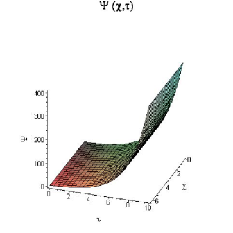
Figure 1: The wave function of the universe is formally defined for the AVTD solution as $|\Psi\rangle_{AVTD}\sim\exp(\lambda_{AVTD}/2)=\exp[(\lambda_{0}+c^{2}\tau)/2]$, according to Eq.(25). The graphic shows the singular behavior of $|\Psi\rangle_{AVTD}$, for $\tau\rightarrow\infty$, with $c=1$, and $\lambda_{0}=1$.

The wave function of the universe for this special case is depicted in Fig. 2, where we can see that it is regular for all values of $\chi$ and $\tau$. As the classical singularity ($\tau\rightarrow\infty$) is approached, the wave function of the universe remains constant and finite. This result shows that the classical cosmological singularity of this particular Gowdy model has been removed after its canonical quantization in the context of $N=1$ supergravity. The presence of the fermionic field is thus sufficient to solve the singularity problem at the quantum level in this particular midisuperspace model. To obtain this result we have considered in (44) only the first two nontrivial terms of an infinite series. If we consider further terms, the expression for the corresponding function $\lambda$ become rather cumbersome and difficult to handle. Nevertheless, since all higher terms contain only Bessel functions, the mathematical structure of the function $\lambda$ resembles that of Eq.(45) so that for further terms we can expect again wave functions of the universe which are free of singularities. To confirm in an invariant way that no singularities appear in the wave function of the universe we have analyzed the curvature spatial scalar $R=e^{\ a}_{\alpha}R^{\alpha}_{\ a}$, which characterizes the structure of the constant time hypersurface where the wave function of the universe is defined. In the present case we find that $R=-(1/2)\exp[(\lambda-\tau)/2]P_{\chi}^{2}$, and a numerical analysis of this scalar shows that it is regular everywhere.

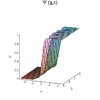
Figure 2: Behavior of the wave function of the universe for the special solution (44), and (45). The AVTD singular behavior for $\tau\rightarrow\infty$, has disappeared and it is replaced by a well-behaved function with a constant value.

Let us now consider the general case in which the components of the wave function depend also on the spatial coordinates $\sigma$ and $\delta$. Using the method of separation of variables, it is easy to show that the general solution to the system (IV.1)-(IV.1) must have the form

$$|\Psi\rangle=\left(\begin{array}[]{c}\Psi_{I}\\ \Psi_{II}\\ \Psi_{III}\\ \Psi_{IV}\end{array}\right)=e^{m\sigma+n\delta+g(\chi)}\left(\begin{array}[]{c}a_{0}\\ b_{0}\\ c_{0}\\ d_{0}\end{array}\right)\,,$$ (46)

where $m$ and $n$ are constants which arise from the separation of variables, and $g(\chi)$ is a function to be determined. Furthermore, $a_{0},\ b_{0},\ c_{0},$ and $d_{0}$ are arbitrary constants. Inserting this ansatz for the wave function into Eqs.(IV.1) and (IV.1), we obtain one single differential equation

$$g_{\chi}=\frac{1}{4}\lambda_{\chi}\mp\frac{i}{4}P_{\chi}+e^{-\frac{1}{4}(\lambda-2P-3\tau)}\left[e^{-P}m\frac{a_{0}+d_{0}}{b_{0}-a_{0}}+n\frac{a_{0}+c_{0}}{b_{0}-a_{0}}\right]\ ,$$ (47)

if the following relationships are satisfied

$$c_{0}(b_{0}-a_{0})+d_{0}(a_{0}+b_{0})=0\ ,\quad d_{0}(a_{0}-b_{0})+c_{0}(a_{0}+b_{0})=0\ .$$ (48)

Similarly, from Eqs.(IV.1) and (IV.1) we obtain

$$g_{\chi}=\frac{1}{4}\lambda_{\chi}\mp\frac{i}{4}P_{\chi}+e^{-\frac{1}{4}(\lambda-2P-3\tau)}\left[e^{-P}m\frac{b_{0}+c_{0}}{c_{0}+d_{0}}-n\frac{a_{0}-c_{0}}{c_{0}+d_{0}}\right]\ ,$$ (49)

when the conditions (48) are fulfilled. Notice that Eqs.(48) imply that $a_{0}^{2}+b_{0}^{2}=0$ and $c_{0}^{2}+d_{0}^{2}=0$ so that we can choose

$$a_{0}=\pm ib_{0}\ ,\qquad c_{0}=\mp id_{0}\ ,$$ (50)

as the general solution for the system (48). Comparing term by term the two equations for the function $g_{\chi}$ given above we find two new conditions on the constants $b_{0}$ and $d_{0}$, i.e.

$$(a_{0}+d_{0})(c_{0}+d_{0})=(b_{0}+c_{0})(b_{0}-a_{0})\ ,\quad(a_{0}+c_{0})(c_{0}+d_{0})=(a_{0}-c_{0})(a_{0}-b_{0})\ .$$ (51)

Notice that these conditions follow from the terms containing the constants “$m$” and “$n$” in Eqs.(47) and (49) so that they are valid only if $m\neq 0$ and $n\neq 0$. It is now easy to see that Eqs.(51) does not allow any solutions compatible with (50). Consequently, the only compatible solution is for $m=0=n$, a result which implies that an explicit dependence on the spatial coordinates $\sigma$ and $\delta$ is not allowed and, therefore, the existence of anomalies in the wave function of the universe is completely excluded.

Under the above considerations, the resulting differential equation for $g(\chi)$ can easily be integrated and yields $g(\chi)=(\lambda\mp iP)/4$. The imaginary part can again be considered as a phase and, therefore, the behavior of the wave function of the universe is completely dictated by the behavior of the metric function $\lambda$ only. The explicit final expression for $|\Psi\rangle$ coincides with the one of the former case given in Eq.(41).

IV.2 The unpolarized case

In this Section we will analyze the general unpolarized $T^{3}$ Gowdy model $(Q\neq 0)$. No general solution to the classical field equations is known in this case because of their highly nonlinear character. In fact, only a few exact highly nontrivial solutions are known in the literature oqr1 ; oqr2 ; nosotros ; procmike . Let an example be given for the functions $P$, $Q$, and $\lambda$ satisfying the field equations (20)– (23). This is all the information we need to know in order to investigate the supersymmetric constraint $S|\Psi\rangle=0$ which yields the following set of equations

$$\partial_{\chi}(\Psi_{I}+\Psi_{II})-\frac{1}{4}(\lambda_{\chi}-P_{\chi})\Psi_{I}-\frac{1}{4}(\lambda_{\chi}+P_{\chi})\Psi_{II}-\frac{1}{2}e^{P}Q_{\chi}\Psi_{III}$$

$$+e^{-\frac{1}{4}(\lambda-2P-3\tau)}\left[e^{-P}\partial_{\sigma}(\Psi_{II}+\Psi_{III})-Q\partial_{\sigma}(\Psi_{II}-\Psi_{IV})+\partial_{\delta}(\Psi_{II}-\Psi_{IV})\right]=0\,,$$ (52)

$$\partial_{\chi}(\Psi_{II}-\Psi_{I})-\frac{1}{4}(\lambda_{\chi}-P_{\chi})\Psi_{II}+\frac{1}{4}(\lambda_{\chi}+P_{\chi})\Psi_{I}+\frac{1}{2}e^{P}Q_{\chi}\Psi_{IV}$$ (53)

$$-e^{-\frac{1}{4}(\lambda-2P-3\tau)}\left[e^{-P}\partial_{\sigma}(\Psi_{I}+\Psi_{IV})-Q\partial_{\sigma}(\Psi_{I}+\Psi_{III})+\partial_{\delta}(\Psi_{I}+\Psi_{III})\right]=0\,,$$

$$\partial_{\chi}(\Psi_{IV}-\Psi_{III})+\frac{1}{4}(\lambda_{\chi}-P_{\chi})\Psi_{III}-\frac{1}{4}(\lambda_{\chi}+P_{\chi})\Psi_{IV}-\frac{1}{2}e^{P}Q_{\chi}\Psi_{I}$$

$$-e^{-\frac{1}{4}(\lambda-2P-3\tau)}\left[e^{-P}\partial_{\sigma}(\Psi_{I}+\Psi_{IV})-Q\partial_{\sigma}(\Psi_{II}+\Psi_{IV})+\partial_{\delta}(\Psi_{II}+\Psi_{IV})\right]=0\,,$$ (54)

$$-\partial_{\chi}(\Psi_{III}+\Psi_{IV})+\frac{1}{4}(\lambda_{\chi}-P_{\chi})\Psi_{IV}+\frac{1}{4}(\lambda_{\chi}+P_{\chi})\Psi_{III}+\frac{1}{2}e^{P}Q_{\chi}\Psi_{II}$$

$$+e^{-\frac{1}{4}(\lambda-2P-3\tau)}\left[e^{-P}\partial_{\sigma}(\Psi_{II}+\Psi_{III})+Q\partial_{\sigma}(\Psi_{I}-\Psi_{III})-\partial_{\delta}(\Psi_{I}-\Psi_{III})\right]=0\,.$$ (55)

It is clear that an exponential ansatz with separation of variables similar to the one used in the previous case in Eq.(46) will lead to a system of ordinary differential equations and a set of algebraic equations. The analysis of the resulting equations is similar to the one performed in the last subsection for the polarized case. In a similar manner, it is possible to show that no anomalies are allowed in the wave function of the universe which therefore turns out to depend on the spatial coordinate $\chi$ only. The resulting wave function of the universe can be expressed as

$$|\Psi\rangle=\left(\begin{array}[]{c}\Psi_{I}\\ \Psi_{II}\\ \Psi_{III}\\ \Psi_{IV}\end{array}\right)=e^{h(\chi)}\left(\begin{array}[]{c}a_{0}\\ b_{0}\\ c_{0}\\ d_{0}\end{array}\right)\,,$$ (56)

where the set of constants must satisfy the conditions

$$c_{0}(b_{0}-a_{0})+d_{0}(a_{0}+b_{0})=0\ ,\quad d_{0}(a_{0}-b_{0})+c_{0}(a_{0}+b_{0})=0\ ,$$ (57)

which allow the solution $a_{0}=\pm ib_{0}$, $c_{0}=\mp id_{0}$. For the sake of simplicity we consider the case in which $b_{0}$ and $d_{0}$ are real constants. Then, the function $h(\chi)$ can be put in the form

$$h(\chi)=\frac{1}{4}\lambda-\frac{d_{0}}{4b_{0}}\int e^{P}Q_{\chi}\,d\chi\mp\frac{i}{4}\left(P+\frac{d_{0}}{b_{0}}\int e^{P}Q_{\chi}\,d\chi\right)\ .$$ (58)

This function together with the conditions (57) represent an explicit solution of the supersymmetric constraint and show that in the unpolarized case there exist nontrivial physical states. The imaginary part of $h(\chi)$ can again be interpreted as a phase which does not affect the behavior of the wave function of the universe (56). The behavior of the real part of $h(\chi)$ is governed by the behavior of the metric function $\lambda$ and an integral which involves the functions $P$ and $Q$. Hence, we need the explicit form of the metric in order to analyze the wave function of the universe. As mentioned before, it is very difficult to solve the system of differential equations which follow from Einstein’s vacuum field equations. To analyze the behavior of the wave function near the singularity it would be necessary to apply numerical methods for handling the metric functions. This is a task which is outside the scope of the present work.

V Final remarks and conclusions

Our analysis of the supersymmetric constraint presented in the last sections relies on a very specific foliation of spacetime. In fact, the general form of the constraint ${\cal S}=\varepsilon^{0\alpha\beta\delta}\gamma_{5}\gamma_{\alpha}D_{\beta}\psi_{\delta}$ fixes at the very beginning the time coordinate $x^{0}$ so that it does not appear as a dynamical variable in the further analysis. Here we have chosen $x^{0}=\tau$ which is the natural time coordinate in Gowdy cosmological models. The canonical quantization formalism forces us to “freeze” this time during the entire analysis and it reappears explicitly only in the solutions for the wave function of the universe, where we interpret it as a label which associates a particular value of the wave function to a different spatial slice. It is in this sense that we can say that we know explicitly the wave function of the universe at each moment of time. And it is in this context that we were able to investigate the behavior of the wave function near the cosmological singularity.

Consequently, the problem of the “frozen” time in our analysis cannot be solved in the context of the canonical quantization formalism. The common concern about the use of this formalism is whether the final result of the quantization (in our case, the wave function of the universe) depends on the choice of a particular foliation. To clarify this question in the present case let us consider a different quite general foliation. Consider a new time coordinate $t$ defined by

$$dt=e^{-\frac{1}{4}(\lambda+3\tau)}d\tau\ .$$ (59)

Then, from the general line element (19) we obtain

$$ds^{2}=dt^{2}-e^{2\Lambda}d\chi^{2}-e^{F}\left(e^{P}d\sigma^{2}+e^{-P}d\delta^{2}\right)\ ,$$ (60)

where $\Lambda=\Lambda(t,\chi)$ and $F=F(t,\chi)$. For the sake of simplicity we are considering here the polarized case only $(Q=0)$. In this particular parametrization the lapse function becomes a constant. We apply now the canonical quantization procedure of supergravity with a foliation determined by $x^{0}=t=$const. Clearly, this is a quite radical change of foliation when compared with the original one $(\tau=$const). To calculate the supersymmetric constraint we proceed as in Section IV for the non-trivial solution (18). Then we obtain

$${\cal S}=e^{\Lambda+2F}{\cal S}_{1}+e^{\frac{1}{2}(4\Lambda+3F+P)}{\cal S}_{2}\ ,$$ (61)

with

$${\cal S}_{1} = \left(\partial_{\chi}+\Lambda_{\chi}+\frac{1}{4}P_{\chi}+\frac{7}{4}F_{\chi}\right)\Gamma^{1}+\left(\partial_{\chi}+\Lambda_{\chi}-\frac{1}{4}P_{\chi}+\frac{7}{4}F_{\chi}\right)\Gamma^{2}\ ,$$ (62)

$${\cal S}_{2} = e^{-P}\Gamma^{4}\partial_{\sigma}-\Gamma^{5}\partial_{\delta}\ \,.$$ (63)

If we compare these expressions with the supersymmetric constraint in the original foliation, given in Eqs.(32) and (33), we see that the general structure does not change. The integration of the differential equations following from applying (62) and (63) to the wave function leads to a solution with a structure similar to that of Eq.(41). This shows that the general behavior of the wave function of the universe is qualitatively invariant with respect to a transformation of the time coordinate as given in Eq.(59). This coordinate transformation of time is quite general since it involves all the nonignorable coordinates present in Gowdy models and implies a constant lapse function. Clearly, the qualitative independence of the wave function of the universe holds also in the case of less general coordinate transformations.

It is necessary to mention that for the expression of the Lorentz constraint in terms of the gravitino field (7) there is only one possible choice, namely

$$\phi_{1}\sim\gamma^{1}\ ,\quad\phi_{2}\sim\gamma^{2}\ ,\quad\phi_{3}\sim\gamma^{3}\ .$$ (64)

On the other hand, for the solution of the supersymmetric constraint we use the choice (34) which is more convenient for the analysis of the resulting differential equations. Nevertheless, one could use the representation (64) since the final result for the wave function of the universe does not depend on the particular used representation.

It is important to emphasize that the physical interpretation of the wave function of the universe $|\Psi\rangle$ presents certain difficulties. A genuine wave function must be related to observable quantities and this implies that $|\Psi\rangle$ must yield a probability density. However, this is not true in this case, in particular because the wave function of the universe is not normalizable. Moreover, if we require that $|\Psi\rangle$ yields a probability density for the 3-geometry which must have a specific value at a given time, this would imply a violation of the Hamiltonian constraint kucryan . These difficulties in the interpretation of the wave function of the universe are the price one has to pay for applying the canonical quantization procedure which involves the isolation of a specific “time” parameter against which the evolution of the system can be defined. An alternative procedure like the Dirac quantization based on functional integrals, which does not require to single out the time variable, could lead to a quantum system with less interpretation difficulties guvryan .

In this work we have investigated the Gowdy $T^{3}$ cosmological models in the context of $N=1$ supergravity. The quantum constraints resulting from the canonical quantization formalism were explicitly analyzed, and for the resulting set of differential equations we were able to find general solutions. In this way, we found the wave function of the universe for the polarized and unpolarized special cases. This represents a proof of the existence of physical states in the $(N=1)$ supersymmetric midisuperspace corresponding to Gowdy cosmologies. This result contrasts drastically with analogous investigations in minisuperspace (Bianchi) models where no physical states exist, a result that sometimes is assumed as a sufficient proof to dismiss supergravity $N=1$. We have adopted a less radical position in this work and dismiss as unphysical only the minisuperspace models. The existence of physical states in midisuperspace models confirms this conclusion and indicates that supergravity $N=1$ is a valuable theory which should be investigated further. In this context we have also obtained an interesting result showing that, in the Gowdy $T^{3}$ midisuperspace model analyzed in this work, the wave function of the universe which represents nontrivial physical states is completely free of anomalies.

Gowdy cosmologies are characterized by the existence of a curvature singularity at temporal infinity, and it is known that the metric functions near the singularity evolve according to the AVTD behavior. We have shown that after the canonical quantization the corresponding wave function of the universe is free of singularities. This represents a solution to the singularity problem and is one of the main results of this work. The mere presence of the Rarita-Schwinger field and the consideration of a genuine midisuperspace model is sufficient to eliminate the classical singularity. This result points to a further interesting and expected property of supergravity $N=1$ in the sense that it is able to properly handle the conceptual limits of classical general relativity.

In this work we focused on the special case of $T^{3}$ cosmologies. The generalization of our results to include the case of $S^{1}\times S^{2}$ Gowdy models seems to be straightforward. In particular, we believe that the unified parametrization introduced in procmike , which contains both types of topologies, could be useful to explore the supersymmetric Gowdy model in quite general terms.

- (1) P. van Nieuwenhuizen, Phys. Rept. 68 189 (1981); S. Ferrara (ed.), Supersymmetry, Vol. 1 & 2 (World Scientific, Singapore, 1989); A. Salam and E. Sezgin (eds.), Supergravities in diverse dimensions, Vol. 1 & 2 (World Scientific, Singapore, 1989).
- (2) M. Green, J. Schwarz and E. Witten, Superstring theory, Vol. 1 & 2 (Cambridge University Press, Cambridge, England, 1987); D. Lüst and S. Theisen, Lectures on string theory, (Springer Verlag, Berlin, 1989); J. Polchinski, String theory, Vol. I & II (Cambridge University Press, Cambridge, England, 1998); E. Kiritsis, Introduction to superstring theory, Leuven notes in mathematics and theoretical physics, 9 (1997), hep-th/9709062.
- (3) M. Pilati, Nucl. Phys. B132 138 (1978).
- (4) C. Teitelboim, Phys. Lett. B69 240 (1977); Phys. Rev. Lett. 38 1106 (1977); R. Tabensky and C. Teitelboim, Phys. Lett. B69 453 (1977).
- (5) P.D. D’Eath, S. Hawking, and O. Obregón, Phys. Lett. B300 44 (1993).
- (6) R. Graham and A. Csordás, Phys. Rev. Lett. 74 4129 (1995).
- (7) A. Csordás and R. Graham, Phys. Lett. B373 51 (1996).
- (8) P.D. D’Eath, Phys. Rev. D29 2199 (1984). Phys. Lett. B321 368 (1994).
- (9) O. Obregón, J. Pullin, and M.P. Ryan, Phys. Rev. D48 5642 (1993).
- (10) A. Macías, O. Obregón and J. Socorro, Int. J. Mod. Phys. A8 4291 (1993).
- (11) A. Macías, E.W. Mielke, and J. Socorro, Int. J. Mod. Phys. D7 701 (1998).
- (12) A. Macías, Gen. Rel. Grav. 31 653 (1999).
- (13) B. S. DeWitt, Phys. Rev. 160 1113 (1967); C. W. Misner, Phys. Rev. 186 1319 (1969).
- (14) M.P. Ryan: Hamiltonian Cosmology (Springer, New York, 1972). M.P. Ryan and L.C. Shepley: Homogeneous Relativistic Cosmologies (Princeton University Press, New Jersey, 1975).
- (15) K. V. Kuchar and M. P. Ryan, Phys. Rev. D 40 3982 (1989).
- (16) J. B. Hartle and S. W. Hawking, Phys. Rev. D12, 2960 (1983).
- (17) A. Vilenkin, Phys. Rev. D30 509 (1984).
- (18) D. Kramer, D. Stephani, E. Herlt, M. MacCallum, and E. Schmutzer, Exact Solutions of Einstein’s Field Equations (Cambridge University Press, Cambridge, England, 1980).
- (19) R. Gowdy, Phys. Rev. Lett. 27 826 (1971).
- (20) R. Gowdy, Ann. Phys. (N. Y.) 83 203 (1974).
- (21) B. Berger, Liv. Rev. Rel. 5 1 (2002).
- (22) A. Macías, E.W. Mielke, and J. Socorro, Phys. Rev. D57 1027 (1998).
- (23) A. Macías, O. Obregón and M. P. Ryan, Class. Quantum Grav. 4 1477 (1987).
- (24) M. Kaku: Quantum Field Theory (Oxford University Press 1993).
- (25) P. van Nieuwenhuizen, Phys. Rep. 68 189 (1981).
- (26) A. Asthekar and M. Pierri, J. Math. Phys. 37 6250 (1996).
- (27) A. Corichi, J. Cortez, and H. Quevedo, Int. J. Mod. Phys. D11 1451 (2002).
- (28) V. Moncrief, Ann. Phys. (N. Y.) 132 87 (1981); J. Isenberg and V. Moncrief, Ann. Phys. (N.Y.) 199 84 (1990); P. T. Crusciel, J. Isenberg and V. Moncrief, Class. Quantum Grav. 7 1671 (1990); B. Grubisic and V. Moncrief, Phys. Rev. D47 2371 (1993); B.K. Berger and V. Moncrief, Phys. Rev. D48 4676 (1993); D. Garfinkle, Phys. Rev. D60 104010 (1999); T. Jurke, Class. Quantum Grav. 20 173 (2003); M. Chae and P. T. Chrusciel, gr-qc/0305029; P. T. Chrusciel and K. Lake, Class. Quantun Grav. 21, S153 (2004); L. Andersson, H. van Elst, and C. Uggla, Class. Quantun Grav. 21 S29 (2004).
- (29) O. Obregon, H. Quevedo, and M. P. Ryan, Phys. Rev. D65 024022 (2002).
- (30) O. Obregon, H. Quevedo, and M. P. Ryan, Phys. Rev. D70 064035 (2004).
- (31) A. Sánchez, A. Macías and H. Quevedo, J. Math. Phys. 45 1849 (2004).
- (32) B. K. Berger and D. Garfinkle, Phys Rev. D57 4767 (1998); D. Garflinke and M. Weaver, Phys. Rev. D67 124009 (2003).
- (33) J. Isenberg and V. Moncrief, Ann. Phys. (N.Y.) 199 84 (1990); P. T. Crusciel, J. Isenberg and V. Moncrief, Class. Quantum Grav. 7 1671 (1990); B. K. Berger, Ann. Phys. (N.Y.) 83 458 (1974); B. Grubisic and V. Moncrief, Phys. Rev. D47 2371 (1993).
- (34) H. Quevedo, in: Exact solutions and scalar fields in gravity: Recent results. A. Macías, J. Cervantes-Cota and C. Lämmerzahl (Eds.) (Kluwer Press, New York, 2001).
- (35) D. Eardley, E. Liang and R. Sachs, J. Math. Phys. 13 99 (1972).
- (36) S.M. Carroll, D. Z. Freedman, M.E. Ortiz, and D. Page, Nucl. Phys. B423 661 (1994).
- (37) H. Quevedo, Gen. Rel. Grav. (2005), in press, gr-qc/0409051.
- (38) J. Guven and M. P. Ryan, Phys. Rev. D45 3559 (1992).