de Sitter and double irregular domain walls

Abstract

A new method to obtain thick domain wall solutions to the coupled Einstein scalar field system is presented. The procedure allows the construction of irregular walls from well known ones, such that the spacetime associated to them are physically different. As consequence of the approach, we obtain two irregular geometries corresponding to thick domain walls with $dS$ expansion and topological double kink embedded in $AdS$ spacetime. In particular, the double brane can be derived from a fake superpotential.

KEY WORDS: thick branes, de Sitter walls, BPS walls

1 Introduction

The gravitational properties of domain walls or 3-branes have been object of intense investigation for different reasons. On one hand, it has been pointed out that four-dimensional gravity can be realized on a thin wall interpolating between Anti-de Sitter ($AdS$) spacetimes [1, 2, 3]. On the other hand, wall configurations are relevant for the study of Renormalization-Group flow Equations in the context of Anti-de Sitter/Conformal Field Theory correspondence [4].

Considering our four-dimensional universe as an infinitely thin domain wall is an idealization, and it is for this reason, that in more realistic models the thickness of the brane has been taken into account [5, 6, 7, 8, 9, 10, 11, 12]. The thick domain walls are solutions to Einstein’s gravity theory interacting with a scalar field, where the scalar field is a standard topological kink interpolating between the minima of a potential with spontaneously broken symmetry. The nonlinearity of the five-dimensional Einstein’s gravity theory interacting with a scalar field represents a strong difficulty when finding exact solutions to the system. In this sense, several formulations and methodologies [13, 5, 14, 15, 16] have been reported, where it is possible to reconsider the problem in a simpler way. Maintaining this focus, in this paper, we develop a new formulation or method based on the linearization of one of the equations of the system.

We show that the coupled system with planar symmetry, admits two solutions, physically not equivalent, associated to a scalar field, with different self-interaction potentials. We have called these solutions regular and irregular solutions, because in the last case the geometry spacetime hosts a coordinate singularity defined by a hypersuperface of codimension one. In [17] we made simultaneous use of the regular and irregular solutions and showed that it is possible to generate asymmetric brane worlds with interesting properties, where the irregular contribution plays an important role on the asymmetry in the brane. In this sense, in the present paper, we analyze the explicit realization of the domain walls on those irregular spacetimes.

In section III, we consider a regular brane with a de Sitter ($dS$) expansion [18] and we find that the irregular geometry corresponds to a domain wall with similar features interpolating between two $AdS$ vacua. It is well known that due to the non-linearity and instability of the gravitational interactions, the inclusion of the gravitational evolution into a dynamic thick wall is a highly non-trivial problem. For this reason, there are not so many analytic solutions of a dynamic thick domain wall. In fact, to our knowledge, in the literature encountered so far, there only exist two solutions [18, 19], with background metric on the brane given by a $dS$ expansion, which resembles the Friedmann-Robertson-Walker metric, typical in a cosmological framework.

In section IV, we obtain an irregular topological double kink geometry embedded into an $AdS$ background, from the double regular configuration analyzed in [16], and show that this irregular spacetime is derivable from a fake superpotential. In the context of static domain wall spacetime, the double walls are topological defects richer than the standard topological kinks. These configurations may be seen as defects that host internal structure, representing two parallel walls, whose properties have been studied in several papers: in [20], using models described by a complex scalar field; in [21, 22, 23], in models described by two real scalar fields on flat spacetime; and in [24], in brane scenarios involving two higher dimensions on curved spacetime. On the other hand, the models supported on a single real scalar field, with a $2$-kink profile have only been considered in [16, 25], thus the irregular double domain wall considered here, corresponds to another example of these exotic configurations.

Finally, in section V we summarize our results.

2 Approach to generate new solutions

Consider the action of Einstein’s gravity theory interacting with a real scalar field $\phi$

$$S=\int d^{4}ydx\sqrt{-\mathrm{g}}\left[\frac{1}{2}R-\frac{1}{2}\mathrm{g}^{\mu\nu}\nabla_{\mu}\phi\nabla_{\nu}\phi-V(\phi)\right],$$ (1)

where $\mathrm{g}$ is the metric tensor, $R$ is the scalar curvature and $V(\phi)$ the scalar potential. The field equations generated from last action has the form

$$G_{ab}=R_{ab}-\frac{1}{2}\ \mathrm{g}_{ab}\ R=T_{ab},$$ (2)

$$T_{ab}=\nabla_{a}\phi\ \nabla_{b}\phi-\mathrm{g}_{ab}\left[\frac{1}{2}\ \nabla^{c}\phi\ \nabla_{c}\phi+V(\phi)\right],$$ (3)

$$\nabla^{c}\nabla_{c}\phi-\frac{dV(\phi)}{d\phi}=0,$$ (4)

with $G_{ab}$ the Einstein tensor, $R_{ab}$ the Ricci tensor and $T_{ab}$ the stress-energy tensor.

Let $\mathrm{g}$ be the metric tensor for a 5-dimensional spacetime with planar-paralell symmetry, given by [26]

$$\mathrm{g}_{ab}=f(x)^{2}\ \left(-dt_{a}\ dt_{b}+e^{2\beta t}\ dy_{a}^{j}\ dy_{b}^{j}\right)+f(x)^{2}\ dx_{a}\ dx_{b},\quad\beta>0,$$ (5)

where $\ j=1,2,3\$ and $a,\ b=0,\dots,4$. We look for solutions to the coupled Einstein-scalar field system (2-4) satisfying the requirements

1.-

$\ \phi=\phi(x)$,

2.-

$\lim_{x\rightarrow\pm\infty}\phi(x)=\varphi_{\pm}$   such that   $\lim_{\phi\rightarrow\varphi_{\pm}}\frac{dV(\phi)}{d\phi}=0$,    $\varphi_{\pm}\in\Re$

3.-

$\ \phi^{\prime}(x)^{2}$ is symmetric under reflections in the $x=0$ plane,

where the prime denotes derivative with respect to $\ x$. Following the usual strategy, we find

$$\phi^{\prime}(x)^{2} = f^{2}\ \left(G_{4}{}^{4}-G_{0}{}^{0}\right)=6\ \frac{f^{\prime\ 2}}{f^{2}}-3\ \frac{f^{\prime\prime}}{f}-3\ \beta^{2}\ ,$$ (6)

$$V(\phi(x)) = -\frac{1}{2}\ \left(G_{4}{}^{4}+G_{0}{}^{0}\right)=-3\ \frac{f^{\prime\ 2}}{f^{4}}-\frac{3}{2}\ \frac{f^{\prime\prime}}{f^{3}}+\frac{9}{2}\frac{1}{f^{2}}\ \beta^{2}.$$ (7)

Now, if we rewrite (6) in terms of the inverse function of the metric factor, i.e. $g=1/f$, we obtain

$$g^{\prime\prime}(x)-\left[\frac{1}{3}\ \phi^{\prime}(x)^{2}+\beta^{2}\right]\ g(x)=0.$$ (8)

This equation is the Sturm-Liouville type and it is well known that has an orthogonal set of solutions $\ \{g_{1},\ g_{2}\}\$ associated, where

$$g_{2}(x)=g_{1}(x)\ \chi(x);\qquad\chi(x)\equiv\int_{x_{0}}^{x}\ \frac{1}{g_{1}(\xi)^{2}}\ d\xi$$ (9)

and the general solution

$$g(x)=g_{1}(x)\left(c_{1}+c_{2}\ \chi(x)\right),\qquad c_{1},\ c_{2}\in\Re$$ (10)

depends on two arbitrary constans.

Remarkably enough, equation (9) gives a mechanism to obtain new solutions to the coupled system from known ones, such as $g_{1}$, compatible with the same scalar field but with different potentials. We are interested in the realization of domain walls on the geometry defined by $g$, in such sense we will consider $g_{1}$ as functions whose analytic behavior generate new domain wall solutions to (2-4).

Let $\ g_{1}\$ be a function such that

1.-

$\ g_{1}\$ is $C^{2}$,

2.-

$\ g_{1}\ >\ 0$ (positive definite),

3.-

$\ g_{1}\$ is a function asymptotically increasing,

then $f_{1}$ is a continuous, integrable and asymptotically vanishing function, which we will call regular; and $g$ is smooth function with a zero in some value of $x$, corresponding to a singularity in $f$, for the following cases

1.-

If $c_{1},c_{2}\neq 0$, then $g$ will have a zero in $x_{p}\in x$ when $\chi(x)|_{x_{p}}=-c_{1}/c_{2}.$

2.-

If $c_{1}=0$ and $c_{2}\neq 0$, then $g$ will have a zero in $x_{0}$.

In the first case, it is possible to avoid the divergence in (5). It is only necessary to choose appropriately the constants $c_{1}$ and $c_{2}$, so that its negative quotient does not belong to the image of $\chi(x)$. In the ref. [17], we developed and discussed this kind of solutions for two exotic branes and show that it is possible to localize the four-gravity on them. In the second case the divergence in (5) is unavoidable, however in this paper we explore the possibility to set up domain walls on this geometry, where the metric factor is singular or irregular.

To study the above irregular solutions further, let us first note that all the scalars built from the Riemann tensor are finite in the whole bulk. Thus, the spacetime described by the irregular solutions are free of scalar singularities. Moreover, for the hypersurfaces $\ x=x_{0}$, the tidal forces experimented by a freely falling observer become bounded. To show this explicitly, let us consider the nonvanishing components of the Riemann curvature tensor with respect to the static orthonormal frame $R_{0j0j}=-R_{1k1k}=-R_{2323}$, $R_{j4j4}=-R_{0404}$ where $j=1,2,3;\ k=2,3$ and

$$R_{2323}=\beta^{2}\ g^{2}-g^{\prime 2}\ ,\qquad R_{0404}=g^{\prime 2}-g\ g^{\prime\prime}\ .$$ (11)

Free falling observers with energy $E$ are connected to the static orthonormal frame by a local Lorentz boost in the direction perpendicular to the wall, with an instantaneous velocity given by

$$v^{\hat{4}}=\sqrt{1-E^{-2}\ g^{-2}}\ .$$ (12)

Then the nonvanishing curvature components in the Lorentz boosted frame are $R_{\hat{k}\hat{4}\hat{k}\hat{4}}$, $R_{\hat{2}\hat{3}\hat{2}\hat{3}}$, $R_{\hat{0}\hat{k}\hat{0}\hat{k}}$, $R_{\hat{0}\hat{4}\hat{0}\hat{4}}$, $R_{\hat{0}\hat{k}\hat{k}\hat{4}}=R_{\hat{k}\hat{4}\hat{0}\hat{k}}$ where $\hat{k}=\hat{2},\hat{3}$ and

$$R_{\hat{k}\hat{4}\hat{k}\hat{4}}=-E^{2}\ g^{3}\ (\beta^{2}\ g-g^{\prime\prime})-g^{\prime 2},\qquad\qquad\quad$$ (13)

$$R_{\hat{0}\hat{k}\hat{0}\hat{k}}=-E^{2}\ g^{3}\ (\beta^{2}\ g-g^{\prime\prime})+g^{\prime 2}-g\ g^{\prime\prime},$$ (14)

$$R_{\hat{0}\hat{k}\hat{k}\hat{4}}=-E\ g\ \sqrt{E^{2}\ g^{2}-1}\ (\beta\ g-g^{\prime\prime}),$$ (15)

$$R_{\hat{2}\hat{3}\hat{2}\hat{3}}=\beta^{2}\ g^{2}-g^{\prime 2},$$ (16)

$$R_{\hat{0}\hat{4}\hat{0}\hat{4}}=g^{\prime 2}-g\ g^{\prime\prime}$$ (17)

According to equations (13-17), none of the components of Riemann in the explorer’s orthonormal frame become infinite in the pathological point $x=x_{0}$. Therefore, the metric $\mathrm{g}$ on the surface $x=x_{0}$ is a nonsingular and perfectly well-behaved region of spacetime. We think that there must be a differentiable chart for which the resulting differentiable structure gives a smooth metric, but to find these coordinates is not the purpose of this paper.

As a final comment, it is important to remark that geometries obtained from $g_{1}$ and $g$ with metric tensors $\mathrm{g}_{1\mu\nu}$ and $\mathrm{g}_{\mu\nu}$ are physically different, because it does not exist a diffeomorphism among them. In fact, the spacetimes are connected by a conformal transformation given by

$$\mathrm{g}_{1\mu\nu}=\Omega^{2}\mathrm{g}_{\mu\nu},\qquad\Omega\equiv c_{1}+c_{2}\chi(x).$$ (18)

In concordance with [28], the conformal transformations should not be understood as diffeomorphisms, but as applications that allow to connect two different spacetimes with identical causal structure. In this sense, we can conclude that the manifolds with metric tensors $\mathrm{g}_{1\mu\nu}$ and $\mathrm{g}_{\mu\nu}$ are physically not equivalent.

3 Irregular domain wall with a de Sitter expansion

Consider the embedding of a thick $dS$ 3-brane into a five-dimensional bulk described by the metric (5), with a reciprocal metric factor given by

$$g_{1}(x)=\cosh^{\delta}\left(\beta x/\delta\right),\quad 1/2>\delta>0,\quad\beta>0,$$ (19)

In Ref. [18, 30], it has been shown that this spacetime is a solution to the coupled Einstein-scalar field equations with

$$\phi=\phi_{0}\arctan\left(\sinh\ \beta x/\delta\right),\qquad\phi_{0}=\sqrt{3\delta(1-\delta)},$$ (20)

and

$$V_{1}(\phi)=\frac{1+3\delta}{2\delta}\ 3\beta^{2}\left(\cos\phi/\phi_{0}\right)^{2(1-\delta)}.$$ (21)

The scalar field takes values $\ \pm\ \phi_{0}\ \pi/2\$ at $\ x\rightarrow\pm\ \infty$, corresponding to two consecutive minima of the potential with cosmological constant $\ \Lambda=0$, and interpolates smoothly between these values at the origin; with $\ \delta\$ playing the role of the wall’s thickness. In [31] it has been shown that this domain wall geometry localizes gravity on the wall, and in [14] that it has a well-defined distributional thin wall limit. We wish to find another thick domain with $dS$ expansion in five-dimensions. From equation (10), choosing $c_{1}=0$ and $c_{2}=1$, with $\ g_{1}\$ given by (19); we obtain

$$g=\frac{i\ \delta}{\beta-2\beta\delta}\ \cosh^{(1-\delta)}(\beta x/\delta)\ \csc\text{h}(\beta x/\delta)\ |\sinh\beta x/\delta|$$ (22)

$${}_{2}F_{1}[l,k,n,\cosh^{2}(\beta x/\delta)],\qquad 1/2>\delta>0,\quad\beta>0,$$ (23)

where ${}_{2}F_{1}$ is the hypergeometric function with $l=1/2-\delta,\ k=l+\delta$, and $n=l+1$. This solution represents a two-parameter family. Then, for simplicity we will consider the case $\delta=1/4$ without loss of generality

$$g(x)=-\frac{i}{2\ \beta}\ \cosh(2\ \beta x)^{1/4}\ F[2i\ \beta x,\>\sqrt{2}],\qquad\beta>0,$$ (24)

where $F$ is the incomplete first order elliptic function [29]. This spacetime is solution to (4) with

$$\phi=\phi_{0}\arctan\left(\sinh\ 4\beta x\right),\qquad\phi_{0}=3/4,$$ (25)

and

$$V(\phi) = -6|\cos\ 4\phi/3|^{1/2}$$ (26)

$$-\frac{21}{8}|\cos 4\phi/3|^{3/2}F[i/2\arg\sinh\tan\ 4\phi/3,2]^{2}$$

$$+|\cos\ 4\phi/3|\ \tan(4\phi/3)F[i/2\ \arg\sinh\tan\ 4\phi/3,\>2],$$

where $\ \phi\$ interpolates smoothly between the two degenerate minima of $\ V(\phi)$, $\ \pm\ \phi_{0}\ \pi/2$. To this spacetime corresponds the following energy density and pressure density

$$\rho(x) = -\frac{3}{4}\ \cosh(4\ \beta x)^{-3/2}\left(8\ \cosh(4\ \beta x)+5\ F[2i\ \beta x,\>2]^{2}\right)$$ (27)

$$+6i\ \tanh(4\ \beta x)\ F[2i\ \beta x,\>2],$$

$$p(x) = -\frac{3}{2}\ \cosh(4\ \beta x)^{-3/2}\left(4\ \cosh(4\ \beta x)+\ F[2i\ \beta x,\>2]^{2}\right)$$ (28)

$$+6i\ \tanh(4\ \beta x)\ F[2i\ \beta x,\>2].$$

Notice that (24) has a zero in $\ x=0$. Hence, the spacetime with tensor metric (5, 24) hosts a singularity defined by a hypersurface of codimension one. However, the solution (24, 25, 26) represents a one-parameter family of plane symmetric irregular domain walls with a $dS$ expansion and reflection symmetry along the direction perpendicular to the walls, being asymptotically $AdS_{5}$ with a cosmological constant $\ \Lambda=-6\ \varepsilon$, where $\varepsilon$ is the bound of Image$\{\chi(x)\}=\{-\varepsilon/2\beta,\ +\varepsilon/2\beta\}$ and for $\ \delta=1/4$, $\ \varepsilon=1.31103\$.

In the Fig. 1, we plot the scalar potential $\ V(\phi)$, the energy density $\ \rho(x)$ and the pressure density $\ p(x)$ associated to this system. In spite of the singularity in (5, 24), we see that $V(\phi)$ is a smooth potential with spontaneously broken symmetry and the energy and pressure density correspond to a thick domain wall embedded in $AdS_{5}$ spacetime.

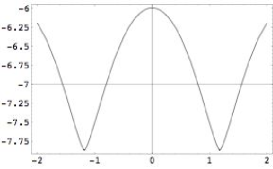
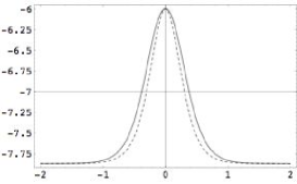
Figure 1: Plots of the new scalar potential $V(\phi)$ for $\delta=1/4$ and $\beta=1$ (left). We also plot (right) the corresponding energy density $\rho(x)$ (continuous line) and pressure $p(x)$ (dotted line), for same values of $\delta$ and $\beta$.

Remarkably, the scalar potential is different in the regular and irregular case. Thus, we have found two domain wall spacetimes with $dS$ expansion compatible with the same scalar field. In [17], we showed that (10), with $g_{1}$ and $g_{2}$ given by (19, 24) respectively, defines another domain wall with interesting properties where it is possible to confine gravity.

4 Irregular double BPS domain walls

Let us now consider a symmetric thick domain wall spacetime where the tensor metric is (5) for $\beta=0$, with

$$g_{1}(x)=\left[1+(\lambda\>x)^{2s}\right]^{1/2s},$$ (29)

where $\lambda\$ and $\ s\$ are real constants with $\ s\$ an odd integer. This solution was presented and broadly discussed in [16, 35] and represents a two-parameter family of plane symmetric static double domain wall, being asymptotically $AdS_{5}$ with a cosmological constant $-6\ \lambda^{2}$.

The metric with reciprocal metric factor (29) is a solution to the coupled Einstein-scalar field equations (2-4) with

$$\phi=\phi_{0}\arctan(\lambda^{s}\>x^{s}),\qquad\phi_{0}=\frac{\sqrt{3(2s-1)}}{s},$$ (30)

and

$$V_{1}(\phi) = \frac{3}{2}\ \lambda^{2}\left[\tan(\phi/\phi_{0})\right]^{2(1-1/s)}$$ (31)

$$\left[\cos(\phi/\phi_{0})\right]^{2(2-1/s)}\left[-1+2s-4\tan^{2}(\phi/\phi_{0})\right],$$

where $\phi$ interpolates between two degenerate minima of $V(\phi)$, $\ \phi(\pm\infty)=\pm\ \phi_{0}\pi/2$. Similar solutions are also considered in [25].

To our knowledge, there are few analytic solutions that host a topological double kink configuration described by a single real scalar field [16, 25]. In this sense, we want to obtain another double domain wall using the method presented in section II. In concordance with our approach, consider (10) with $g_{1}$ given by (29)

$$g=\lambda\>x\>\left[1+(\lambda\>x)^{2s}\right]^{1/2s}{}_{2}F_{1}[l,k,n,-(\lambda\>x)^{2s}],$$ (32)

where $\ l=1/(2s),\ k=2l\$ and $\ n=1+l$. This spacetime is also solution to the coupled system with the scalar field (30) and

$$V(\phi) = -12\lambda^{2}\sin^{2}(\phi/\phi_{0})\>{}_{2}F_{1}[l,k,n;-\tan^{2}(\phi/\phi_{0})]-6\lambda^{2}\cos^{2/s}(\phi/\phi_{0})$$ (33)

$$-\frac{3}{8}\lambda^{2}\sin^{2}(2\phi/\phi_{0})\cos^{-2/s}(\phi/\phi_{0})\>{}_{2}F_{1}[l,k,n;-\tan^{2}(\phi/\phi_{0})]^{2}$$

$$\left[1-2s+4\tan^{2}(\phi/\phi_{0})\right],$$

where $\ \phi\$ takes values $\ \pm\ \phi_{0}\ \pi/2$ at $\ x\rightarrow\pm\infty$, corresponding to two minima of the potential, and interpolates smoothly between them. On the other hand, the energy density of the configuration is given by

$$\rho(x) = -6\lambda^{2}[1+(\lambda\>x)^{2s}]^{-1/s}$$ (34)

$$-12\lambda^{2}(\lambda\>x)^{2s}[1+(\lambda\>x)^{2s}]^{-1}\>{}_{2}F_{1}[l,k,n,-(\lambda\>x)^{2s}]$$

$$-3\lambda^{2}(\lambda\>x)^{2s}[1+(\lambda\>x)^{2s}]^{-2+1/s}[1-2s+(\lambda\>x)^{2s}]$$

$${}_{2}F_{1}[l,k,n,-(\lambda\>x)^{2s}]^{2}.$$

It should be noted that the metric tensor (5, 32) is a singular tensor across of the hypersurface $\ x=0$. However, this is a two-parameter family of plane symmetric static double domain wall spacetime with reflection symmetry along the direction perpendicular to the wall associated to a scalar potential with spontaneously broken symmetry. These walls interpolate between $AdS_{5}$ asymptotic vacua with cosmological constant $\ -6\lambda^{2}[\ \Gamma(l)\Gamma(n)\ ]^{2}/\Gamma(k)^{2}\$. In Fig.2 we plot the potential $\ V(\phi)\$, and the energy density $\ \rho(x)\$ for different values of $\ s$.

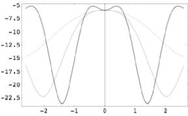
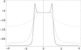
Figure 2: Graphics of the potential $V(\phi)$ (left) and energy density $\rho(x)$ (right) for $s=1,3$ and $7$. The thickness of the lines increases with increasing s.

The energy density shows that the matter field gives rise to thick brane composed of a single ($s=1$) or two ($s\neq 1$) interfaces. In the last case, one sees the appearance of a new phase in between the two interfaces where the energy density of the matter field gets more concentrated. As consequence, a different chart may exist where the metric factor is essentially constant inside the brane [16, 25]; but this is of no concern to us here.

Notice that the potential associated to the irregular case is notably different from the regular case. Thus, we found two solutions to (2-4) compatible with the scalar field (30), but embedded in different $AdS$ backgrounds. In the Ref. [17], we considered the regular and irregular solutions (29, 32) in order to construct an asymmetric brane world with two different walls, where the zero mode of the metric fluctuations is localized on one of them.

Before finishing, we would like to explore the stability of the vacuum. As stated above, the irregular domain wall spacetime considered in this section is asymptotically $AdS_{5}$. It is widely known that $AdS$ vacuum stability requires $V(\phi)$ to take the form [37, 36]

$$V(\phi)=\frac{9}{2}\left(\frac{dW}{d\phi}\right)^{2}-6W^{2},$$ (35)

where $\ W(\phi)$ is any function with at least one critical point, called fake superpotential [38]. Critical points of $\ W(\phi)$ are also critical points of $V(\phi)$ and in the context of supergravity theories the critical points of $\ W(\phi)$ yield stable $AdS$ vacua [37].

It follows that in this case

$$W(\phi) =\lambda\ |\cos^{1/s}(\phi/\phi_{0})|$$ (36)

$$\left[1+\sin^{2}(\phi/\phi_{0})\cos^{-2/s}(\phi/\phi_{0}){}_{2}F_{1}[l,k,n;-\tan^{2}(\phi/\phi_{0})]\right],$$

whose critical points are the asymptotic values of the scalar field, $\ \phi=\pm\pi\phi_{0}/2$. Whether a supergravity theory can be constructed so that the supersymmetry conditions lead to (36) is a question beyond the scope of this paper. But since the critical points of (36) are asymptotic values of $\phi$, as given by (33), this suggests that these asymptotic $AdS$ vacua are stable.

Finally, it should be note that (5, 32) and (30, 33) can be parametrized by (36), so we could have found it using the first order formalism of [39, 13, 5], which in the particular coordinate system (5) is given by

$$g^{\prime}=W(\phi),\qquad g\phi^{\prime}=3\frac{dW(\phi)}{d\phi}.$$ (37)

The domain walls obtained from (35, 37), where the $AdS$ vacua are stable, are solutions that satisfy the Bogomol’nyi-Prasad-Sommerfield (BPS) bound [40, 41, 13]. In this sense, the static double configuration is a BPS domain wall scenario.

5 Summary and Remarks

In this paper we presented a new formulation or method based on the linearization of one of the equations of the coupled Einstein-scalar field system, which gives a mechanism to obtain new solutions from well known ones. We showed that the geometries associated to these solutions are connected by a conformal transformation and, in concordance with [28], the corresponding spacetimes are physically different.

From the approach, we found two thick branes embedded in a spacetime with a nonconventional geometry. These branes correspond to domain walls on a topological space $(\mathbb{R}^{5},\ {\bf g})$, which fails to Hausdorff at the origin and turns out to be singular. However, the components of Riemann tensor in the explorer’s orthonormal frame become bounded in the pathological point. Thus, we conclude that spacetime geometry has a coordinate singularity and the hypersurface hosted at the origin is a well-behaved region of spacetime.

The branes obtained in this paper are explicit realizations of thick domain wall spacetimes. One of them is a $dS$ expansion and the other one is a static topological double kink; both being asymptotically $AdS_{5}$ with $Z_{2}$ symmetry along the direction perpendicular to the wall. These scenarios are the irregular versions of the domain walls reported in [18, 16] and we have considered them in [17] in order to construct exotic brane worlds.

In particular, for the static case, it has been shown that the scalar field potential for this solution satisfies the requirements for the existence of stable $AdS$ vacua, being derivable from a fake superpotential function whose critical points are the asymptotic values of the scalar field. Moreover, this solution can be obtained from the first order formulation of the equations of motion that saturate the BPS bound. Thus, the family of irregular static topological double kink defines a BPS domain wall spacetime.

References

- [1] L. Randall and R. Sundrum, Phys. Rev. Lett. 83, 3370 (1999) [arXiv:hep-ph/9905221].
- [2] L. Randall and R. Sundrum, Phys. Rev. Lett. 83, 4690 (1999) [arXiv:hep-th/9906064].
- [3] M. Cvetic, S. Griffies and H. H. Soleng, Phys. Rev. D 48, 2613 (1993) [arXiv:gr-qc/9306005].
- [4] J. M. Maldacena, Adv. Theor. Math. Phys. 2, 231 (1998) [Int. J. Theor. Phys. 38, 1113 (1999)] [arXiv:hep-th/9711200].
- [5] O. DeWolfe, D. Z. Freedman, S. S. Gubser and A. Karch, Phys. Rev. D 62, 046008 (2000) [arXiv:hep-th/9909134].
- [6] M. Gremm, Phys. Lett. B 478, 434 (2000) [arXiv:hep-th/9912060].
- [7] C. Csaki, J. Erlich, T. J. Hollowood and Y. Shirman, Nucl. Phys. B 581, 309 (2000) [arXiv:hep-th/0001033].
- [8] A. Kehagias and K. Tamvakis, Phys. Lett. B 504, 38 (2001) [arXiv:hep-th/0010112].
- [9] A. Kehagias and K. Tamvakis, Mod. Phys. Lett. A 17, 1767 (2002) [arXiv:hep-th/0011006].
- [10] K. Behrndt and G. Dall’Agata, Nucl. Phys. B 627, 357 (2002) [arXiv:hep-th/0112136].
- [11] S. Kobayashi, K. Koyama and J. Soda, Phys. Rev. D 65, 064014 (2002) [arXiv:hep-th/0107025].
- [12] A. Campos, Phys. Rev. Lett. 88, 141602 (2002) [arXiv:hep-th/0111207].
- [13] K. Skenderis and P. K. Townsend, Phys. Lett. B 468, 46 (1999) [arXiv:hep-th/9909070].
- [14] R. Guerrero, A. Melfo and N. Pantoja, Phys. Rev. D 65, 125010 (2002) [arXiv:gr-qc/0202011].
- [15] D. Bazeia, L. Losano and J. M. C. Malbouisson, Phys. Rev. D 66, 101701 (2002) [arXiv:hep-th/0209027].
- [16] A. Melfo, N. Pantoja and A. Skirzewski, Phys. Rev. D 67, 105003 (2003) [arXiv:gr-qc/0211081].
- [17] R. Guerrero, R. O. Rodriguez and R. Torrealba, Phys. Rev. D 72, 124012 (2005) [arXiv:hep-th/0510023].
- [18] G. Goetz, J. Math. Phys. 31 2683 (1990).
- [19] N. Sasakura, JHEP 0202, 026 (2002) [arXiv:hep-th/0201130].
- [20] A. Campos, K. Holland and U. J. Wiese, Phys. Rev. Lett. 81, 2420 (1998) [arXiv:hep-th/9805086].
- [21] J. R. Morris, Phys. Rev. D 51, 697 (1995).
- [22] D. Bazeia, R. F. Ribeiro and M. M. Santos, Phys. Rev. D 54, 1852 (1996).
- [23] J. D. Edelstein, M. L. Trobo, F. A. Brito and D. Bazeia, Phys. Rev. D 57, 7561 (1998) [arXiv:hep-th/9707016].
- [24] R. Gregory and A. Padilla, Phys. Rev. D 65, 084013 (2002) [arXiv:hep-th/0104262].
- [25] D. Bazeia, C. Furtado and A. R. Gomes, JCAP 0402, 002 (2004) [arXiv:hep-th/0308034].
- [26] A. H. Taub, Annals Math. 53, 472 (1953).
- [27] M. Novello, S. E. Perez Bergliaffa and J. M. Salim, Class. Quant. Grav. 17, 3821 (2000) [arXiv:gr-qc/0003052].
- [28] R. M. Wald, General Relativity (University of Chicago Press, Chicago, 1984).
- [29] G. Arfken and H. Weber, Mathematical Methods for Physicists (Academic Press, 1995).
- [30] R. Gass and M. Mukherjee, Phys. Rev. D 60, 065011 (1999) [arXiv:gr-qc/9903012].
- [31] A. z. Wang, Phys. Rev. D 66, 024024 (2002) [arXiv:hep-th/0201051].
- [32] N. R. Pantoja, H. Rago and R. O. Rodriguez, J. Math. Phys. 45, 1994 (2004) [arXiv:gr-qc/0205094].
- [33] N. R. Pantoja and H. Rago, arXiv:gr-qc/9710072.
- [34] N. R. Pantoja and H. Rago, Int. J. Mod. Phys. D 11, 1479 (2002) [arXiv:gr-qc/0009053].
- [35] O. Castillo-Felisola, A. Melfo, N. Pantoja and A. Ramirez, Phys. Rev. D 70, 104029 (2004) [arXiv:hep-th/0404083].
- [36] W. Boucher, Nucl. Phys. B 242, 282 (1984).
- [37] P. K. Townsend, Phys. Lett. B 148, 55 (1984).
- [38] R. Kallosh and A. D. Linde, JHEP 0002, 005 (2000) [arXiv:hep-th/0001071].
- [39] K. Behrndt and M. Cvetic, Phys. Lett. B 475, 253 (2000) [arXiv:hep-th/9909058].
- [40] E. Bogomol’nyi, Sov. J. Nucl. Phys. 24, 449 (1976).
- [41] M. K. Prasad and C. H. Sommerfield, Phys. Rev. Lett. 35, 760 (1975).